Advanced audio algorithms for enhancing comfort in automotive environments

(1)

(2)

(3)

Università Politecnica delle Marche

Scuola di Dottorato di Ricerca in Scienze dell’Ingegneria Curriculum in Ingegneria Biomedica, Elettronica e delle

Telecomunicazioni

Advanced Audio Algorithms for

Enhancing Comfort in Automotive

Environments

Ph.D. Dissertation of:

Francesco Faccenda

Advisor:

Prof. Francesco Piazza

Curriculum Supervisor:

Prof. Franco Chiaraluce

(4)

(5)

Scuola di Dottorato di Ricerca in Scienze dell’Ingegneria Curriculum in Ingegneria Biomedica, Elettronica e delle

Telecomunicazioni

Advanced Audio Algorithms for

Enhancing Comfort in Automotive

Environments

Ph.D. Dissertation of:

Francesco Faccenda

Advisor:

Prof. Francesco Piazza

Curriculum Supervisor:

Prof. Franco Chiaraluce

(6)

Scuola di Dottorato di Ricerca in Scienze dell’Ingegneria Facoltà di Ingegneria

(7)

(8)

(9)

Acknowledgments

I wish to thank Prof. Francesco Piazza for giving me the chance to live such a beautiful experience and for his availability. A special thanks also goes to ASK industries for supporting the research activity I was involved in. To Marco Vizzaccaro, my mentor and reference in last three years, whose advice and teaching have been always precious. To Luca Novarini, for all the support he gave me and the long and entertaining Skype conversations. To all the other members of ASK industries ANC-team, for the good and productive times spent together, physically and virtually. A sincere thanks also goes to Prof. Stefano Squartini, for his support and advice, without whom I would not have undertake this journey. To Emanuele Principi and Leonardo Gabrielli for their help and the whole A3Lab and Semedia crew.

Vorrei ringraziare il Prof. Francesco Piazza per avermi dato la possibilità di fare questa bellissima esperienza e per la sua disponibilità. Un ringraziamento speciale, poi, va ad ASK Industries per aver supportato l’attività di ricerca che ho portato avanti. A Marco Vizzaccaro, il mio mentore e riferimento in questi ultimi tre anni, i cui consigli ed insegnamenti sono stati sempre preziosi. A Luca Novarini, per tutto il supporto datomi e le lunghe e divertenti conver-sazioni su Skype. A tutti i membri dell’ANC-team in ASK Industries, per i produttivi e bei momenti passati insieme, fisicamente e virtualmente. Un sin-cero ringraziamento va anche a Prof. Stefano Squartini, per il suo supporto ed i suoi consigli, senza il quale non avrei intrapreso questo cammino. A Emanuele Principi e Leonardo Gabrielli per il loro aiuto e a tutto il team A3Lab e Seme-dia.

Ancona, January 2016

(10)

(11)

Abstract

Comfort within an automotive environment has become a crucial issue for car manufacturers and several efforts have been done during last decades in order to make cockpits as comfortable as possible. Acoustical comfort is an important goal in order to improve driver and passengers experience and leave them free to interact with each other. Nevertheless, in these environments, several dis-turbances might affect acoustic comfort, such loud noises and distances among seats.

Conversations among passengers can be assisted by suitable systems, involv-ing the presence of microphones, amplifiers and loudspeakers. However, while on one hand these hearing aids facilitate communication, on the other acous-tic couplings might arise some issues related to acousacous-tical feedback and echo. Because of these, speech intelligibility may result ruined and, moreover, high channel gains could trigger the so called Larsen effect and drive the system to instability. Acoustic feedback and echo cancellation (respectively AFC adn AEC) methods need to be applied to keep the system stable.

In this work, a new hybrid HW/SW Test Bench, based on TMS320C6748 pro-cessor, is first proposed for testing real AFC algorithms application. AFC tech-niques tested are the PEM-AFROW and the Suppressor-PEM algorithms; the first one is an effective approach recently appeared in literature, while the sec-ond one has evolved from the former and exploits an additive suppressor filter included within the feedback loop in order to improve the overall system stabil-ity and increase its inherent robustness to higher gain values. Partitioned block frequency domain adaptive filter (PB-FDAF ) paradigm has been adopted as update algorithm to keep computational complexity low. A professional sound card and a PC, where an automatic gain controller has been implemented to prevent signal clipping, complete the framework. Several experimental tests confirmed the framework suitability to operate under diverse acoustic condi-tions.

Subsequently, also a more realistic Dual-Channel scenario has been take into account. This means that, in contrast to Single-Channel case study, echo paths, introduced by double microphone and loudspeaker, must be considered. Voice Activity and Double Talk Detectors have been also included into algorithmic framework. Performed computer simulations in various acoustic conditions have shown the effectiveness of the approach.

(12)

Beside difficulties in communication, comfort in automotive is also consid-erably degraded by annoying noises, generated by engine, mechanical parts, tires on the road, or wind. Active noise control solutions can improve environ-ment sound quality significantly, especially at low frequencies where standard passive solutions would be much bulky and expensive. This goal is achieved by playing a proper anti-noise signal through secondary sources. Narrow-band approaches have been widely discussed in the past because of their simplic-ity and effectiveness in the cancellation of tonal noises. In this work a novel adaptive algorithm based on narrow-band Filtered-x Least Mean Square is also proposed. Instead of adapting two taps per tone simultaneously, the suggested approach updates only one tap at a time and derives the other one from the knowledge of the adapted tap and the a-priori known amplitude of disturbing tone. This solution implicitly prevents instability conditions of standard two-taps approaches, avoiding consequent high comfort deterioration and hardware breakups. Experimental simulations have been carried out to show proposed algorithm behaviors under stress conditions, proving that its performances are comparable with those of classic narrow-band algorithm.

Moreover, adaptive filters based on Kalman control theory has been inves-tigated as well, as an alternative for most used FxLMS-based algorithms. Kalman filter approach can easily overcome some problems of the latter ones, like slow convergence and high sensitivity to the eigenvalue spread, making it more attractive for practical applications. The main disadvantage is rep-resented by its high computational requirements, which has prevent practical applications in the past. However, narrow-band algorithm variants significantly reduce the number of needed taps and still results competitive in a rich series of scenarios in which the noise is mainly tonal, for example generated by fans, transformers or engines. Automotive environment fit quite well in previous description and in next future it may represent a suitable scenario where apply Kalman-based ANC systems. Various possible solutions are finally presented, and their effectiveness is compared to each own FxLMS-based counterpart, with particular emphasis on multi-channel narrow-band applications, because of their great relevance in practical active noise control systems design.

(13)

Abstract

Il comfort in ambienti automotive è diventato di cruciale importanza per l’industria automobilistica e numerosi sforzi sono stati fatti nelle ultime decadi per rendere gli abitacoli i più confortevoli possibile. Il comfort acustico è un importante aspetto al fine di migliorare le impressioni di guidatori e passeggeri e lascia-rli liberi di interagire fra loro. Tuttavia, in questo tipo di ambienti, numerosi disturbi possono presentarsi, come forti rumori e distanza fra i sedili.

Le conversazioni tra i passeggeri possono essere assistite da opportuni sis-temi che implicano la presenza di microfoni, amplificatori ed altoparlanti. Ma se da un lato queste soluzioni, dette "hearing aids", facilitano la comunicazione, dall’altro gli accoppiamenti acustici che si instaurano possono generare prob-lemi legati a fenomeni di feedback ed eco. A causa di questo, l’intelligibilità del parlato potrebbe essere compromessa e, soprattutto, alti guadagni di canale potrebbero portare a situazioni di instabilità dovute all’effetto Larsen. Sistemi di cancellazione di feedback ed eco acustico (rispettivamente AFC ed AEC) possono risolvere il problema in questione.

In questo lavoro, dapprima è presentato un Test Bench ibrido HW/SW basato sul processore TMS320C6748, proposto per testare applicazioni reali di algo-ritmi AFC. Le tecniche AFC prese in considerazione sono il PEM-AFROW ed il Suppressor-PEM; il primo è un efficace approccio apparso di recente in letteratura, mentre il secondo, evolutosi dal primo, sfrutta un ulteriori filtro soppressore incluso nel circuito di feedback per migliorare la stabilità comp-lessiva del sistema ed incrementarne la robustezza nei confronti di alti valori di guadagno. È stato adottato il sistema di filtraggio adattativo in frequenza par-tizionato a blocchi (PB-FDAF ) come sistema di aggiornamento per mantenere bassa la complessità computazionale. Completano il framework una scheda au-dio professionale ed un PC dove è stato implementato un sistema di controllo automatico del guadagno per evitare il clipping dei segnali. Sono stati condotti diversi test sperimentali al fine di confermare l’adeguatezza del framework di operare in numerose condizioni acustiche.

Successivamente è stato preso in considerazione anche un più realistico scenario Dual-Channel. Al contrario del caso Single-Channel, in questo sistema devono essere considerati anche gli accoppiamenti di eco acustico, dovuti ai doppi mi-crofono ed altoparlanti. Sono stati inclusi nel framework anche un sistema di rilevamento del parlato e di double talk. Le simulazioni al computer che sono

(14)

state eseguite hanno mostrato l’efficacia dell’approccio in esame.

Oltre alle difficoltà di comunicazione, il comfort in automotive è degradato anche dai rumori fastidiosi, generati dal motore, parti meccaniche, pneumatici sulla strada od il vento. Il controllo attivo del rumore può migliorare significati-vamente la qualità del suono, in particolare alle basse frequenze dove le soluzioni passive standard risulterebbero troppo ingombranti e costose. L’obiettivo in questiono è ottenuto suonando un opportuno segnale di anti-noise da una sor-gente secondaria. Gli approcci a banda stretta sono stati ampiamente stu-diati in passato per la loro semplicità ed efficacia nella cancellazione dei rumori tonali. In questo lavoro si presenta anche un nuovo algoritmo adattativo basato sul narrow-band Filtered-x Least Mean Square. Invece di adattare contempo-raneamente due tap per tono, il sistema proposto ne aggiorna soltanto uno e ricava l’altro dalla conoscenza del valore del tap adattato e dell’ampiezza del tono di disturbo conosciuta a priori. Questo tipo di soluzione previene im-plicitamente condizioni di instabilità tipiche degli approcci standard a due tap, evitando i conseguenti peggioramenti del comfort ed i breakup dell’hardware. Sono state eseguite delle simulazioni sperimentali per mostrare il funziona-mento dell’algoritmo proposto in situazioni di particolare stress, dimostrando che le sue prestazioni sono comparabili con quelle dei classici algoritmi a banda stretta.

Inoltre, sono stati studiati anche i filtri adattativi basati sulla teoria dei con-trolli di Kalman, come alternativa ai più usati algoritmi basati sul FxLMS. L’approccio dei filtri di Kalman può facilmente superare alcuni dei problemi di quest’ultimo, come la convergenza lenta e la sensibilità alla diffusione degli autovalori, rendendolo più attraente per le applicazioni pratiche. Il princi-pale svantaggio è rappresentato dall’alta complessità computazionale, che ne ha impedito in passato l’applicazione pratica. Tuttavia, le varianti a banda stretta dei dati algoritmi riducono significativamente il numero di tap necessari e risultano ancora competitive su una ricca serie di scenari nei quali il ru-more è principalmente tonale, per esempio generato da ventole, trasformatori o motori. Gli ambienti automotive si adattano piuttosto bene alla precedente descrizione e nel prossimo futuro potrebbe essere possibile trovare applicazione ad un sistema ANC basato sul filtro di Kalman. Varie possibili soluzioni sono state, infine, presentate, e la loro efficacia è stata poi comparata con quelle delle relative controparti basate sul FxLMS, con particolare enfasi sui sistemi multi-canale a banda stretta, per la loro grande rilevanza nelle applicazioni pratiche di controllo attivo del rumore.

(15)

List of Figures

1.1 Classic Kalman filter update scheme. . . 12

1.2 Kalman filter configuration for IR identification. . . 13

2.1 Acoustic feedback cancellation. . . 18

2.2 SUPPRESSOR-PEM algorithm block scheme. . . 23

2.3 Frame concatenation before the FFT computation. . . 25

2.4 OMAP-L138. . . 27

2.5 TMS320C674x megamodule. . . 28

2.6 System interconnection for real environment tests. . . 30

2.7 NU-Tech test-bench implementation. . . 31

2.8 Source signal. . . 31

2.9 Real setup. . . 32

2.10 Gain slope. . . 34

2.11 Log-Spectral Distortion in automotive noise conditions. . . 35

2.12 Itakura-Saito Measure in automotive noise conditions. . . 35

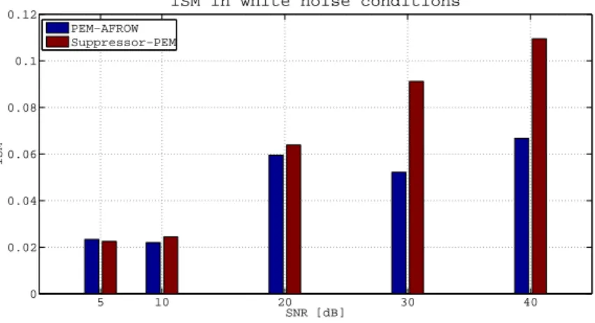
2.13 Log-Spectral Distortion in white noise conditions. . . 36

2.14 Itakura-Saito Measure in white noise conditions. . . 36

2.15 Overall Speech Reinforcement system block diagram. The f and r pedices stand for front and rear speaker position. . . . 38

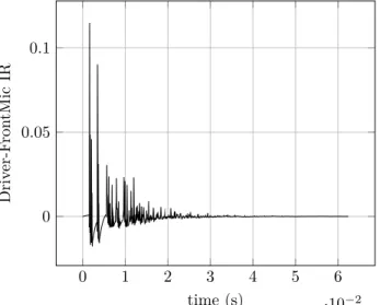
2.16 Impulse response between the front speaker and the front micro-phone. . . 43

2.17 Impulse response between the rear loudspeaker and the front microphone (feedback coupling). . . 44

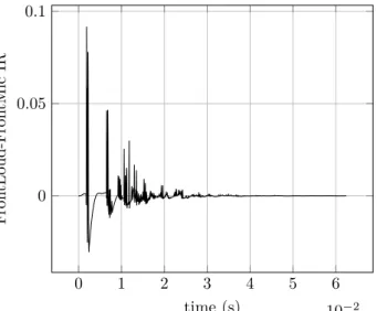
2.18 Impulse response between the front loudspeaker and the front microphone (echo coupling). . . 44

2.19 Channel 1 (a) and channel 2 (b) speech signals employed to simulate a double-talk-free scenario. . . 46

2.20 AFC misalignment in channel 1. . . 48

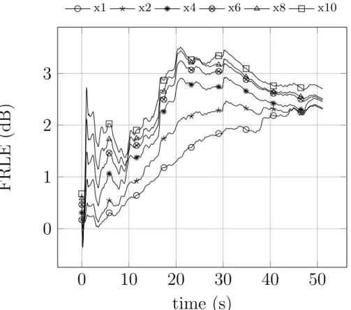
2.21 FRLE in channel 1. . . 49

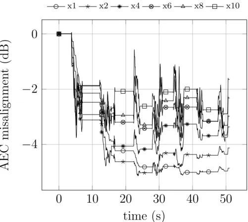
2.22 AEC misalignment in channel 1. . . 50

2.23 ERLE in channel 1. . . 50

2.24 Isolation in channel 1. . . 51

2.25 ISM in channel 1. . . 51

(18)

List of Figures

2.27 Channel 1 (a) and channel 2 (b) speech signals employed to

simulate a double-talk scenario. . . 55

2.28 AEC misalignment with 20% perturbed IR. . . 56

2.31 AFC misalignment with 20% perturbed IR. . . 58

2.34 AFC misalignment in channel 1. . . 60

2.35 FRLE in channel 1. . . 60

2.36 AEC misalignment in channel 1. . . 61

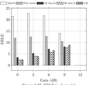
2.37 ERLE in channel 1. . . 61

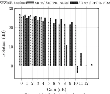
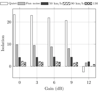
2.38 Isolation on channel 1. . . 62

2.39 ISM on channel 1. . . 62

2.40 LSD on channel 1. . . 63

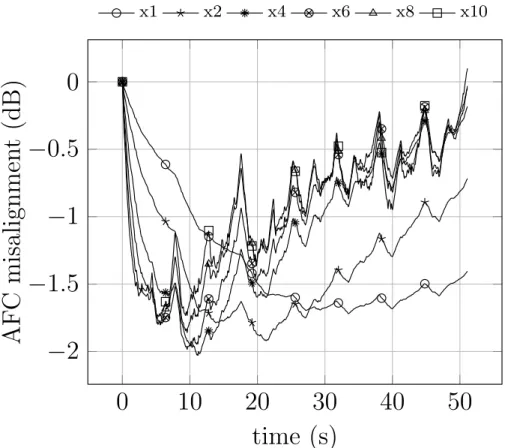
2.41 AFC misalignment in channel 1 by using different adaptive fil-tering stepsize values. . . 64

2.42 AEC misalignment in channel 1 by using different adaptive fil-tering stepsize values. . . 65

2.43 FRLE in channel 1 by using different adaptive filtering stepsize values. . . 66

2.44 ERLE in channel 1 by using different adaptive filtering stepsize values. . . 67

3.1 Standard LMS update scheme. Adaptive filter taps update is not consistent due to the presence of the secondary path transfer function S(z). . . . 73

3.2 FxLMS update scheme. Filtered version xf(n) of reference signal x(n) is needed to ensure adaptive filter taps update consistency. 74 3.3 Single tone NB-FxLMS block diagram. . . 74

3.4 Relation among disturbance tone amplitude A and ACNB-FxLMS taps w0 and w1. . . . 76

3.5 Single tone ACNB-FxLMS block diagram. . . 77

3.6 Error signal RMS level versus time for the classic NB-FxLMS algorithm in four different initial phase conditions. . . 79

3.7 Error signal RMS level versus time for the ACNB-FxLMS algo-rithm in four different initial phase conditions. . . 79

3.8 Error signals in instability condition cause by a lack of secondary path compesation. . . 80

(19)

List of Figures 3.9 Error signals using ACNB-FxLMS in five different case of

mis-takes on noise amplitude information. Mismis-takes are introduced equally on each harmonic order. . . 80 3.10 Generic ANC scheme. . . 82 3.11 Kalman filter configuration for wide-band single-channel systems. 83 3.12 Kalman filter configuration for a single-channel narrow-band

sys-tem. . . 84 3.13 Kalman filter configuration for wide-band multi-channel systems. 87 3.14 Kalman filter configuration for a multi-channel narrow-band

sys-tem. . . 89 3.15 Simulator speakers and microphones displacement considered in

single-channel systems simulations. . . 91 3.16 Simulator speakers and microphones displacement considered in

multi-channel systems simulations. . . 92 3.17 Wide-Band Single-Channel FxLMS Vs Kalman with pink noise. 93 3.18 Wide-Band Single-Channel FxLMS Vs Kalman with tonal noise. 93 3.19 Narrow-Band Single-Channel FxLMS Vs Kalman. . . 94 3.20 Wide-Band Multi-Channel FxLMS Vs Kalman with pink noise. 95 3.21 Wide-Band Multi-Channel FxLMS Vs Kalman with tonal noise. 96 3.22 Narrow-Band Multi-Channel FxLMS Vs Kalman. . . 96 3.23 Peugeot 407 SW, 2.0l, diesel. . . 97 3.24 Error microphones and anti-noise loudspeakers dislocation within

the cockpit. . . 98 3.25 Error signals on position 1 (driver) for multi-position algorithm. 100 3.26 Error signals on position 1 (driver) for single-position algorithm. 100 3.27 Error signals on position 2 (front passenger) for multi-position

algorithm. . . 101 3.28 Error signals on position 2 (front passenger) for single-position

algorithm. . . 101 3.29 Error signals on position 3 (rear central passenger) for

multi-position algorithm. . . 102 3.30 Error signals on position 3 (rear central passenger) for

multi-position algorithm. . . 102 3.31 Error signals on position 1 when with car marching on first gear. 103 3.32 Error signals on position 1 when with car marching on second

gear. . . 104 3.33 Error signals on position 1 when with car marching on third gear.105

(20)

(21)

List of Tables

2.1 Algorithm parameters . . . 43

2.2 Gain=3 dB, SNR=40 dB. . . 47

2.3 Gain=6 dB, SNR=40 dB. . . 47

2.4 Gain=10 dB, SNR=40 dB. . . 47

2.5 Average percentage of understood words (avg) in intelligibility tests and relative standard deviation (std). . . 49

2.6 Performance of the SR w/ SUPPR. NLMS algorithm in tests with different speech samples, Gain=6 dB, SNR=20 dB: average (avg) and standard deviation (std) values for quality indexes. . 53

2.7 Gain=6 dB, SNR=10 dB. . . 54

2.8 Gain=6 dB, SNR=20 dB. . . 54

2.9 Gain=3 dB, SNR=20 dB, Double-Talk. . . 54

2.10 Computational cost of the Speech Reinforcement system for the different implementations of the suppressor. . . 68

(22)

(23)

0.1 Introduction

The cabin of a marching vehicle is continuously permeated by noise and vi-brations, coming from the road, the wind and the engine itself. Audio and tactile feedbacks are continuously combined together, in a way and with an intensity strictly related to the specific environment, depending, for example, on the quality of cabin isolation, tires, windows, engine, fuel, number of peo-ple within the car and so on. These phenomena play an important role in the overall harmony of the vehicle and for this reason, driver and passengers could experience different situations from case to case, also depending on the model of the car and its brand. Possible sources for noise are manifold, and various approach to analyze and characterize them have been proposed in the literature [1]. Which component is predominant on other ones depends on speed, RPM, asphalt graininess and so no. In the following sections, from Sec-tion 0.1.1 to SecSec-tion 0.1.3 the main noise sources in automotive are described, while in Section 0.1.4 active approaches for enhancing comfort in automotive are introduced.

0.1.1 Engine and mechanical components

Cockpit isolation from engine noise has improved significantly over the years. However, some issues have not been resolved yet. Users often show adverse reactions when dealing with low frequency noises, especially if they are gen-erated by diesel engines. Unfortunately, as the wavelengths increase, classic passive isolation components get bulkier and not suitable, leaving costumers unsatisfied.

Another known issue is the so called "boom", occurring at a certain point while the engine is accelerating. It is caused by the engine transmitting excitation at its firing frequency to vehicle body panels, triggering acoustic resonances. Considering that sound quality perception is strongly related to noise charac-teristic changes, it appears clear that this could be perceived as a unwanted behavior. In fact, if engine loudness grows linearly with RPM, psycho-acoustic effect, for humans being, results quite enjoyable regardless of absolute SPL level; but if loudness exhibits a deviation of more than 6 dB with respect to the ideal linear trend, the focus on the noise unexpectedly increases, potentially annoying users. Same problem is presented by the noise which generates from driveline, usually consisting in few pure tones. The sound quality concern, in-deed, comes from the fact that noise level varies with RMP and time, drawing people attention.

(24)

List of Tables

0.1.2 Road Noise

As isolation from engine improves, road noise becomes increasingly more im-portant for overall sound quality within the cockpit. It comprehends two con-tributions:

• A broad-band air-rush type mainly occurring between 500 Hz and 1300 Hz. • A tonal type, typically around 200 Hz, caused by excitement of tire

acous-tic cavity modes.

Its intensity strongly depend, beside on speed, also on the asphalt graininess and tires quality as well. It usually starts to be noticeable at 40 km/h but its contribution on the overall noise is maximum between 60 km/h and 100 km/h. Beyond this range, wind noise becomes predominant.

0.1.3 Wind Noise

As said in Section 0.1.2, wind noise is predominant for speed above 100 km/h. It can comprehends contributions from different aerodynamic conditions:

• Noise due to the vehicle moving at high speed through the steady air, also related to vehicle shape and its cross-sectional area.

• Noise due to turbulence through slots around doors, hood, windshield, windows etc.

• Noise due to exterior varying wind conditions, such as cross-wind. • Beating noise due to cockpit Helmholtz resonance (around 10/20 Hz)

excited by the air flow when a rear window or the sunroof are partially open.

The typical wind noise spectrum is broad-band, with a heavy predominance of low frequencies, especially for steady wind noise, which has strong compo-nents in the range from 30 Hz to 65 Hz. A gusting noise, instead, due to its impulsiveness, has content over 300 Hz as well.

0.1.4 Active Comfort Enhancing Methods

In case of very rowdy environments, understanding speeches might became hard, especially within wide cockpits, where the distances among seats are sig-nificant. Communication difficulties are often experienced as uncomfortable situations by users, especially when facing long trips with other people. More-over, in industrial civilization, where the use of private cars is widespread, costumers are becoming more and more demanding and their expectation is to

(25)

0.1 Introduction have more and more comfortable cars as time goes by, pushing car manufac-tures to increasingly focus their efforts in innovative isolation systems. Passive approaches are usually cheap and effective against high frequency disturbances; nevertheless, when it comes to deal with low frequencies they become too bulky for suitable solutions. For these reason, active comfort-enhancing and speech-reinforcing methods have been extensively studied during last decades, and now that digital signal processors (DSP) are becoming powerful enough, practical applications are no longer prohibitive. These solutions are based on adaptive filters theory and attempt to predict disturbances which will be then deleted from the environment.

The thesis is organized as follow: in Chapter 1 classic adaptive filters ap-proaches in literature are described. Chapter 2 introduces acoustic feedback and echo cancellation for communication aids in cockpits, also proposing an innovative and effective approach. Chapter 3 deals with active noise control methods, explaining two different approaches from the literature, proposing a new algorithm and showing results of a practical application in a real car. Chapter 4 concludes the thesis making few final considerations on comfort en-hancing solutions described in previous chapters.

(26)

(27)

Chapter 1 Adaptive Filters for Comfort

Enhancement

Adaptive filters are already widely used to cope with a variety of issues where the knowledge of the environment features is the key of the solution. Exploiting this information it is possible, for example, to predict a desired signal not directly observable or separable otherwise. Several algorithms have been carried out during past decades, descending from gradient descent method or control theory.

Section 1.1 introduces the classic Least Mean Square (LMS) algorithm and some of its most common variants while Section 1.2 reports first the classic Kalman filter formulation and then its application to the IRs identification problem.

1.1 Least Mean Square

Least Mean Square (LMS) [2] is a linear adaptive filtering algorithm derived from steepest-descent. It belongs to the family of stochastic gradient algorithms and it was developed in 1960 by Widrow and Hoff. It consists in two basic processes:

1. A filtering process, which involves:

• A linear filter output computation in response to an input signal

x(n).

• An error estimate generation comparing the linear filter output to a desired signal d(n).

2. An adaptive process involving automatic filter parameters adjustment in accordance with the estimated error.

Its notoriety is due to its simplicity because it does not require neither mea-surements of pertinent correlation functions nor matrix inversions.

(28)

Chapter 1 Adaptive Filters for Comfort Enhancement

1.1.1 Classic LMS

LMS derives from steepest-descent approach. This latter is an iterative gradient-based algorithm which strictly follows negative gradient direction and update filter parameters as show by (1.1):

w(n + 1) = w(n) −µ

2∇J (n) (1.1)

where µ is the convergence factor, also known as step-size, and ∇J (n) is the error function gradient with respect w(n) given by (1.2).

∇J (n) = −2p + 2Rw(n) (1.2)

Correlation matrix R and cross-correlation vector p are respectively given by (1.3) and (1.4)

R = E[x(n)xT_(n)]

(1.3)

p = E [d(n)x(n)] (1.4)

However, in practice, prior knowledge of R and p is not available and the gradi-ent vector ∇J (n) must be estimated. The LMS goal is to exploit instantaneous estimate of R and p:

ˆ

R = x(n)xT(n) (1.5)

ˆ

p = d(n)x(n) (1.6)

Substituting (1.5) and (1.6) in (1.2) in place of R and p, gradient estimate is the following:

ˆ

∇J (n) = −2d(n)x(n) + 2x(n)xT_(n)w(n) _(1.7) From (1.1), filter parameters update formula for LMS algorithm becomes the following:

w(n + 1) = w(n) + µx(n)[d(n) − xT_w(n)]

(1.8) Here, xT_{w(n) is the adaptive filter output and d(n) − x}T_{w(n) is the error e(n).} Equation (1.8) could be, then, re-written in the following more familiar way:

w(n + 1) = w(n) + µx(n)e(n) (1.9)

At each iteration, LMS algorithm needs the most recent values of input signal

(29)

1.1 Least Mean Square

1.1.2 Variable Step-Size LMS

The step-size value µ in the LMS update equation (1.9) plays a fundamental role in determine the algorithm performances. Indeed, great step-sizes assure fast convergence rates but they also imply significant errors with respect opti-mal solution. On the contrary, sopti-mall step-sizes allow a more accurate solutions once the algorithm converged, but convergence rate results being strongly lim-ited. Therefore, a good trade-off has to be found when classic LMS approach is adopted, in order to have a sufficient convergence rate and an acceptable error. However, several approaches have been proposed in order to dynamically change step-size value while the LMS algorithm is running. The general idea is to in-crease it when the algorithm is still far from optimal solution and dein-crease it when a steady state is being reached. Several approaches have been proposed in the literature to achieve this goal.

One of the first proposed solutions is the so called heuristic strategy. It consists in monitoring the instantaneous gradient estimate ˆ∇J (n) and check how many consecutive sign inversions have occurred. If the sign changed M1 consecutive

times, the algorithm is close to convergence and the step-size value µ might be decreased of a predefined amount C1 in order to improve algorithm precision.

If the sign did not change in the last M2 steps, the algorithm is relatively far

from convergence and the step-size might be increased of a predefined amount

C2 to increase the convergence rate.

Another important solution is the Mathews’ approach [3], in which the step-size is updated in order to obtain a variation proportional to the gradient of squared error with respect to step-size µ itself, as show in (1.10).

µ(n) = µ(n−1)+ρ 2 ∂e2 n ∂µ(n − 1) = µ(n−1)+ρe(n)e(n−1) xT_{(n)x(n − 1)} ∥ x(n − 1) ∥2 (1.10)

where ρ is a positive constant used to control the step-size update, and ∥ · ∥2

is the Euclidean norm.

However, as reported in [4], whatever variable step-size method is adopted, convergence requirements during LMS adaptation limit the allowed step-size values, forcing the algorithm to use a bounded step-size ¯µ given by (1.11).

¯ µ(n) = ⎧ ⎪ ⎪ ⎨ ⎪ ⎪ ⎩ µmax if µ(n) > µmax µmin if µ(n) < µmin µ(n) otherwise (1.11)

In this way, instability situations due to excessive large step-sizes are avoided, as well as unresponsive ones due to excessively small values.

(30)

Chapter 1 Adaptive Filters for Comfort Enhancement

1.1.3 Normalized LMS

An alternative to variable step-size LMS described in Section 1.1.2 is the Nor-malized LMS (NLMS). This is a variant of classic LMS that attempts to de-crease algorithm sensitiveness to the amplitude scaling of input signal x(n). The basic idea is to divide step-size value µ by the power of input signal x(n), in order to obtain smaller step-sizes when this latter is strong and greater ones when it is weak, according to the following equation:

µ = µ

′

c + xT_(n)x(n) (1.12)

where µ′_{is a basic constant step-size and c is an arbitrary small constant}

intro-duced to avoid division by 0 or excessively small values when x(n) approaches zero. NLMS algorithm is very effective when strong changes in the input sig-nal x(n) power occur, as it might happen, for example, in the case of speech signals.

1.1.4 Leaky LMS

Leakage LMS is obtained introducing in classic LMS update equation (1.9) a "leakage" factor γ, also known as "forgetting" factor. The update equation is the following:

w(n + 1) = γw(n) + µx(n)e(n) with 0 < γ < 1 (1.13) In this way, the effect of sample x(n) at a given time step, decreases while temporal index increases. Leakage LMS might be useful in several practical applications where there are localized errors in input signal x(n).

1.1.5 Sign LMS

In some practical applications, classic LMS computation burden might result too high to be handled with available hardware. In such cases, an approxima-tion of classic LMS update equaapproxima-tion (1.9) could be useful. Possible soluapproxima-tions are the following:

1. Sign Algorithm:

w(n + 1) = w(n) + µsign(e(n))x(n) (1.14)

2. Clipped LMS:

(31)

1.1 Least Mean Square 3. Sign-Sign:

w(n + 1) = w(n) + µsign(e(n))sign(x(n)) (1.16)

In above equations, operator "sign" denotes the sign operation reported below:

sign(z) = ⎧ ⎪ ⎪ ⎨ ⎪ ⎪ ⎩ 1 if z > 0 0 if z = 0 −1 if z < 0 (1.17)

First two solutions allow to reduce the number of multiplications, while last one completely avoids them. However, algorithm robustness decreases because the greater the approximation, the more troublesome the algorithm convergence becomes.

1.1.6 Smoothing LMS

The smoothing LMS algorithm is used when the gradient estimate e(n)x(n) is noisy. Depending on what kind of smoothing is applied, there are several version of this solution.

One of the most famous is the Averaged LMS, where the gradient estimate is substituted with its average on N samples. The update equation formula is the following: w(n + 1) = w(n) + µg(n) (1.18) where g(n) is given by (1.19). g(n) = 1 N n ∑ j=n−N +1 e(j)x(j) (1.19)

As shown by equation (1.20), the kthcomponent of g(n) might be also seen as a convolution with a rectangular window, whose impulse response h(n) is given by (1.21) gk(n) = 1 N n ∑ j=n−N +1 e(j)x(j − k) = h(n) ∗ {e(n)x(n − k)} (1.20) h(n) =[ 1 N, 1 N, · · · , 1 N ] (1.21) Since a rectangular window is substantially a low pass filter, the gradient av-erage g(n) can be generically expressed as follows:

(32)

Chapter 1 Adaptive Filters for Comfort Enhancement with h(n) an impulse response of a generic low pass filter.

Another solution for smoothing LMS is the so called Momentum LMS. It use a simple first order FIR to obtain a gradient estimate given by equation (1.23).

g(n) = (1 − γ)g(n − 1) + γ {e(n)x(n)} with 0 < γ < 1 (1.23) The gradient is practically filtered with the following response:

G(z) = γ

1 − (1 − γ)z−1 (1.24)

Since we have:

w(n + 1) − w(n) = µg(n) (1.25)

exploiting equation (1.23) and (1.25), the Momentum LMS updating formula is the following:

w(n + 1) = w(n) + µg(n) =

= w(n) + (1 − γ)(w(n) − w(n − 1) + µγe(n)x(n) = w(n) + µ′e(n)x(n) + α (w(n) − w(n − 1))

(1.26)

where µ′= µγ and α = (1−γ). Term α (w(n) − w(n − 1)) is called momentum

term, while remaining one is the usual LMS contribution.

These approaches’ goal is to improve performances at a steady state, but ob-viously this could affect convergence rate.

1.2 Kalman Filter

Kalman filter refers to an efficient recursive algorithm used in adaptive filters, named after its primary developer, Rudolf Emil Kálmán. This algorithms orig-inates from a generic system identification problem [5] and it is able to obtain an estimate of system state variables exploiting system inputs/outputs mea-surements, even if affected by some kind of noises and inaccuracies. In this section the classic Kalman filter theory for discrete time applications is briefly described. Section 1.2.1 describes the model to which a system should fit in order to be able to exploit the Kalman filter theory. Section 1.2.2 explains how the updating process works.

1.2.1 Kalman Filter Model

In order to use the Kalman filter properly, it is important to make sure that the problem to be solved fits its conditions. Kalman filter aims find an estimate ˆ

(33)

1.2 Kalman Filter the linear stochastic difference equation (1.27), such that the estimated output ˆ

yk = Hkxˆk is as close as possible to the ideal output yk = Hkxk. This is achieved exploiting a measurement zk ∈ ℜmof yk, given by (1.28).

xk = Akxk−1+ Bkuk+ wk−1 (1.27)

zk = yk+ vk= Hkxk+ vk (1.28) The subscript k represents the discrete time interval. Process noise and mea-surement inaccuracy are represented by the random variables wk and vk re-spectively. n × n matrix Ak represents the relation between the current state

xk and the previous one xk−1. n × l matrix Bk represents the relation between the (optional) control inputs uk ∈ ℜl and the current state xk. m × n matrix

Hk represents the relation between the current state xkand the current output

yk. The measure zk is an observation of the system output yk itself.

If the system to be controlled can be modeled by previous equations, then a Kalman filter solution can be applied. Matrices Ak, Bk and Hk elements may potentially change at each time step k, but here only matrix Hkwill be assumed time-varying.

1.2.2 Updating Process

Kalman filter exploits two distinct updates to achieve its goal: a prediction update, which projects forward in time the current state and error covariance estimates, and a correction update, which represents a feedback for the system, correcting the previous estimates through the knowledge of measure zk. The time update consists in the following two equations:

1. State prediction.

ˆ

x−_k = Aˆxk−1+ Buk (1.29)

2. Error covariance prediction.

P_k−= APk−1AT + Q (1.30)

ˆ

x−_k and P_k−represent the prior estimates of the state xkand the error covariance

Pk respectively, i.e. the estimates before the measurement update correction. In (1.30), Q represents the process noise covariance and its values is meant to be tuned in most case empirically.

(34)

Chapter 1 Adaptive Filters for Comfort Enhancement 1. Kalman gain computation.

Kk =

P_k−HT k

HkPk−HkT + R

(1.31)

2. State estimate update via measurement zk. ˆ

xk = x−k + Kk(zk− Hkxˆ−k) (1.32)

3. Error covariance estimate update. ˆ

Pk= (I − KkHk)Pk− (1.33)

In (1.31), R represents the measure noise covariance and, unlike the process noise covariance Q, is relatively simple to determine because it refers to the noise in the environment. Equation (1.32) compute an a posteriori estimate of the state xk as a linear combination between its a priori estimate x−k and a weighted difference (called residual or innovation) between an actual noisy measure zk and a measure’s prediction Hkxˆ−_k. If these two are equal, the a

pri-ori state estimate ˆx−_k do not need any correction; otherwise, if they mismatch, ˆ

x−_k is modified. As shown in Fig. 1.1, the only signals that the update process need from the outer system are the the input matrix Hk and the measurement

zk. The algorithm proceeds iterating between the time update and the correc-tion update at each time step, using prior values given by (1.29) and (1.30) to obtain the final estimates given by (1.31), (1.32) and (1.33). Kalman gain K is

xk Kalman vk Hk ˆ xk wk uk zk yk ˆ yk

Figure 1.1: Classic Kalman filter update scheme.

an n × m matrix and the way it is computed ensure that the a posteriori error covariance Pk is minimized. Mathematically, (1.31) is achievable following the

(35)

1.2 Kalman Filter steps reported below:

• Consider the a posteriori error equation (1.34) representing the mismatch between the actual state and a posteriori state ˆxk given by (1.32).

ϵk= xk− ˆxk (1.34)

• Substitute equation (1.32) in definition (1.34) and then the result in a

posteriori error covariance equation (1.35).

Pk = E[ϵkϵkT] (1.35)

• Derive the resulting equation with respect the Kalman gain K. • Set the result equal to zero and solve for Kalman gain K.

From (1.31) we can observe that as the measurement error covariance R ap-proaches zero, the Kalman gain K increases, giving more importance to the innovation (zk− Hkxˆ−k) in (1.32). This can also be interpreted as an increasing trust on measure zk as R decreases. On the other hand, if the a priori error covariance P_k− given by (1.30) decrease, Kalman gain decrease as well, which means that the measurement zkis less important for the final state estimation.

1.2.3 Kalman Filter for IRs Identification

It is easy to fit an Impulse Response (IR) identification problem into Kalman filter theory, as shown in Fig. 1.2. Representing the IR as a Finite Impulse

xk Kalman Hk ˆ xk -wk ek vk zk yk

Figure 1.2: Kalman filter configuration for IR identification.

(36)

Chapter 1 Adaptive Filters for Comfort Enhancement aims to estimate is represented by the FIR’s taps themselves.

xk = ⎛ ⎜ ⎜ ⎜ ⎜ ⎝ xk,1 xk,2 .. . xk,n ⎞ ⎟ ⎟ ⎟ ⎟ ⎠ (1.36)

The signals yk and zk, instead, are the system output and its measurement respectively. Following this hints, matrix Hk, which as said before represents the relation between the current state xk and the current output yk, inevitably contains the system input signal rk, often referred to as reference. Equation (1.37) clarifies how Hk is composed.

Hk= (

rk rk−1 · · · rk−n+1 )

(1.37) Control input signals uk are actually optional, since in many practical appli-cations, such as ANC systems, they are not present at all because there is no way of governing the overall environment behavior.

(37)

Chapter 2 Communicational Comfort

Enhancemen Through Acoustic

Feedback and Echo Cancellation

Communicational comfort might be compromised in some cases because of the noise and/or distances among seats. Hearing aids are often used in order to assist conversations, but any time an audio signal is acquired by a microphone and reproduced (once elaborated) by means of a loudspeaker within the same room environment, an acoustic coupling between the two devices arises. This means that an acoustic feedback may occur and seriously deteriorate the audio rendering performance of the overall system and limit the maximum channel gain attainable, typically expressed as maximum stable gain (MSG). Speech reinforcement techniques aim to improve the speech quality in presence of ad-verse acoustic conditions in order to produce a comfortable communication experience.

According to the Nyquist Stability Criterion [6, 7], a closed-loop system is unstable if there exist a harmonic pulse ω = 2π(_ff

s )

in correspondence of which the following conditions hold:

{

G (ω, t) F (ω, t) ≥ 1,

∠G (ω, t) F (ω, t) = n2π, n ∈ Z (2.1)

where G (ω, t) is the forward path transfer function and F (ω, t) the acoustic feedback path transfer function. The acoustic instability is typically exhibited as a howling (also known as Larsen effect).

Different techniques have been proposed in the literature to solve the prob-lem [8, 9, 10]. A widely used and robust approach, belonging to the category of

gain reduction methods, exploits notch-filter-based howling suppression (NHS)

techniques. They recover from an instability situation by reducing the gain in correspondence of those frequencies where howling occurs. The cons is that, in the first place, the howling must appear in order to be detected and suppressed.

(38)

Chapter 2 Communicational Comfort Enhancemen Through Acoustic Feedback and Echo Cancellation Typically, the NHS algorithms are able to detect the feedback occurrence with

a significant processing latency, which acceptability in a communication sce-nario is questionable.

In order to suitably face the issue, solutions based on the acoustic feedback path estimate called room modeling methods, have been recently developed. These allows to obtain an estimate of the system feedback component which is then suitably subtracted from the acquired microphone signal. The better the estimate, the deeper the feedback cancellation will be and therefore the higher the MSG will result. Acoustic feedback cancellation (AFC) approach is based on this solution. Conceptually, the problem addressed is similar to the acoustic echo cancellation AEC one [11, 12], but with the substantial difference that the source signal in the AFC scheme is highly correlated with the signal coming from the loudspeaker (since the speaker source acts in the same acoustic envi-ronment), which results in a biased estimation process.

To overcome this problem, in [9, 13] an interesting technique based on the Prediction Error Method (PEM ) is proposed. This solution, named Predic-tion Error Method based on Adaptive Filtering with ROW operaPredic-tions (PEM-AFROW), consists in decorrelating signals by means of time-varying whiten-ing filters and then uswhiten-ing them for the main adaptive estimation process. The main advantage is that decorrelation process does not influence the microphone signal characteristics since it takes place within the adaptive filtering circuit. In [14] the previous approach has been further improved by means of a suppres-sor filter. It has been shown that the introduction of this latter can increase the performances in terms of robustness and stability, leading to an overall approach named Suppressor-PEM. This solution can be extended to deal with a dual-channel scenario to support a bidirectional communication. The man-agement of two channels increases the algorithm complexity since, besides the feedback effects, echoes between channels occur as well. However, in this way the system becomes more suitable for real applications, allowing the two speak-ers to communicate. This idea has been previously explored in [15] and is hereby described in a more comprehensive way.

Some interesting dual-channel communication based solutions have been re-cently proposed in the literature. In [16] Ortega suggests an approach where only the echo effects are taken into account and additional echo suppressor fil-ters are used to compensate the lack of AFC filfil-ters. Furthermore, in [17] and in [18], Schmidt develops an AFC system making use of a loss control unit which reduces the channel gains in the absence of speech and using decorrelation methods working in the closed signal loop, introducing unavoidable collateral distortion.

This chapter is organized as follows. In Section 2.1 the PEM-AFROW al-gorithm and its frequency implementation are described. Section 2.2 describes

(39)

2.1 The PEM-AFROW Algorithm how a suppressor filter works and the two alternative implementations sug-gested. In Section 2.3 a hybrid an HW/SW test-bench is proposed while Sec-tion 2.4 analyzes some experimental results obtained with aforemenSec-tioned test-bench. Dual-channel issues are faced in Section 2.5 and Section 2.6 shows some simulations of dual-channels scenarios analyzing related results.

2.1 The PEM-AFROW Algorithm

The architecture of the PEM-AFROW algorithm acting on a single-channel feedback cancellation scenario is reported in Fig. 2.1 along with the notation used hereafter. In analogy to Eq. (2.1), the term F (q) denotes the acoustic feedback path from the loudspeaker to the microphone, s(t) and d(t) the clean speech signal and the background noise respectively.

Inspired by the notation used in [19], q−1 denotes the unitary delay, so that

q−1u(t) = u(t − 1) and it is possible to represent a discrete time filter with

finite length L as a polynomial in q:

F (q) = f0+ f1q−1+ · · · + fL−1q−L+1= fTq. (2.2) The filtering operation consists in applying the polynomial to the input se-quence (F (q)u(t) = fT_{u(t), u(t) = (u(t), u(t − 1), · · · , u(t − L + 1))}T_{). The} feedback canceller ˆF (q) estimates the feedback signal v(t) (that is the result

of filtering the loudspeaker signal u(t) with the filter F (q)) and subtracts it from the microphone signal y(t) before being amplified by a gain factor K and played back by the loudspeaker. The block z−∆ in Fig. 2.1 models the delay always present in a real system implementation (due to A/D and D/A conver-sions, processing and propagation delays), that also guarantees the loudspeaker-enclosure-microphone (LEM) path identifiability, as stressed later on.

Classical direct identification techniques, like the ones used in AEC algo-rithms, cannot be employed to identify unknown acoustic path F (q) in closed loop configuration. Indeed the basic assumption made in a typical AEC frame-work is that the near end signal s(t) is uncorrelated with the loudspeaker signal

u(t), so that the acoustic path can be estimated during the echo-only period

(absence of near end signal). On the contrary, in AFC problem, due to the feedback, the two signals are inevitably correlated and a direct identification of the acoustic path (i.e. performed as if the system operates in open loop) would lead to a biased feedback path estimate ˆF (q).

Feedback path estimate is formally equivalent to a problem known in the lit-erature as closed-loop system identification (CLI) [20], for which a class of solutions based on the prediction error method (PEM) can be applied, leading, under certain conditions, to an unbiased estimate of the feedback path. An

(40)

in-Chapter 2 Communicational Comfort Enhancemen Through Acoustic Feedback and Echo Cancellation ˆ F (q) F (q) u(t) e(t) ˆ v(t) v(t) d(t) s(t) w(t) System to be indentified

Acoustic feedback path

H(q) y(t) Z−∆ Σ − K G(q)

Figure 2.1: Acoustic feedback cancellation.

teresting implementation of this concept is the aforementioned PEM-AFROW algorithm. As for any PEM-based AFC algorithm, the basic assumption of the PEM-AFROW is that the near end signal, can be modeled by the expression

H(q)w(t), where w(t) is white noise and H(q) is known and inversely stable, so

that the inverse filter of H(q) (say A(q) = H−1(q)) can be used to decorrelate the signals in the identification task. However, H(q) is not only unknown but also time-varying, therefore it has to be estimated in an adaptive way together with F (q). In [19] it is proved that if H(q) is a P -order AR process, the iden-tification of H(q) and F (q) can be done simultaneously, assuming the presence of a forward delay ∆ bigger than the H(q) filter order. PEM, applied to the system in Fig. 2.1, leads to the following cost function:

Jp= 1 N N −1 ∑ k=0 e2_p(t), ep(t) = ˆA (q) [ y (t) − ˆF (q) u (t)], (2.3)

Equation (2.3) that must be minimized to get the optimal values for { ˆA(q), ˆF (q)}.

Note that (2.3) is nonlinear in { ˆA(q), ˆF (q)}. Modelling the near end signal by a

time varying AR (TVAR) model of order P , introducing a delay ∆ > P in the forward path and supposing than the TVAR model is stationary over frames of 20 ms, the estimations of A(q) (the inverse of the near end signal AR model) and F (q) in (2.3), can be decoupled in two disjoint steps, on a frame by frame basis, as described below.

(41)

2.1 The PEM-AFROW Algorithm time-varying AR (TVAR) model over a Lf samples frame, as follows:

s (t) = a1s (t − 1) + · · · + aPs (t − P ) + w (t) , (2.4) where w(t) is a white noise excitation sequence. Since the feedback path is usually stationary over intervals longer than the assumed speech station-ary period, we would need an approach which allows to estimate the AR model and the LEM path over frames of different length, by minimizing the cost function (2.3). Therefore, assuming the stationarity of the AR model

a(t) = (1, −a1(t), · · · , −aP(t))T = ˆai, with l = ⌈k/Lf⌉ over a speech frame, the PEM-AFROW is able to decouple the estimation of ˆai and ˆf (t) in two disjoint steps, on a frame by frame basis.

In the first step, the ˆf (lLf− 1) estimate, obtained in the previous frame pro-cessing, is used to filter the loudspeaker signal (t = lLf, · · · , (l + 1)Lf− 1), and the result is subtracted from the correspondent values of y(t), giving

e(t) = y(t) − uT(t)ˆf (tLf− 1). (2.5)

The Levison-Durbin algorithm is then applied to the Lf frame sample values of

e(t) to find the linear prediction error filter ˆai for frame l. In the second step, the ˆalestimate (constant over that frame) is used and the PEM minimization problem to be solved coincides with a generic adaptive filtering problem to be applied to whitened signals. The input vector to the adaptive filtering algorithm is ˜ uT(t) = aT_l ⎛ ⎜ ⎜ ⎝ uT_(t) .. . uT_{(t − P )} ⎞ ⎟ ⎟ ⎠ , (2.6)

and the desired signal aT_l (y (t) , · · · , y (t − P ))T. Since ˆal is constant over the frame of interest, a single vector multiplication has to be performed at each iteration, and only once per frame, after the ˆal update, the complete vectors has to be recomputed, demanding a matrix multiplication. This makes the algorithm computationally advantageous. It must be noted that in the voiced speech case the w(t) is periodic and, in order to achieve a better decorrelation, it would be preferable to implement a Long Term Prediction to model such a periodicity, in cascade to the first predictor, as effectively done in [13]. It is possible to repeat the previous two steps in an iterative way to improve the convergence; nevertheless, to keep the computational load low, one single iteration has been adopted.

The main advantage of PEM-AFROW is its pro-activity, that is the ability to cancel feedback before the howling becomes perceivable. Moreover, thanks to its remarkable identification ability, once a stable condition is achieved, it can

(42)

Chapter 2 Communicational Comfort Enhancemen Through Acoustic Feedback and Echo Cancellation effectively cancel the feedback without introducing a collateral distortion in the

speech signals.

To provide a real-time application for this approach, the PB-FDAF algorithm [2, 21] has been taken into consideration for the identification issue of f (t). The reasons for this choice reside in the number of advantages that this algorithm provides, i.e., fast convergence, low computational complexity and low process-ing latency, as confirmed by experimental results discussed in the conclusive sections.

2.1.1 Frequency-Domain Algorithm Implementation

As previously stated, a frequency-domain adaptation can lead to several advan-tages, including a frequency-varying step-size and a fast convergence. However, in order to work in real-time and minimize the process delay, a decrease of com-putational complexity is needed. This is achieved by the PB-FDAF algorithm which considers the impulse response to estimate as divided into M different partitions.

Let N be the total number of weights to be modeled and M be the number of blocks, so that the N -taps feedback canceler ˆf (t) can be partitioned into M segments of length R = N/M each, which are then transformed to the

fre-quency domain by means of a NDF T points DFT (efficiently implemented as an FFT), with NDF T equal to the smallest power of two larger than or equal to 2R. PB-FDAF algorithm works on a M blocks queue of overlapped data and a Lf-dimensional frame of new input samples is processed at each itera-tion. The first step requires shifting the earlier block input vectors one position ahead into the queue, discarding the last block, while the incoming samples are converted to the frequency domain and stored on top of the queue:

Um(l) = diag ⎧ ⎪ ⎪ ⎨ ⎪ ⎪ ⎩ F ⎛ ⎜ ⎜ ⎝ u((l + 1)Lf− mR − NDF T + 1) .. . u((l + 1)Lf− mR) ⎞ ⎟ ⎟ ⎠ ⎫ ⎪ ⎪ ⎬ ⎪ ⎪ ⎭ , (2.7)

where m = 0, · · · , M − 1 and F is the NDF T × NDF T DFT matrix. The parameter 2Lfis the block length, which corresponds to an input/output delay of 2Lf − 1. Since, to transform the input vector, only one DFT per block iteration is needed, a significant saving in computation can be obtained.

(43)

2.2 The SUPPRESSOR-PEM Algorithm The output and error vectors can be expressed as:

zl= [ 0 ILf ]F −1 M −1 ∑ m=0 Um(l) ˆFm(l) , (2.8) el= yl− zl, (2.9) yl= [ y(lLf + 1) · · · y((l + 1)Lf) ] , (2.10) E (l) = F [ 0M −Lf el ] . (2.11)

The weight update equation is given by: ˆ Fm(l + 1) = ˆFm(l) + Γ (l) F gF−1UHm(l) E (l) , (2.12) where g = [ IR 0 0 INDF T−R ] . (2.13)

Γ (l) is a diagonal matrix which entries are the stepsize values µk(l), where k is the frequency bin. The stepsizes are normalized according to the sum of the input power Pu,k(l) and the error power Pe,k(l):

µk(l) = µ_k β + Pu,k(l) + Pe,k(l) , k = 0, . . . , N′− 1, (2.14) with Pu,k(l) =∑M −1_m=0∥Um,k(l) ∥2, Pe,k(l) = R∥Ek(l) ∥2, (2.15)

∥ · ∥2 _{being the squared norm operator, i.e., ∥x∥}2 ₌ ∑ i,jx

2

i,j. This normal-ization of the step size with the sum of the input and error power reduces the excess error in the presence of desired signals with large power fluctuations and signal onsets. The term β is a small constant added to avoid divergence problems in silence periods.

In the current implementation, PB-FDAF algorithm has been implemented with partition length R = Lf.

2.2 The SUPPRESSOR-PEM Algorithm

The PEM-AFROW algorithm, especially when in stable conditions, showed to have good feedback cancellation performance without introducing distortion. Nevertheless, it is pointed out in [22] and [23] that the tracking behavior of the

(44)

Chapter 2 Communicational Comfort Enhancemen Through Acoustic Feedback and Echo Cancellation PEM-AFROW is non-perfect, which may lead to an unstable system, especially

when operating close to the stability threshold. In particular, changes in the acoustic feedback path (due, for example, to moving objects and/or abrupt increasing loop gain) have shown to be quite troublesome from this perspective. In presence of a dual-channel communication, such a sensitivity is relevantly stressed, as a consequence of occurrence of multiple acoustic couplings and of simultaneous adaptation of feedback and echo cancelers operating in Speech Reinforcement system.

A new approach, named Suppressor-PEM, employing a feedback suppression filter in cascade with the PEM-AFROW algorithm, as shown in Fig. 2.2, has been recently presented in [15]. It has been experimentally proved that such a solution is more robust with respect to the single PEM-AFROW algorithm. By varying the α parameter, the feedback suppressor filter switches from a pre-diction error filter (PEF) (α = 1) to an infinite impulse response (IIR) adaptive oscillator (α = 0). In PEF mode, the filter attenuates those frequencies which violates the Nyquist stability criterion, as long as any integer multiple of the inverse of the howling frequency is larger than ND and smaller than ND+ NC samples, where NC is the filter length and ND is a convenient delay. On the other hand, when configured as IIR adaptive oscillator, it allows to achieve very narrow notches [17]. The NDsamples delay, usually set to 2 ms, is necessary to introduce a de-correlation in the signals, in order to avoid speech cancellation. When operating in a PEF configuration, due to the periodic or quasi-periodic nature of speech signal, the finite impulse response (FIR) filter length should not exceed 80-120 coefficients (at 16 kHz sampling rate), which roughly corre-sponds to a pitch period. The choice of the adaptive filtering step-size is of crucial importance, trading off between accuracy and fast convergence. Indeed, while a small value avoids speech signal suppression, a larger value guarantees faster convergence.

Since the suppressor filter length is shorter than the other adaptive filter length (i.e., the AFC filter), a time-domain based implementation for the sup-pressor does not exasperate too much the computational complexity of the whole system. For this reason, two algorithms have been considered for adap-tive filtering in the suppressor case study: the Normalized Least Mean Squares (NLMS ) and the frequency domain adaptive filtering (FDAF ) [2].

2.2.1 Suppressor NLMS

Adaptive filtering algorithm adopted by this version is the NLMS algorithm, which operates in the time domain. In systems where the other filters work in the frequency domain (like those developed in this work) and one frame of D samples at a time is taken into account, an additional loop to consider

(45)

2.2 The SUPPRESSOR-PEM Algorithm ˆ F (q) F (q) u(t) e(t) ˆ v(t) v(t) Z−ND K PEM-AFROW Σ − Σ e′(t) × × + (1 − α) α ˆ n(t) c(t) ˜ e(t) Z−∆ Suppressor

Figure 2.2: SUPPRESSOR-PEM algorithm block scheme.

one sample at a time is needed to apply this kind of suppressor filter. The behaviour of this approach within this loop is described hereafter. The signal

s(t) is first processed by the PEM-AFROW algorithm and the related output

by the suppressor filter. The suppressor first computes the signal ˜e(t) as follows:

˜

e(t) = α · e(t) + (1 − α) · ˆn(t), (2.16)

Subsequently the signal ˆn(t) is computed applying the ND samples delay to a buffer ˜e(t) and filtering it through the suppressor filter c(t):

ˆ

n(t) = c(t)T˜e(t − ND). (2.17)

ˆ

n(t), representing the residual feedback, is then subtracted from the signal e(t)

to obtain e′(t), which will be finally amplified and sent to the loudspeaker. The update equation for the suppressor filter using the NLMS algorithm is the following:

c(t + 1) = c(t) + µc(t)˜e(t)e′(t), (2.18) with

(46)

Chapter 2 Communicational Comfort Enhancemen Through Acoustic Feedback and Echo Cancellation and µc(t) = ˜ µc β + σ2 c(t) , (2.20)

where µc(t) is the time-varying step-size, ˜µc is a proper control parameter,

σ2

c represents the variance of ˜e(t) and β is a proper positive number which avoids divisions by either zero or too small values when σc2(t) decreases. This implementation of the Speech Reinforcement system is named SR w/ SUPPR.

NLMS.

2.2.2 Suppressor FDAF

In this Suppressor version, adaptive filtering algorithm works in the frequency domain. Therefore, since it already considers a frame of Lf samples at a time, it does not need additional loops. The adopted algorithm is the FDAF (Fre-quency Domain Adaptive Filtering) which is substantially the same used by the AFC filters but with a single partition because of the shorter size of the suppressor filter length Nc. Indeed, it would be useful to set this latter equal to the length of an AFC filter single partition.

Just like in the time domain, the input signal is first processed by the PEM-AFROW algorithm for feedback cancellation and the AFC filter update. Af-terwards a new frame l of the signal ˜e(t) (suppressor filter input) is computed:

˜

e(l) = α · e(l) + (1 − α) · ˆn(l). (2.21) Then, this is converted in frequency domain by an FFT using a number of points twice the number of samples in the time domain. To accomplish this, zero-padding in the frame queue is not recommended, since rustling may emerge in the loudspeaker signal. The adopted solution consists in keeping two previous frames in the system memory (using buffers) and properly concatenate them together with the current one to obtain a double sized frame. Two previous frames are needed, instead of just one, because last ND samples of the current frame ˜e(l) have to be discarded, due to the NDsamples delay to be introduced. Therefore, the samples of the previous frame ˜e(l − 1) are not enough to obtain

a double sized frame, and ND samples of the even previous one ˜e(l − 2) are needed (Fig. 2.3). Following the formalism of Section 2.1.1 and bearing in mind that in this case there is no partitioning (M = 1), the DFT of ˜e(t) is

(47)

2.2 The SUPPRESSOR-PEM Algorithm

Current frame Last frame

Second-to-last frame

Double-sized frame to be transformed

ND samples delay ND samples delay

Figure 2.3: Frame concatenation before the FFT computation.

˜

E(l) = F (˜e(t)). The output and error vectors can be expressed as: ˆ nl= F−1E (l) ˆ˜ C (l) , (2.22) e′l= el− ˆnl, (2.23) el= [ e(lLf+ 1) · · · e((l + 1)Lf) ] , (2.24) E′(l) = F e′l. (2.25)

The weight update equation is given by:

C (l + 1) = C (l) + Γ (l) F gF−1E (l) E˜ ′(l) . (2.26)

For each frequency bin k the step size µk(l) is normalized according to the sum of the input power PE˜(l) and the error power PE′_,(l):

µk(l) = µ_k β + P_E˜(l) + PE′_,(l) , (2.27) with P_E˜(l) = ∥ ˜El(l) ∥2, PE′(l) = ∥E′_k(l) ∥2. (2.28)

The term β is a small constant added to avoid divergence problems in silence periods. This implementation is named SR w/ SUPPR. FDAF. With respect to the SR w/ SUPPR. NLMS, the SR w/ SUPPR. FDAF yields to a less accurate estimate since the FDAF algorithm is equivalent to a Block-NLMS algorithm, leading to a slightly lower effectiveness. However, the positive counterpart is a lower computational complexity leading to a faster execution, which is a primary feature for real-time applications.