A POLITICAL ECONOMY MODEL OF THE VERTICAL FISCAL GAP AND VERTICAL
FISCAL IMBALANCES IN A FEDERATION
Bev Dahlby, Jonathan Rodden
Document de treball de l’IEB
2013/18
Documents de Treball de l’IEB 2013/18
A POLITICAL ECONOMY MODEL OF THE VERTICAL FISCAL GAP AND VERTICAL FISCAL IMBALANCES IN A FEDERATION
Bev Dahlby, Jonathan Rodden
The IEB research program in Fiscal Federalism aims at promoting research in the public finance issues that arise in decentralized countries. Special emphasis is put on applied research and on work that tries to shed light on policy-design issues. Research that is particularly policy-relevant from a Spanish perspective is given special consideration. Disseminating research findings to a broader audience is also an aim of the program. The program enjoys the support from the Foundation and the
IEB-UB Chair in Fiscal Federalism funded by Fundación ICO, Instituto de Estudios Fiscales
and Institut d’Estudis Autonòmics.
The Barcelona Institute of Economics (IEB) is a research centre at the University of Barcelona which specializes in the field of applied economics. Through the
IEB-Foundation, several private institutions (Applus, Abertis, Ajuntament de Barcelona,
Diputació de Barcelona, Gas Natural and La Caixa) support several research programs.
Postal Address:
Institut d’Economia de Barcelona Facultat d’Economia i Empresa Universitat de Barcelona
C/ Tinent Coronel Valenzuela, 1-11 (08034) Barcelona, Spain
Tel.: + 34 93 403 46 46 Fax: + 34 93 403 98 32
http://www.ieb.ub.edu
The IEB working papers represent ongoing research that is circulated to encourage discussion and has not undergone a peer review process. Any opinions expressed here are those of the author(s) and not those of IEB.
Documents de Treball de l’IEB 2013/18
A POLITICAL ECONOMY MODEL OF THE VERTICAL FISCAL GAP AND VERTICAL FISCAL IMBALANCES IN A FEDERATION
Bev Dahlby, Jonathan Rodden
ABSTRACT: We develop a political economy model of intergovernmental transfers. Vertical fiscal balance occurs in a federation when the ratio of the marginal benefit of the public services provided by the federal and provincial governments is equal to their relative marginal costs of production. With majority voting in national elections, the residents of a "pivotal province" will determine the level of transfers such that the residents of that province achieve a vertical fiscal balance in spending by the two levels of government. We test the predictions of the model using Canadian time series data and cross-section data for nine federations.
JEL Codes: H71, H73, H77
Keywords: Fiscal federalism, vertical fiscal imbalance, fiscal gap
Bev Dahlby
School of Public Policy and Department of Economics
University of Calgary 5th Floor 906 8th Avenue
SW, Calgary Alberta, T2P 1H9 Canada Email: [email protected]
Jonathan Rodden
Department of Political Science Stanford University
616 Serra Street, Encina Hall Central, Room 444
Stanford, CA 94305-6044 E-mail : [email protected]
1
Introduction
In most federations, central governments transfer funds to regional and local governments. The di¤erence between sub-national governments’ spending and their own tax revenues is known as the vertical …scal gap. The term vertical …scal imbalance has had more ambiguous de…nitions. In some studies, such as OECD (2007), vertical …scal imbalance is synonymous with a vertical …scal gap while in others, such as Breton (1996), it is de…ne it as a mismatch between a government’s spending responsibilities and its access to tax revenues.1 In Australia and Canada, there have been major political clashes between politicians representing the two levels of government over whether a vertical …scal imbalance exists or not, whether further tax powers should be ceded to subnational governments, and whether transfers subnational governments should be increased. These debates have been made more contentious because of the lack of a meaningful de…nition of “vertical …scal balance” or any agreement on what constitutes an “optimal vertical …scal gap”.
In this paper, we adopt the a de…nition of "…scal balance" in a federation that is based on the e¢ ciency of resource allocation between the central and subnational governments. In particular we will de…ne a vertical …scal balance as occuring in a federation when the ratio of the marginal bene…t of the public services provided by the subnational governments and by the central government is equal to their relative marginal cost of production. De…ned in this way, a vertical …scal balance implies that the residents of a subnational government are indi¤erent between having one more dollar spent public services provided by the central government and one less dollar spent on public services provided by subnational governments or vice versa. When voters detemine the size of intergovernmental grants through elected representatives in a federal legislature, equalizing the ratio of the marginal bene…ts from spending on central and subnational public services requires that the tax prices of public services are equalized between the two orders of government. In most federations, the sub-national governments’tax bases are narrower, or more tax sensitive, than the tax bases the central government and as a consequence, they often have a high marginal cost of public funds (MCFs). Lump-sum transfers from the central govenment are therefore required to
1See Sharma (2012) for an extensive review of the literature on the vertical …scal gap and vertical …scal imbalance concepts.
equalize or at least reduce the di¤erential in the MCFs of the two levels of government. The "optimal" vertical …scal gap will be the level of transfers that eliminates the vertical …scal imbalance between the two levels of government.
Our approach to the analysis of …scal imbalances and the optimal vertical …scal gaps is most closely related to the papers of Boadway and Tremblay(2006, 2010). However, unlike their models, we have adopted a framework in which there are no vertical or horizontal …scal externalities between and across governments. Therefore, in our model, the motivation for providing intergovernmental grants is to address vertical …scal imbalances in the federation. Another important di¤erence is that we adopt a political economy approach to try to explain how majority voting can give rise to a system of transfers. Thus the focus of our model is more predictive and less normative than the Boadway and Tremblay contributions.2
In Section 2 we outline the basic structure of the model. We adopt the simplifying as-sumption that the federal transfer is restricted to an equal per capita grant to all provinces. While this assumption is clearly very restrictive and does not accurately re‡ect the system of grants in most federations, it helps to clarify the structure of the model and the key forces that drive the main results. In Section 3, we relax the assumption of equal per capita grants by assuming that the federation uses a …scal equalization formula to make transfers to subnational governments with below average …scal capacities as well as equal per capita transfers. In these broad features, the model has similarities with the Canadian intergovern-mental grant system which combines …scal equalization grants with other lump-sum grants. In Section 4, we extend the model to the case where the choice of the equalization formula is determined by voting in the federal legislature and we derive predictions concerning the characteristics of that formula. In Section 5, we provide some preliminary tests of the pre-dictions of the model based on time series data from Canada and cross-section data from nine federations. We …nd that a key prediction of the political economiy model–that transfers should be negatively related to the average income in a "pivotal province"–are rejected for the Canadian time series data, but the key predict is consistent with the allocation of inter-governmental grants within the federations in the cross-section data. Furthermore, we …nd
2For other political economy models on the level and pattern of intergovernmental transfers, see Pereira (1996), Dixit and Londregan (1998), Crémer and Palfrey (2000), Snoddon and Wen (2003), and Volden (2007).
that there are substantial di¤erences in the allocation of intergovernmental grants in pres-idential and parliamentary systems of government. The …nal section of the paper contains some concluding remarks.
2
A Model of Vertical Fiscal Imbalances with Equal
Per Capita Grants
We begin by considering a simple model of a federation with two levels of government. At the federal level, elections are based on a nation-wide vote. The federal legislature is unicameral and based on representation by population. There are n subnational governments, which we will call provincial governments, and the election of a unicameral provincial legislature is based on majority voting within each province. In the provincial elections, voters take the federal expenditure on the federal public good, the federal tax rate, and transfers to their province as given.
The utility function of individual h in province i is:
Uhi= ln G + ln gi+ ln Xhi+ b ln Zhi (1)
where 0 < ; 0 < ; 0 < < 1; 0 < b < 1; and b + = 1: G is the expenditure on the public good or service provided by the federal government. It is uniform across the country. The per capita expenditure on the public service provided by province i is gi. Xhi and Zhi are the private goods consumed by individual h in province i. The producer prices of all four goods are equal constant and equal to one. The federal government …nances its expenditures by imposing a nation-wide per unit tax of tf on X; and therefore the consumer price of X is 1 + tf in all provinces. Similarly, province i imposes a per unit tax of ti on the consumption of Z; and its consumer price in province i is 1 + ti. Individual h has a …xed income Yh, and his demand functions for the two private goods are:
Xhi= Yh 1 + tf
Zhi= b Yh 1 + ti
(3) It is assumed that all individuals in all provinces have the same preferences for provincial and federal public services and for the private goods. Individuals’ incomes vary within each province and between provinces. The average income in province i is Yai. Let si be the population of province i with the national population normalized to equal one. The population shares of the provinces are …xed, i.e. there is no inter-provincial migration due to di¤erences in …scal variables. The national average income is Yave =PsiYai:
There are no vertical or horizontal …scal externalities in this model. The federal govern-ment’s tax base, X, is not a¤ected by ti or gi and the provincial tax base Zi is not a¤ected by tf or G. Similarly, there are no spillovers of bene…ts across provincial boundaries from the provision of the provincial public service and province i’s tax base is not a¤ected by the tax rates imposed in other provinces.
For future reference, we will de…ne vertical …scal balance in the provision of public services as occurring when the marginal rate of substitution between federal and provincial public services equals their marginal rate of transformation. With the utility function in (1), vertical …scal balance implies that gi=G = = : If gi=G < = , there is a vertical …scal imbalance in the sense that the residents of province i would be better o¤ with a small increase in spending on the provincial public service and a corresponding reduction in spending on the federal public service. In this case, the residents of province i will perceive a federal imbalance in spending Conversely, if gi=G > = , the residents of province i would be better o¤ with a small increase in spending on the federal public service and a corresponding reduction in spending on the provincial public service. We will refer to this case as a provincial imbalance in spending.
In order to illustrate the properties of the model, we begin by assuming that the federal government provides an equal per capita transfer to all provincial governments. Our ob-jective is to illustrate how the level of this transfer, T , would be determined along with the other federal and provincial …scal variables, G, tf; gi, and ti. Since voters in the provincial elections are assumed to take the T , G, and tf as given when they make their voting deci-sions, we analyze the provincial …scal decisions …rst. Then we turn to the determination of
the federal …scal variables.
2.1
Provincial Fiscal Decisions
Each provincial government …nances its expenditures from its tax on Z and its transfer from the federal government. Province i’s budget constraint, expressed in per capita terms, is:
gi = ti 1 + ti
bYai+ T (4)
where T is the per capita federal lump-sum grant which is the same for all provinces. In most of our discussion, it will be assumed that transfers ‡ow from the federal government to the provinces, i.e. T 0. However, we also consider the possibility, later in this section, that transfers could ‡ow from the provinces to the central government.
In making his decision about the preferred level of provincial services and the provincial tax rate that is needed to …nance it, each individual takes the federal transfer, federal public services, and the federal tax rate as given. The optimal gi and ti for individual h in province i are can be found by substituting gi from equation (4) and Zhi from (3) into (1) and maximizing the resulting utility function with respect to ti.
gi = + b(bYai+ T ) (5) ti = Yai T bYai+ T (6) Note that the provincial …scal variables that are preferred by individual h do not depend on his own income, but are determined by the average income in his province. This implies that all individuals in the province desire the same …scal package, given by (5) and (6). This unanimity concerning the desired provincial …scal variables arises because of the assumption that all individuals have the Cobb-Douglas utility function (1). The intuition underlying this result is explained below.
The marginal bene…t that an individual derives from the provincial public service is: M Bhgi = 1 h @U @gi = Yh gi (7)
where h = Yh 1 is the individual’s marginal utility of income. The individual’s tax price for the provincial service, Phi, is the cost to the individual of an additional dollar spent on the provincial public service and is equal to:
Phi= 1 h @Uh @ti @Ri @ti (8)
where Ri = tiZai = 1+ttii bYaiis the province’s per capita tax revenue and Zaiis the average consumption of the commodity taxed by the province. From Roy’s theorem, @Uh
@ti
= hZhi, the above equation can also be expressed as:
Phi= Zhi Zai+ ti@Z@tai i = Zhi Zai " 1 1 + ti@ ln Z@t ai i # (9)
The expression in square brackets can be interpreted as the marginal cost of public funds for the provincial government, M CFi, and therefore:
Phi = Yhi Yai
M CFi (10)
Note that given the demand function for Zai, M CFi = (1 + ti) = (1 i) 1 where i = (ti=(1 + ti)) is the equivalent ad valorem tax rate. This implies that the province’s M CFi is increasing in its tax rate. It also implies that if the provincial governments have a "narrower" tax base because b is lower, or a smaller tax base because Yai is lower, a province will need to impose a higher tax rate to collect a given amount of revenue, and it will have a higher M CFi. For future reference, the federal government’s marginal cost of public funds is M CFf = 1 + tf = (1 f) 1 where f = (tf=(1 + tf))is the equivalent federal ad valorem tax rate.
The tax price of provincial public services is the product of two factors— a redistributive factor (Yhi=Yai) and a tax distortion factor, the M CFi. The redistributive factor arises because, in the absence of tax distortions, the increase in per capita revenues from a tax rate increase is proportional to the average income in the province while the increase in an individual’s tax burden is in proportion to his income. The redistributive e¤ect can make the e¤ective tax price of a dollar of provincial spending less than a dollar for an individual whose income is less than the average income. The tax distortion e¤ect implies that the tax price for public services can exceed a dollar because the tax base shrinks when the tax rate is increased.
At the individual’s preferred level of service, M Bhgi equals his Phi. Note from (7) and
(10), both the marginal bene…t and the tax price increase in proportion to the individual’s income and therefore all individuals in a given province will agree on the optimal level of provincial public service. This situation is illustrated in Figure 1 where Y2i> Y1i and P2i> P1i, but both individuals prefer gio because M B2gi exceeds M B1gi by exactly the amount
necessary to compensate for the higher tax price faced by individual 2. While unanimity with respect to the desired provincial …scal policy is clearly unrealistic, this implication of the Cobb-Douglas utility function greatly simpli…es our analysis of voting in multi-level elections and allows us to focus on inter-provincial di¤erences in the desired …scal policies of the federal and provincial governments.
Note that this model exhibits the “‡ypaper e¤ect”, i.e. the increase in provincial govern-ment spending from an increase in the federal transfer is larger than an equivalent increase in its average per capita income since:
dgi dT = + b > dgi dYai = b + b (11)
The ‡ypaper e¤ect will be greater when the provincial governments’ tax base is narrower, i.e. b is lower, and its M CFi is larger.3 Furthermore, note that the increase in spending on the provincial public service is less than the the increase in transfers. Therefore an increase in the federal transfer will lead to a reduction in the provincial tax rate and an increase in
3See Hamilton (1986), Becker and Mulligan (2003), Volden (2007) and Dahlby (2011) on the ‡ypaper e¤ect arising from subnational governments’use of distortionary taxation to …nance their expenditures.
consumption of the commodity taxed by the provincial governments.
2.2
Federal Fiscal Decisions
We will now consider the …scal decisions made at the federal level based on a national election to a unicameral legislature. The federal government’s per capita budget constraint is:
G + T = tf 1 + tf
Yave Rf (12)
where Yave is the national average income. It is assumed that voting on the federal govern-ment’s …scal variables occurs in two stages.4 First, there is a vote on the size of the federal government’s budget, Rf, or equivalently a vote on the federal tax rate. In the second stage, there is vote on the allocation of the budget between G and T . Since the decision in the …rst stage of voting will depend on the outcomes of the voting in the second stage, we begin by analyzing the second stage voting in which the size of the federal budget, Rf, is …xed.
2.2.1 Second Stage Voting: The Allocation of the Federal Budget Between G and T
Given the …scal decisions that will be made at the provincial level based on the federal transfer, the utility function of individual h in province i can now be written as:
Uhi= ln G + ln + b(bYai+ T ) + ln Xhi+ b ln Yhi Yai b + b (bYai+ T ) (13) where (5) has been used to substitute to gi and (6) has been substituted for ti in the demand function for Zhi. Maximizing (13) with respect to G and T , subject to the constraint that Rf = G + T , yields the following expressions for the optimal G and T for an individual with income Yh residing in province i:
G =
+ + b(Rf + bYai) (14)
4See Casamatta et al. (2000) and Cremer et al. (2007) for public choice models of social security systems where voting on the parameters of the systems occurs in two stages.
T = ( + b) Rf bYai
+ + b (15)
Again, the optimal G and T for an individual residing in province i do not depend on his income, but instead they depend on the average income in the province. Consequently, all individuals in province i would favour the same allocation of the federal budget between G and T . If the optimal T in (15) is substituted in (5), then the ratio gi=G based on (14) is = . In other words, for the residents of each province, the optimal allocation of the federal budget between G and T would allow them to achieve a vertical …scal balance in the provision of provincial and federal services.
Which …scal package will be successful in voting in the federal legislature? First, note that all of the representatives in the federal legislature from province i prefer the level of federal services and the transfer to the provinces given by (14) and (15) and that the preferred G is increasing in the province’s average income and the preferred T is decreasing in the province’s average income. Suppose the provinces can be ordered according to their average income such that Ya1 Ya2 ::: Yan: We will de…ne the pivotal province as province p such that less than 50 percent of the population live in provinces with average incomes less than Yap and less than 50 percent of the population live in provinces with average incomes greater than Yap. More formally, the pivotal province p is de…ned by the conditions:
p 1 X i=1 si < 0:5 and n X i=p+1 si < 0:5 (16)
With majority voting in the federal legislature, the dominant …scal package will be the one preferred by the representatives from the pivotal province. An alternative …scal package that contained a higher level of G and a lower T than the one preferred by the pivotal province would be defeated by a majority of representatives from the provinces 1 to p: Any alternative …scal package that contained a lower level of G and a higher T than the one preferred by province p would be defeated by a majority of representatives from provinces p to n. Consequently, in our model the allocation of the federal budget will be based on (14) and (15) with Yai = Yap.
province, i.e. gp=G = = . However, the residents of the other provinces will perceive a vertical …scal imbalance, since G is the same in all provinces while gi varies from province to province. Since gi increases with Yai, the model predicts that the residents of provinces with average incomes below Yap will complain that there is too little provincial spending on public services, compared to federal spending, whereas the residents of provinces with average incomes greater than Yapwould prefer an expansion of federal services at the expense to provincial services. More formally, it can be shown that:
gi G = ( + b) Rf + b ( + b) Yai+ b (Yai Yap) ( + b) Rf + b ( + b) Yap gi G ? as Yai ? Yap (17) An index of the vertical …scal imbalance in province i is derived below.
2.2.2 First Stage Voting: The Size of the Federal Budget Rf
The optimal Rf, from the perspective of individual h in province i is determined by the following …rst-order condition:
dUhi dRf = G dG dRf + gi dgi dRf + Xhi dXhi dRf + b Zhi dZhi dRf = 0 (18) where: dG dRf = + + b; and dgi dRf = + + b; (19) dXhi dRf = Yhi Yave ; and dZhi dRf = b + + b Yhi Yai
As indicated above, an increase in the federal budget increases spending on the provincial public service, gi, as well as the federal public service, G, because a one dollar increase in the federal budget increases the per capita transfer to the provinces by ( + b)=( + + b) dollars. A larger federal budget implies a higher federal tax rate, which reduces consumption of the private good, X, but increases consumption of the private good, Z, because the increase in transfers to the provinces results in a reduction in the provincial tax rate, ti, as indicated in (6).
Substituting the derivatives in (19) into (18), the condition for the optimal Rf for an individual with income Yh residing in province i can be written in the following intuitive form:
Phf =
+ + b M BhG+ + + b M Bhgi +
b
+ + b Phi (20)
where Phf = (Yh=Yave)M CFf is the individual’s tax price for an additional dollar of spending by the federal government. For individual h, the optimal federal budget balances the tax price he has to pay for an additional dollar of spending by the federal government with his marginal bene…t from additional dollar spent federal government on federal public services and transfers to the provinces, which is given by the terms on the right-hand side of (20). The additional bene…t from federal spending is made up of the marginal bene…t from the federal public service, M BhG, the marginal bene…t from additional provincial services, M Bhgi, and
the marginal bene…t from consumption of the good taxed by the provincial government, Zhi, where this is measured by the individal’s tax price for provincial services, Phi. The factors in brackets indicate how an additional dollar spent by the federal government is allocated between spending on the federal public service and transfers which result in more provincial public services and provincial tax cuts.
For purposes of analysis, it will be more convenient to write the optimality condition in (20)as the following:
2 gi + 2 G = ( + + b) Xhi Yhi Yave b2 Zhi Yhi Yai (21) Note that the left-hand side of (21) does not depend on Yhibecause from (5) giis independent of Yhi, and from (14) G is independent of Yhi. Since the left-hand side of (21) is independent of Yhi, the right-hand side will also be independent of Yhi. Therefore the optimal Rf for an individual in province i depends on the average income in the province, and we will evaluate the right-hand side of (21) at the Yhi= Yai. In the Appendix, we show that dRf=dYai < 0. Since the desired federal budget declines as the province’s average income increases, by the same argument that was employed in the previous section, a majority of the representatives in the federal legislature will support the Rf that is preferred by the residents of the pivotal province.
balance in expenditures on the federal and provincial public services. Therefore, with the equilibrium Rf the residents of pivotal province equalize the tax price of federal spending with the tax price of provincial spending. This result is fairly intuitive. The residents of the pivotal province e¤ectively control the federal tax rate as well as their province’s tax rate, and it is not in their interest to buy federal public services at a lower or higher tax price than the tax price they pay for provincial public services. It is in their interest to equate the tax prices that they pay for public services from the two levels of government through their choice of Rf and T .
Given that the equality of the tax prices of federal and provincial public services in the pivotal province, the size of the federal budget is will be:
Rf =
( + + b) Yave b Yap
+ + b + (22)
which implies that federal tax revenue as a proportional of average national income level, Rf=Yave, will be decreasing in the ratio of the average income in the pivotal province to average national income, Yap=Yave.
The equilibrium transfer to the provinces is equal to:
T = ( + b)Yave b( + )Yap
+ + b + (23)
The transfer will increase with average national income and decrease with the average income of the pivotal province, and it will be positive if and only if:
(1 + =b) (1 + = ) >
Yap Yave
(24)
In other words, transfers will ‡ow in the "normal" direction, i.e. from the federal government to the provinces, if individuals place a relatively high value on the provincial public service compared to the size of the provincial tax base, and a relatively low value of federal public services compared to the size of the federal tax base, and the average income in the pivotal province is low compared to the average national income. Note that transfers to the provinces can occur even if the pivotal province’s average income exceeds the national average if =b >
= . In other words, it is possible for an above averge income province to desire a positive level of transfers from the federal government, even though an additional dollar of federal transfers "costs" its average taxpayer more than a dollar, if the value that its residents place on provincial public services, relative to the size of the provincial tax base, exceeds the ratio of the value of federal public services to the size of the federal tax base.
The equilibrium expenditures on the federal and provincial public services will be equal to: G = ( Yave+ bYap) + + b + (25) gi = b + bYai+ + + b + Yave b( + ) ( + b)( + + b + )Yap (26) where: gp = ( Yave+ bYap) + + b + (27)
Again, note that gp=G = = and the residents of the pivotal province will achieve a …scal balance in expenditures on provincial and federal services.
We will measure the size of the vertical …scal gap as the proportion of provincial spending that is …nanced by the transfer from the federal government:
V F G = PnT i=1sigi
= + b ( + b)Yave b( + )Yap
[b( + + + b) + ( + b)] Yave b( + )Yap
(28)
This expression is quite complex, but it can be shown that the V F G is decreasing the ratio Yap=Yave. Note also that if b = 0, then V F G = 1. In other words, if the provinces do not have access to a tax base, the federal government …nances all provincial spending. Thus we expect the V F G to be higher in federations where the provinces have narrower or more restrictive tax bases. The formula for the V F G is greatly simpli…ed when Yap = Yave; in which case (28) becomes:
V F G = b +
b
b + (29)
In other words, when the average income of the pivotal province is equal to the national average income and the residents of the pivotal province do not have a redistributive motive for receiving a transfer from the federal government, the vertical …scal gap will be equal to
the federal government’s share of the tax base minus the province’s share of the tax base weighted by the relative valuation of federal and provincial public services.
The model also allows us the de…ne a measure of vertical …scal imbalance for the residents of province i as: V F Ii gi=G = = bYai+ Yave+ b( + ) + b (Yai Yap) Yave+ bYap (30)
where V F Ii 7 1 as Yai 7 Yap. The residents of provinces with average incomes below Yap will desire more provincial services relative to federal services and argue that the federal government should provide higher transfers to the provinces. Conversely, the residents of provinces with average incomes in excess Yap would prefer a reduction in federal transfers and a corresponding increase in spending on the federal public service. One implication of this model is that vertical …scal imbalances are an inevitable feature of a federation if there are di¤erences in the …scal capacities of the provinces, which in this model is re‡ected in di¤erences in average incomes across provinces.
2.2.3 Comparative Static Results
Let yp equal Yap=Yave. The following predictions can be derived from the model outline above:
d(G=Yave) dyp
> 0 (31)
i.e. the ratio of spending on federal public services to the national average income should be increasing in the ratio of the pivotal province’s income to the national average income.
d(T =G) dyp
i.e. the ratio of federal transfers to spending on federal public services should be decreasing in the ratio of the pivotal province’s income to the national average income.
d(T =Yave) dyp
< 0 (33)
i.e. ratio of federal transfers to national average income should be decreasing in the ratio of the pivotal province’s income to the national average income.
d(gave=Yave) dyp
< 0 (34)
i.e. the ratio of spending on provincial public services to the national average income should be decreasing in the ratio of the pivotal province’s income to the national average income.
d(T =gave) dyp
= dV F G dyp
< 0 (35)
i.e. the vertical …scal gap should be decreasing in the ratio of the pivotal province’s income to the national average income.
3
Transfers Under a Representative Tax System Form
of Fiscal Equalization
A major limitation of the preceding model is the assumption that every province receives the same per capita lump-sum grant from the federal government. Most, but not all, federations have a system of …scal equalization grants which increases the …scal resources of provinces with low "…scal capacity". By their nature, these transfers vary across the provinces. Examples of countries with these types of transfers are Australia, Canada, and Germany. Since …scal equalization is an important component of the intergovernmental transfer systems of these and other countries, we investigate the implications of a …scal equalization system for …scal imbalances in the context of the political economy model outlined in the previous section.
In this section, we consider the pattern of transfers that would arise under the Represen-tative Tax System (RTS) approach to …scal equalization because it is often viewed as the "Gold Standard" for …scal equalization systems. Under the RTS, a province with a below average …scal capacity receives a per capita grant such that if it imposes the average tax rate on its tax base it will have the same per capita revenues as a province with the average per capita tax base that imposes the average tax rate. We will consider the "net equalization" version of an RTS system. Provinces with above average …scal capacity contribute to the pool of revenue that is used to …nance the transfers to the provinces with low …scal capacity. The federal government does not contribute to the …nancing of the grants. In the RTS equalization framework, the …scal capacity of a province is meaured by its per capita tax base and the transfer recieved by province i (or the contribution by province i) is equal to:
Ti = tave[Zave Zai] (36)
where tave is the national average tax rate, Zave is the national average per capita tax base for the pronvinces, and Zai is the average per capita tax base in province i. A province is either a net contributor or a net recipient of the transfers as its per capita base is greater than or less than the national average. Since tave = Rave=Zave where Rave is the average per capita own-source tax revenues of the provinces, the equalization tranfer for province i can also be written as:
Ti = Rave 1 Zai Zave
(37) The quantum of equalization varies with the total revenues of all of the provinces and their relative disparities. This transfer system allows recipient provinces to increase spending on local public services and to reduce their tax rates, while provinces with above average per capita tax bases will have to raise their tax rates or cut their expenditures to …nance their contributions to the transfers to the other provinces. We will assume that voters treat the RTS transfers as lump-sum grants. This is not an innocuous assumption because Smart (1998) and others have shown that this type of equalization system creates an incentive for provinces to increase tax rates because a province’s transfer will increase (or its contribution
will decline) when a higher tax rate erodes its tax bases through tax avoidance and evasion.5 Based on equations (3) and (6), the components of the RTS equalization formula are:
Rave = b + bYave (38) Zai = b2Yai+ bTi + b (39) Zave = b2Y ave + b (40)
since the average per capita transfer is zero. Substituting the above into the RTS, a province’s transfer will be equal to:
Ti = b
b + 2 (Yave Yai) (41)
Note that the marginal transfer rate, = b=(b + 2 ), is a constant and less than one. The RTS transfer only …lls part of the gap between a province’s average income and the national average income. The marginal transfer rate is increasing in b, the relative size of the provinces’ tax base and with ; the strength of preference for the provincial public service.
Substituting Ti into (5), where it is understood that this is a province-speci…c grant, the level of the provincial public good provided by province i is:
gi = b
2 + b + bYave+ Yai (42)
Thus the level of the public service in a province depends on both the national average income and the province’s average income. Public service levels are higher in provinces with higher average incomes, but the range of provision of provincial service shrinks, with a higher level of service provided in the below average income provinces and a reduction the provision of provincial public services in the above average income provinces, compared to the no transfer case.
5The model becomes analytically intractable when this type of …scal behaviour is incorporated in the model. In the future we may try to simulate the system of grants that would emerge with this type of response.
With the RTS system, federal taxes are only used to …nance federal public services, and the level of federal services will satisfy the following condition:
G =
+ Yave (43)
Combining (42) and (43), we obtain the following expression for the relative provision of provincial and federal services:
gi G = b ( + ) (b + 2 ) ( + b) + b ( + ) (b + 2 ) Yai Yave (44)
There will be a …scal imbalance in province i, with provincial (federal) imbalance in spending if the expression in square brackets is greater than (less than) one or:
gi G R as Yai Ya R (1 b) (b + 2 ) b (1 + b) + b (45)
where we make use of the restriction that = 1 b. Thus the conditions under which the residents of a province might perceive an inadequate provision of provincial services under an RTS grant system is quite complex. One relatively simple case occurs when = and b = = 0:5. In this case, gi=G R = as Yai R Yave. That is, the residents of provinces with below average incomes will perceive a federal imbalance in spending while the residents in provinces with above average incomes will perceive a provincial imbalance in spending. Note also that when the provinces have a very narrow tax base and b is very small, even the residents of very high income provinces will perceive a federal imbalance in spending because their province’s tax rate will be relatively high in order to …nance the transfers to the recipient provinces. Similarly, if becomes very large relative to , residents of high income provinces will perceive a federal imbalance in spending. Thus an RTS …scal equalization system will not eliminate vertical …scal imbalances in a federation, and it entirely possible that the residents of all provinces will perceive a federal imbalance in spending.
Given that an RTS …scal equalization grants could lead to a wide-spread perception of federal …scal imbalance, the majority of voters may desire per capita transfers from the federal government. In this section, we extend the model by combining voting on an equal
per capita transfer with the existence of an RTS …scal equalization system. Here we will assume that the RTS transfers are mandated by the constitution and therefore the federal legislature only determines an equal per capita transfer that is …nanced out of federal tax revenues. (In the next section, we consider a model where the federal legislature determines the equalization formula.) Consequently the per capita transfer received by province i will be equal to:
Ti = (Yave Yai) + T (46)
where is the marginal transfer rate under the RTS transfer system and T is the equal per capita. The determination of the key …scal variables is determined in the same manner as in Section 2 and therefore we simply note that at the provincial level we will have:
ti = ( + ) Yai Yave T (b ) Yai+ Yave+ T (47) gi = (T + Yave+ (b ) Yai) + b (48)
At the federal level, the choice of G and T , given total federal revenues, Rf, will be determined by the pivotal province and will be equal to:
G =
+ + b[Rf + Yave+ (b ) Yap] (49)
T = 1
+ + b[( + b) Rf Yave (b ) Yap] (50)
The voters of the pivotal province will determine Rf based on equation (18) to equalize the tax price of federal services and the tax price of provincial services, such that:
Rf =
+ + + b[( + + b ) Yave (b ) Yap] (51)
With this level federal transfers and services, the residents of the pivotal province will achieve a …scal balance with gp=G = = . As before, provinces with an average income below that of the pivotal province will perceive a federal …scal imbalance and those provinces with average incomes above the pivotal province will perceive a provincial …scal imbalance.
Substituting (51) into (50), the total per capita transfer to province i is:
Ti =
( + ) ( + b) Yave ( + ) (b ) Yap
+ + + b Yai (52)
The total per capita transfer received by province i will be increasing in the national average income, decreasing with the average income of the pivotal province, and decreasing with the average income of province i. With this combination of per capita and RTS equalization grants, even province n with the highest average income can a net recipient of a grant if:
Yan Yave
< ( + ) ( + b) ( + ) (b ) Yap Yave
(53)
If this condition holds, the …scal equalization grant is e¤ectively …nanced by the federal gov-ernment even though provincial govgov-ernments with above average incomes nominally …nance the equalization transfer. For example, if Yap = Yave, b = 0:4, = 0:6, = 0:6, = 0:4, and = 0:15, the highest income province will be a net transfer recipient if Yan=Yave < 3:33. Since regional disparities are rarely this large, the model suggests that we could observe federally-…nanced transfer systems that have the characteristics of a net equalization RTS combined with an equal per capita grant.
Finally, in the Section 5.2 we test the predictions of the model using data on the relative transfer received by province i, Ti=T. It can be shown that the relative transfer received by province i is: Ti T = ( + + + b) Yai Yave + ( + ) (b ) Yap Yave ( + b) ( + ) ( + ) ( + b) + (b ) ( + ) Yap Yave (54)
From the above equation, we can derive the prediction that a province i’s relative transfer will decrease as its relative income increases and increase (decrease) as the pivotal province’s relative income increases if province i’s average income is below (above) the national average
income. The is: d Ti T d Yai Yave < 0 (55) d Ti T d Yap Yave = a 1 Yai Yave (56)
where a is a positive coe¢ cient. Therefore in the regression model in Section 5.2, we include the e¤ect of the two relative income variables on Ti=T as a 1
Yai Yave
Yap Yave
.
4
A Political Economy Model of Fiscal Equalization
In the preceding section, the RTS equalization system was exogenous to the model. In this section, we consider the determination of the …scal equalization formula by a federal government. As in the previous models, we assume that voters at the provincial level take the federal tax rate and the per capita transfer to their province, Ti, as given when they vote to determine gi and ti. As before, equations (5) and (6) indicate the provision of the provincial public good and the provincial tax rate.
Individuals in each province will have a preferred …scal equalization formula. To put some structure on these choices, we assume that the equalization formula has to have the following general form:
Ti = s[Ys Yai] and Ti = 0 f or Yai Ys (57)
That is, province i’s per capita transfer will be determined by the deviation of its average per capita income from a standard income level, Ys, and a parameter, s, which will determine the quantum of the grant. We assume that choices are restricted to a "gross equalization" formula such as the one that has been used in Canada for 50 years. The equalization grants are …nanced out of the federal government’s general revenues, and the provinces with average incomes above the standard do not fund the transfers.
As before, the residents of each province will be unanimous in their preferred values for s and Ys. Consider the residents of province i with average income Yai. The equalization standard that will maximize their per capita grant is Ys = Yai+1 because they will not have to share the transfer with any of the higher income provinces. Only provinces with incomes from Ya1 to Yai will receive grants. The average per capita grant with this standard will be:
T = i X j=1 sjTj = s i X j=1 sj[Yai+1 Yaj] = swi h Yai+1 Y^ai i (58) where wi = i P j=1
sj is the population of the recipient provinces and ^Yai is the average income in the recipient provinces. Consequently, the per capita transfer that province i will receive, for a given T , is:
Ti = 1 wi (Yai+1 Yi) Yai Y^ai T = iT (59)
This is the equalization grant formula that would be preferred by province i, given that the formula has to satisfy the general restriction in (54). Note also that it will be assumed that i > 1. There is an average income level Yac = hcY^ac+(1 hc)Yac+1 where c = 1: Provinces with average income above Yac will prefer an equal per capita grant.
While each province has a preferred equalization formula of this form, the formula that is preferred by the pivotal province will garner a majority of votes in the federal legislature in any competition against an alternative equalization formula. Therefore the equalization formula that is adopted by the federal government will have the form Ti = iT where:
i = 1 wp (Yap+1 Yai) Yap+1 Y^ap (60)
With this parameter in equalization formula, the provinces with a lower income will receive a higher transfer relative to the average per capita transfer and that province with income in excess of the pivotal province will not receive equalization grants.
Next we consider voting in the federal legislature to determine T and G for a given size of the federal budget, Rf. Again, maximizing the utility function in (13) subject to the
constraint Rf = G + T, yields the preferred values for G and T for each province given Rf. Again the levels of these …scal variables that will receive majority support in the federal legislature are those that are desired by the pivotal province and they will be equal to:
G = + + b Rf + b p Yap (61) T = 1 + + b ( + b) Rf b p Yap (62)
The determination of the size of the federal budget satis…es the condition in (18) but now in (19) we have dgi=dRf = ( i )=( + + b). As a result, the …rst order condition for the optimal Rf from the perspective of the residents of province i will satisfy this modi…ed version of (21): i 2 gi + 2 G = ( + + b) Xhi Yhi Yave b2 Zhi Yhi Yai (63) As before, all households in province i will agree on their preferred Rf, and it will be decreasing in the province’s average income. The privotal province’s preferred Rf will receive majority support in the legislature and it will be equal to:
Rf =
( + + b) Yave b p1Yap
+ + b + (64)
Note that since p > 1, the federal revenue and therefore federal taxes will be higher under the equalization program than they would be if the federal transfer was restricted to an equal per capita transfer. The larger federal revenues and federal transfers occur because now the pivotal province will get more than equal per capita grant. The key …scal variables will be:
T = ( + b)Yave b( + ) 1 p Yap + + b + (65) gp = (bYap+ pYave) + + b + (66) G = (bYap+ pYave) p( + + b + ) (67)
Dividing (63) by (64), we obtain:
gp
G = p (68)
This indicates that with their preferred …scal variables, the residents of the pivotal province will prefer to have a provincial …scal imbalance. The pivotal province now gets more bene…t from a dollar of federal revenue spent on transfers than it does on federal services. Consequently, the residents of the province prefer higher per capita transfers and lower per capita federal services compared to the situation described in Section 2 where transfers were restricted to be equal per capita. The provision of the provincial public good in province i where i pwill be equal to the following:
gi = b + bYai+ i + + b + Yave i p b( + ) ( + b)( + + b + )Yap (69)
Since gi is increasing in Yai, but it is also a¤ected by i, it is not clear whether other recipient provinces will perceive a federal …scal imbalance or not. Numerical simulation of the model may shed some light on this aspect of the model.
5
Testing the Predictions of the Model
The political economy model in this paper was developed to provide insights concerning perceptions of vertical …scal imbalances in federations and to describe the determination of intergovernmental grants when there are signi…cant di¤erences in the MCFs between the provinces and the federal government. In this section, we preliminary tests of the pre-dictions of the model based on time series data intergovernmental grants for Canada and cross-section data on intergovernmental grants for nine federations developed by Dragu and Rodden (2010).
5.1
Time Series Data for Canada
Without going into details, the Canadian federal-provincial transfer system combines a system of equalization grants, where the equalization standard has varied over time and
the equalization grants are …nanced out of federal revenues, with lump-sum grants to the provinces, now known as the Canada Health Transfer (CHT) and Canada Social Transfer (CST).6 In the past the per capita transfers varied by province, but the CST has become an equal per capita grant and the CHT is set to become an equal per capita grant in 2014. Thus the grant system has elements of …scal equalization and equal per capita lump-sum transfers that might be best captured by the model in Section 3.
Figure 2 shows that these cash transfers to the provinces as a percentage of GDP has declined from just over four percent of GDP in the mid 1980s to around 2.5 percent of GDP from the mid-1990s to 2003. Subsequently, they have increased and are currently just over three percent of GDP. The dramatic reduction in the federal transfers to the provinces that occurred in the mid-1990s was the result of federal government adopting a stringent …scal restraint program to eliminate chronic federal budget de…cits. As part of its …scal restraint measures, the federal government reduced spending on its programs as well as the non-equalization transfers to the provinces. The provincial governments became very vocal in complaining about a federal …scal imbalance during this period.
Given that an "exogenous" budgetary shock was the main determinant of the size of the …scal gap in the 1994-2003 period, the explanatory power of the political economy model will be mainly tested by its ability to explain the trends in transfers pre-1994 and post-2003. A key prediction of the models outlined in the previous sections was that the relative average income of the "pivotal province" should be a key determinant of the transfers. Therefore the …rst step in testing the model is to indentify the "pivotal province" and to calculate its average income relative to the national average. Although the model has been formulated in terms of an income measure that might interpreted as personal income, we have chosen to measure average income as GDP per capita because this is a better approximation to the provincial tax bases in Canada which include corporate income tax and royalty payments on natural resources which are owned by the provinces. Figure 3 indicates that the identity as well as the relative average income of the pivotal province in Canada has varied over time. Ontario was the pivotal province in the early 1980s, but when Ontario emerged from the recession, British Columbia (BC) became the pivotal province
and remained pivotal until 2000, when Saskatchewan (Sask) become pivotal. Then in 2004 Ontario once again became pivotal.
Of course it is not the identity of the pivotal province, but its relative average income that a¤ects the magnitude of federal transfers to the provinces. Figure 3 shows that the relative average income of the pivotal province in Canada has varied over time, with an upward trend from the mid-1980s to the mid-1990s, followed by a downward trend to 2000, then a recovery to the national average, followed by a decline from the mid-2000s to the end 2009. While our measure of the relative average income of the pivotal province shows some interesting variations over time, the range is relatively modest, from a peak of 1.065 in 1993 to a low of 0.917 in 2001. In most years, the pivotal province’s average income is close to the national average. Note also that the period of federal …scal restraint coincided with the period when the relative income of the pivotal province was at its nadir and transfers according to the model should have been a relatively high during this period. Thus an exogenous event, federal …scal restraint, may limit the explanatory power of the key variable in the model. As Figure 4 indicates, there may in fact be a positive correlation between federal transfers and the relative average income of the pivotal province.
Figure 5 shows the cross-sectional variation in federal transfers to individual provinces and their relative per capita GDPs. A strong negative relationship emerges in all four years that are shown in these …gures with the notable exception of the observations for Alberta, which is the data point on the extreme right in each of the …gures. In other words, Alberta has received more in transfers than would be warranted by its relative per capita GDP. This suggests that the federal transfers to Alberta (and to other provinces) have been motivated by more than concerns about correcting …scal imbalances. For example, receipt of the CHT obliges provincial governments to abide by the principles of the Canada Health Act in organizing provincial heath care systems.
To perform a formal statistical test of the model, based on equation (52), we have re-gressed the ratio of each province’s per capita transfer to the national average income against the province’s relative average income, the relative average income of the pivotal province, a dummy variable, F R, for the period of federal …scal restraint fom 1995 to 2003, and a dummy variable, AB, for Alberta. The data set consists of the 290 observation on the 10
provinces from 1981 to 2009. The regression equation is reported below: Ti Yave = 0:116 (5:86) 0:113(26:48) Yai Yave + 0:0331 (1:73) Yap Yave 0:00613 F R (3:82) + 0:0268 AB(8:69) (70)
Adjusted R2 = 0:763. The t statistics are reported in parentheses. As expected, a province’s relative average income is a major determinant of its per capita transfers. The coe¢ cient estimate indicates that when a province’s per capita GDP increases by one dollar, holding the national average GDP constant, transfers by 11.3 cents. The regression results con…rm that federal …scal restaint lowered transfers. The coe¢ cient on the dummy variable for Alberta is positive and statistically signi…cant. The pivotal province’s relative average income has a positive coe¢ cient, contrary to the predictions of the model, but it is not statistically signi…cant by a two tail test.
Further investigation of the statistical relationships is warranted, but our preliminary results based on the time series data for Canada do not support the key prediction of the model in Sections 2 and 3 that an increase in the relative income of the pivotal province should be associated with a reduction in federal transfers.
Furthermore, the predictions of the model from Section 4 concerning the form or pattern of …scal equalization are not consistent with the Canadian experience. The model in Section 4 predicts that the pivotal province will always be a recipient of …scal equalization grants. Indeed it is predicted to be the highest income recipient province. However, the pivotal province only received equalization grants in six of the 29 years in our data set. Thus the model in Section 4 does not predict the equalization standard used to determine equalization payments in Canada.
5.2
Cross-Section Data for Nine Federations: Preliminary Results
Rodden (2009) and Dragu and Rodden (2010) have shown that provinces that are over-representated in the federal legislatures tend to receive higher per capita grants than other provinces. Indeed in Argentina, Mexico, and the United States, provinces with higher per capita GDPs receive higher per capita grants than poorer provinces. Rodden attributes
this pattern of intergovernmental grants to the ability of legislators from over-representated provinces to form coalitions with other legislators to extract higher grants from the federal government. He notes that this tends to occur in presidential systems of government where party discipline is weak. In this section of the paper, we test whether the models developed in Sections 2 and 3 can explain the pattern of transfers in nine federations based on the cross-section data from the Dragu and Rodden (2010) study, with particular attention to the question of whether the model applies to presidential or parliamentary federations.
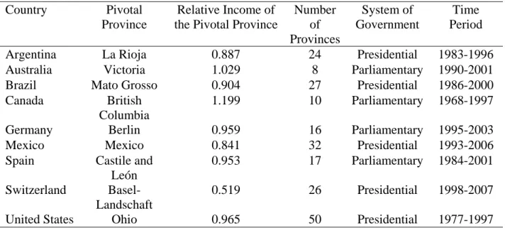
We begin by determining the pivotal province in each of the nine federations based on the provinces’shares of the representatives in the federal legislatures. As noted above, in many federations provinces, such as the United States, small states are over-representated because there is an upper house where representation is by province rather than by population. As well, in some federations, such as Argentina, small states are over-represented in the lower house. Thus to determine the pivotal province in each federation, we use data on the proportion of federal legislators that come from the province rather than its share of the population in each federation.
Table 1 shows the pivotal province in each of the nine federations, the pivotal province’s relative income, the number of provinces in the federation, whether the federation has a presidential or a parliamentary system, and the time period covered by the data. In most of these federations the pivotal provinces’per capita incomes are close to the national averages. They are above the national average in Australia and Canada. Only in Switzerland is the average income of the pivotal province, Basel-Landschaft, substantially below the national average. The data set consists of observation on transfers to 209 provinces in the nine federations based on average values of the variables over the time periods noted in Table 1. Of the 209 observations, 51 are from federations with parliamentary systems of government and 158 are from federations with presidential systems.
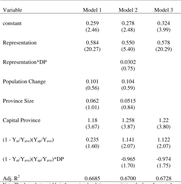
Table 2 shows the regression results where the dependent variable, Transfers, is the ratio of the province’s per capita transfer to the average per capita transfer for all provinces in the federation. In Model 1 we regress Transfers on Representation which is the ratio of the number of legislative seats per capita in a province to the average number of seats per province; Population Change which is the di¤erence between the relative population
of a province in the …rst year for which there are observations on grants and the relative population of the province approximately 10 years after the …rst observation; Province Size which is the ratio of the area of the province to the average area of the provinces in the federation; Capital Province which is a dummy variable that takes a value of one if the federal capital is located in the province; and Relative Incomes which is de…ned as (1 Yai=Yave)(Yap=Yave). The predicted sign of the estimated coe¢ cient for Relative Incomes is positive because an increase in province i’s relative income should reduce its relative transfer to the extent that the federation adopts a system of equalization grants given by (46) and an increase in the relative income of the pivotal province will increase (reduce) the relative transfer of a province if it is below (above) the average national income. In Model 1, the estimated coe¢ cients of the Representation variable and Capital Province are positive and statistically signi…cant at the one percent level. The estimated coe¢ cients of Population Change, Capital Province and Relative Incomes are positive but not statistically signi…cant. As previously noted, the allocation of transfers among provinces may be quite di¤erent under parliamentary and presidential systems of government because in a presidential system the representatives of the provinces may have more scope for forming coalitions with other provinces to capture more of the federal transfers. The model of the pattern of transfers that was developed in Sections 2 and 3 is more consistent with a parliamentary setting, where a particular political party can represent a set of regions with a common interest in setting the transfers to redistribute income in their favour. Based on this conjecture, we introduce a dummy variable, DP; which has a value of one if the country has a presiden-tial system. We hypothesize that under a presidenpresiden-tial system, the allocation of transfers is largely determined by the Representation variable, whereas under a parliamentary system, the Relative Incomes variable will determine the allocation of transfers. To capture the di¤erential e¤ects of Representation and Relative Incomes under parliamentary and presi-dential systems we multiply these variables by DP and add these two additional variables in Model 2. With this regression model, Representation is positive and highly signi…cant although the Representation*DP is not statistically signi…cant. However, the coe¢ cient of Relative Incomes increases in magnitude and is statistically signi…cant at the …ve percent
level and the Relative Incomes interacted with the DP is negative and statistically signi…cant at the 10 percent level. These results indicate that the Relative Incomes variable seems to have the predicted e¤ects on the relative transfers in parliamentary systems but little or no e¤ect on the distribution of transfers in presidential systems. Model 3 shows a simplied version of Model 2 by dropping Province Size, Population Change, and Representation*DP from the regression equation. The coe¢ cients of the remaining variables and their t statistics are little changed from the results obtained in Model 2.
6
Concluding Remarks
In this paper we have developed a political economy model that determines the size of the vertical …scal gap and the vertical …scal imbalances in the expenditures of the central govern-ment and subnational governgovern-ments. We have assumed that the system of transfers re‡ects the interests of voters located in di¤erent subnational governments across the country. We eschew the assumption of identical regions because regional variations in key economic vari-ables is one of the main reasons for federal forms of government exist. We have attempted to de…ne the concept of …scal balance, and its opposite, …scal imbalance, in terms of the allo-cation of spending at the two levels of government, rather than in terms of the conventional de…nition of a di¤erence between own source revenues and expenditures at the subnational level of government.
By making a strong assumption about the form of voters’utility functions, we are able to derive closed form expressions for the key …scal variables in the model. The basic model predicts that the residents in each province will vote for a combination of federal public services and transfers to the provinces such that they can achieve a …scal balance between spending at the federal level and at the provincial level. In general, this means that they would like to equalize the tax price of federal public services and provincial public services. Since the federal government is assumed to provide the same level of public service across the country, the residents of only one province can achieve a …scal balance. A simple majority voting model in the federal legislature predicts that this …scal balance will be achieved by the residents of the "pivotal province". The residents in provinces with lower average
incomes will perceive a federal imbalance, and they would like to see higher transfers to fund more provincial services and less spending on the federal public good. On the other hand, provinces with above average incomes will see a provincial imbalance in spending. The simple models outlined in Sections 2 and 3 indicate that a vertical …scal imbalance cannot be resolved through major voting in legislatures, but at least the imbalace will "balanced". While the objective of the paper is provide insights into the potential for resolving …scal imbalance by democratically elected governments, the model can also be used to predict the allocation of intergovernmental transfers in a federation. We have tested the key prediction of the model–that grants to reduce the vertical …scal imbalance between the two levels of government will be inversely related to the relative average income of the pivotal province– using time series data for Canada and cross-section data from nine federations. The key prediction of the model is rejected with the time series data for Canada, but the main prediction is veri…ed for the federations with parliamentary forms of government based on the cross-section data. The latter results then indicate that there are signi…cant di¤erences in the pattern of transfers to subnational governments under presidential and parliamentary systems. Further research may help to clarify and con…rm the di¤erences in the pattern of transfers to subnational governments with these two forms of government.
References
Becker, G. and C. Mulligan. 2003. "Deadweight Costs and the Size of Government." Journal of Law and Economics 46: 293-340.
Boadway, R. and J.-F. Tremblay. 2006. "A Theory of Fiscal Imbalance." FinanzArchiv 62(1): 1-27.
Boadway, R. and J.-F. Tremblay. 2010. "Mobility and Fiscal Imbalance." National Tax Jour-nal 63(4): 1023-1054.
Breton, A. 1996. Competitive Governments. Cambridge: Cambridge University Press. Casamatta, G., H. Cremer, and P. Pestieau. 2000. "Political Sustainability and the Design
of Social Insurance." Journal of Public Economics 75: 341-364.
Cremer, H., P. De Dedonder, D. Maldonado, and P. Pestieau. 2007. "Voting Over Type and Generosity of a Pension System When Some Individuals Are Myopic." Journal of Public Economics 91: 2041-2061.
Crémer, J. and T. Palfrey. 2000. Federal Mandates by Popular Demand. Journal of Political Economy, 108: 905-927.
Dahlby, B. and J. Roberts. 2010. “El Federalismo Fiscal en Canadá” in Federalismo Fis-cal. Experiencia Nacional y Comparada. edited by Pablo María Garat and Miguel Angel Asensio, Rubinzal-Culzoni Editores, pp. 295-313.
Dixit, A. and J. Londregan. 1998. Fiscal Federalism and Redistributive Politics. Journal of Public Economics 68: 153–180.
Dragu, T. and J. Rodden. 2010. "Representation and Redistribution in Federations." PNAS Early Edition, pp.1-4.
Hamilton, J. 1986. "The Flypaper E¤ect and the Deadweight Loss From Taxation." Journal of Urban Economics 19: 148-155.
Pereira, P. 1996. A Politico-Economic Approach to Intergovernmental Lump-Sum Grants. Public Choice 88: 185-201.
Porto, A. and P. Sanguinetti. 2001. Political Determinants of Intergovernmental Grants: Evidence from Argentina. Economics and Politics 13: 237-256.
Rodden, J. 2009. "Representation and Regional Redistribution in Federations" IEB’s World Report on Fiscal Federalism ’09 Institut d’Economia de Barcelona, pp. 68-77.
Sharma, Chanchal Kumar. 2012. “Beyond Gaps and Imbalances: Restructuring the Debate on Intergovernmental Fiscal Relations”, Public Administration— an International Quar-terly 90(1): 99-128.
Snoddon, T. and J-F. Wen. 2003. Grant Structure in an Intergovernmental Fiscal Game. Economics of Governance 4: 115-126.
Volden, C. 2007. "Intergovernmental Grants: A Formal Model of Interrelated National and Subnational Political Decisions." Publius 37: 209-243.
7
Appendix
To determine how the desired federal budget varies with average province income, we can write the left-hand side of (21) as (Rf; Yai) and the right-hand side as (Rf; Yai). Using this notation and taking the total di¤erential, we can obtain the following comparative static result: dRf dYai = Yai Yai f f (71) It can be shown that:
Yai = b4 Z2 ai 1 + + b > 0 (72) Yai = b + + b 3 g2 i < 0 (73) Rf = 1 + + b 3 g2 i + 3 G2 < 0 (74) Rf = ( + + b) X2 ai Yai Yave 2 + b 3 Z2 ai 1 + + b > 0 (75) and therefore: dRf dYai < 0 (76)
1981-82 1984-85 1987-88 1990-91 1993-94 1996-97 1999-00 2002-03 2005-06 2008-09 2 2.5 3 3.5 4 4.5
Figure 2
Cash Transfers to the Provinces as a
Percentage of GDP
Figure 1
The Detemination of the Preferred Level of the
Provincial Public Good
gi gi0 MB1gi MB2gi P2i P1i Y2i> Y1i
1981 1983 1985 1987 1989 1991 1993 1995 1997 1999 2001 2003 2005 2007 2009 0.8 0.85 0.9 0.95 1 1.05 1.1 1.15 1 Ontario Sask BC
Figure 3
Relative Average Income in the Pivotal
Province
0.9 0.95 1 1.05 1.1 Yap/Yave 2 2.5 3 3.5 4 4.5 T/YaveFigure 4
Transfer to GDP versus Relative Income of the
Pivotal Province
0.4 0.6 0.8 1 1.2 1.4 1.6 1.8 1 2 3 4 5 6 7 8 1981-82 0.6 0.7 0.8 0.9 1 1.1 1.2 1 2 3 4 5 6 7 8 9 1991-92 0.6 0.7 0.8 0.9 1 1.1 1.2 1.3 1.4 1.5 1 2 3 4 5 6 7 8 2001-02 0.7 0.8 0.9 1 1.1 1.2 1.3 1.4 1.5 1.6 1 2 3 4 5 6 7 8 2009-10
Figure 5
Ratio of Per Capita Transfers to National Average GDP
Per Capita versus the Provinces' Relative Per Capita
Table 1 Pivotal Provinces and Systems of Government for Nine Federations
Country Pivotal Province
Relative Income of the Pivotal Province
Number of Provinces System of Government Time Period
Argentina La Rioja 0.887 24 Presidential 1983-1996
Australia Victoria 1.029 8 Parliamentary 1990-2001
Brazil Mato Grosso 0.904 27 Presidential 1986-2000
Canada British Columbia
1.199 10 Parliamentary 1968-1997
Germany Berlin 0.959 16 Parliamentary 1995-2003
Mexico Mexico 0.841 32 Presidential 1993-2006
Spain Castile and
León
0.953 17 Parliamentary 1984-2001
Switzerland Basel-Landschaft
0.519 26 Presidential 1998-2007
Table 2 Regression Results From Cross-Section Data
Variable Model 1 Model 2 Model 3
constant 0.259 0.278 0.324 (2.46) (2.48) (3.99) Representation 0.584 0.550 0.578 (20.27) (5.40) (20.29) Representation*DP 0.0302 (0.75) Population Change 0.101 0.104 (0.56) (0.59) Province Size 0.062 0.0515 (1.01) (0.84) Capital Province 1.18 1.258 1.22 (3.67) (3.87) (3.80)
(1 - Yai/Yave)(Yap/Yave) 0.235 1.141 1.122
(1.60) (2.07) (2.07)
(1 - Yai/Yave)(Yap/Yave)*DP -0.965 -0.974
(1.70) (1.75)
Adj. R2 0.6685 0.6700 0.6728
Note: The dependent variable is the province’s relative per capita transfer from the central government. The number of observations is 209. Absolute values of t statistics are shown in parentheses.