View of Unidimensionality in the Rasch model: how to detect and interpret

UNIDIMENSIONALITY IN THE RASCH MODEL: HOW TO DETECT AND INTERPRET

E. Brentari, S. Golia

1. INTRODUCTION

The concept of unidimensionality is frequently defined as a single latent trait be-ing able to account for the performance on items formbe-ing a questionnaire. It repre-sents a fundamental requirement when an item response theory model or a Rasch model is used in order to obtain a measurement for the latent trait of interest.

In literature, there are many approaches for assessing the dimensionality of item response data. Among these, the first is based on prior testing which uses, for example, the linear factor analysis, or the Martin-Löf test (Martin-Löf, 1970, Gustafsson, 1980 and Glas and Verhelst, 1995 and extension to polytomous i-tems, Christensen, Bjorner, Kreiner, and Petersen, 2002). The latest makes use of a conditional approach with no distributional assumptions about the latent vari-able and requires that the dimensional composition is known, so that the items fall into two subsets such that all items in the same subset represent the same di-mension.

A second approach is based on a post-hoc testing such as principal compo-nents analysis of residuals and item fit statistics, whereas a third approach on nonparametric procedures such as, for example, the dimtest (Stout, 1987). Dimtest is a creative and mathematically ambitious attempt to assess unidimensionality and requires to partition the test items into three subtests: AT1, a “unidimen-sional” subtest, AT2, a subtest with the same difficulty distribution as AT1, and PT, a subtest used for partitioning person abilities. Then some calculations pro-duce Stout's T statistic that assesses departure from essential unidimensionality.

In the present paper the attention will be focused on detecting unidimensional-ity by using principal components analysis of Rasch residuals (Bond and Fox, 2007) and item fit statistics.

This study investigates, making use of simulate data, how principal compo-nents analysis and fit statistics work when data exhibit multi-dimensionality. Two different sources of bi-dimensionality are taken into account. The first is due to the presence of two distinct latent constructs. The second is due to two groups of items, all related to a unique latent trait, one of which is composed by highly

cor-related items. The application of the simulative results to the data-base coming from the job satisfaction section of the first national survey concerning the social services sector carried out in Italy (Borzaga and Musella, 2003) permits to con-clude that the second trait, reviled by the principal components analysis of Rasch residuals, can be treated as a sub-dimension of job satisfaction (two variables measure the same aspect of job satisfaction), rather than a distinct second trait not related to the main trait.

The paper is organized as follows. Section 2 reviews the Rasch model while section 3 reports the results of the simulative study for both uni- and bi-dimensional data. In section 4 data from the and job satisfaction section the na-tional survey is analyzed.

2. THE RASCH MODEL

The Rasch Model (RM) (Rasch, 1960), is a family of measurement models which converts raw scores into linear and reproducible measurement. Its distinguishing characteristics are: separable person and item parameters, sufficient statistics for the parameters and conjoint additivity. These features enable specifically objective comparisons of persons and items and allow each set of model parameters to be conditioned out of the estimation procedure for the others.

It requires unidimensionality, which means that all items forming the questionnaire measure only a single construct, i.e. the latent trait under study, and local independence, which requires that, conditional to the latent trait, the response to a given item is independent from the responses to the other items in the questionnaire.

If the data fit the model, then the measures produced applying the RM to the sample data are objective and expressed in logits (logarithm of odds) which has the property of maintaining the same size over the entire continuum.

According to the RM, the probability that a person n answers in a given way, say x, to the item i depends on subject ability and how difficult the item is to en-dorse. For polytomously scored items, that is when there are m+1 possible or-dered response categories for each item (coded as x = 0, 1,..., m), following the

Rating Scale Model (Andrich, 1978), this probability is given by:

0 0 0 exp ( ) ( ) exp ( ) x n i j j ni _{m k} n i j k j x P X x k β δ τ β δ τ = = = ⎧ ⎫ ⎪ _{− −} ⎪ ⎨ ⎬ ⎪ ⎪ ⎩ ⎭ = = ⎧ ⎫ ⎪ _{− −} ⎪ ⎨ ⎬ ⎪ ⎪ ⎩ ⎭

∑

∑

∑

where τ0 = . 0 βn identifies the ability of person n, δi the mean difficulty of item i and τj, called threshold, is the point of equal probability of categories j-1 and j. Thresholds add up to zero, i.e.

1 0 m j j τ = =

∑

In order to evaluate the accord between the model and the data and verify the model assumptions, it is possible to use specific tools for diagnostic checking based on residual analysis. The residual y is given by the difference between ni the observed and expected answer to the item i by the subject n (i.e.

( ) ni ni ni y =x −E X , with 0 ( _ni) m ( _ni ) k E X k P X k =

=

∑

residuals z are calculated as _ni z_ni = y_ni Var X( _ni). Each residual shows a piece of information about the quality of data. Large residuals raise doubts concerning the match between model and data (Wright and Masters, 1982).

In the present paper the outfit and infit mean square statistics and the principal com-ponent analysis (PCA) are considered, in order to evaluate the unidimensionality

as-sumption.

The outfit and infit mean square statistics are, respectively, defined as:

2 1 1 N i ni n u z N = =

∑

∑

∑

∑

∑

Outfit statistic u measures the average mismatch between model and data and is i sensitive to extreme values. Infit statistic v is more sensitive to pattern of re-_i

sponses to items targeted on the subject and vice versa. Their expected value is 1 and they take values from 0 to infinity. Values near 1 indicate little distortion of the measurement system; values less than 1 indicate observations which are too predictable while values greater than 1 indicate unpredictability and un-modelled noise. Item fit statistics help in identifying problematic items.

The purpose of the un-rotated principal component analysis on standardized residuals used in the Rasch context is not to find shared factors. The underline hypothesis is that there is only one dimension, called the Rasch dimension, captured by the model so that the residuals do not contain other significant dimensions. Hence, the purpose is to verify the absence of other significant dimensions. The attention is focused on the eigenvalues of PCA on Rasch residuals.

3. SIMULATION STUDY

The present section reports the results of the analysis of uni- and bi-dimensional data. The bi-bi-dimensionality is induced adopting two different meth-ods; the first lies in identifying two groups of items which require two different abilities whereas the second in releasing the local independence assumption for a

1 _{It must be noted that ( )}

ni

E X is an estimated expected value due to the fact that the parame-ters in (1) are unknown and have to be estimated.

group of items so that the identification of two traits which are related to each other (but do not require different abilities) becomes possible. The attention is focus on the behavior of the size of the eigenvalues related to the factors identi-fied with the PCA and the infit and outfit mean square statistics.

The RM used in the study is the Rating Scale model (1) with fifteen items, five common thresholds, fixed as [-1, -0.5, 0, 0.5, 1], and three different sizes for the simulated data sets are considered, that is n = 100, 500, 1000.

In order to have benchmarks for the first two eigenvalues of PCA on Rasch residuals and the outfit and infit mean square statistics, unidimensional data sets are simulated, making use of the parametric formulation of the Rasch response probability (1); the response given by the subject n to the item i is obtained as fol-lows. First, for all the categories, the response probabilities and their cumulative sum are computed. Then, a random number rn is chosen from a uniform distri-bution on the interval [0,1] and compared with the cumulative sum; the first cate-gory with cumulative sum larger than rn is assigned to the response. In the simu-lations the subject ability, i.e. the subject’s level of latent trait, is drawn from a standard normal distribution and the mean item difficulties are chosen equal to [-2.0993, -1.4023, -0.7288, -0.5797, -0.4789, -0.3994, -0.2591, -0.1740, 0.3857, 0.4206, 0.67, 0.9938, 1.0179, 1.2588, 1.3747].

In the calibration procedure the analysis was performed by setting the mean of item difficulty estimates to 0.0 logits and by using the (unconditional) maximum likelihood estimation method2_.

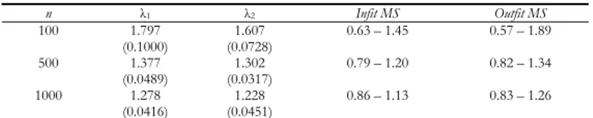
Table 1 displays the mean value and the corresponding standard error of the first two eigenvalues λ1 and λ2 of PCA on Rasch residuals calculated on 100 data-sets.

The reference values for the infit and outfit mean square statistics, shown in Table 1, are obtained as follows. For each data set the minimum and maximum infit and outfit are recorded so that four series of 100 values are available. For each minimum and maximum a 95% empirical confidence interval is computed. The infit mean square (outfit mean square) range is defined using the lower bound of the minimum empirical confidence interval and the upper bound of the maximum empirical confidence interval.

TABLE 1

Reference values for the first two eigenvalues of PCA on Rasch residuals and the outfit and infit mean square statistics

n λ1 λ2 Infit MS Outfit MS 100 1.797 (0.1000) (0.0728) 1.607 0.63 – 1.45 0.57 – 1.89 500 1.377 (0.0489) (0.0317) 1.302 0.79 – 1.20 0.82 – 1.34 1000 1.278 (0.0416) (0.0451) 1.228 0.86 – 1.13 0.83 – 1.26

2 _{The analysis was performed using the Winsteps 3.63 software (Linacre, 2006). It must be noted}

that Winsteps drops persons and items with extreme scores (zero and perfect scores). Nevertheless, no items and only few persons got extreme scores.

It should be noted that the size n = 100 is rather small and the estimates are less stable; anomalous behaviors come out even when the data are generated ap-plying unidimensional RM.

3.1. Case 1

The first method with which the bi-dimensionality is induced, lies in defining two groups of items that require two different levels of ability. The first set of ability levels is drawn from a standard normal random variable X. The second one, following Smith (2002), is drawn from a normal random variable Yc which depends on X and on a second standard normal random variable Y, independent

of X, according to the relation _{( 1} 2 ₎

c c c

Y = ⋅a X + −a Y S⋅ ⋅ +M , where Mc and

Sc are respectively the mean and the standard deviation of the Yc distribution. The

Yc is correlated with X at the specific level a, with a ∈(0,1).

In the simulation study Mc = 0, Sc = 1 and a is set equal to 0.2 and 0.7. The ability distribution X is used to generate the responses to 13 items with mean dif-ficulty [-1.7356, -1.424, -0.8764, -0.625, -0.3668, 0.0234, 0.1603, 0.4374, 0.7089, 1.5953, 2.1025, -1.5234, -1.3707], whereas the ability distribution Yc is used to generate the responses to the last two items with mean difficulty [1.1283, 1.7658]. The simulated data are obtained applying the response probability (1), according to the scheme described at the beginning of section 3.

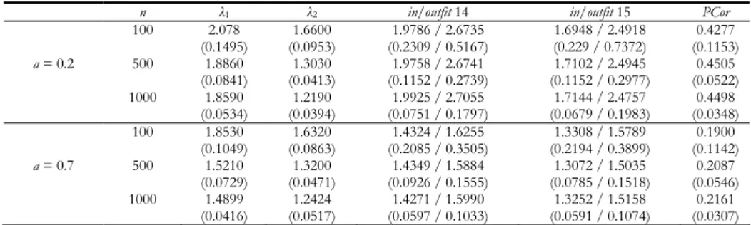
Table 2 reports the mean value, calculated on 100 simulated data sets, of the first two eigenvalues (λ₁ and λ₂), the infit and outfit mean square statistics of the last two items and the Pearson correlation (PCor, computed between residuals across all subjects who responded to both items) for the couple 14-15.

TABLE 2

Mean value, calculated on 100 simulated data sets, of the first two eigenvalues, the infit and outfit mean square statistics of items 14 and 15 and the Pearson correlation for the couple 14-15; in parenthsis the standard errors

n λ1 λ2 in/outfit 14 in/outfit 15 PCor

100 2.078 (0.1495) (0.0953) 1.6600 (0.2309 / 0.5167) 1.9786 / 2.6735 (0.229 / 0.7372) 1.6948 / 2.4918 (0.1153) 0.4277 a = 0.2 500 1.8860 (0.0841) (0.0413) 1.3030 (0.1152 / 0.2739) 1.9758 / 2.6741 (0.1152 / 0.2977) 1.7102 / 2.4945 (0.0522) 0.4505 1000 1.8590 (0.0534) (0.0394) 1.2190 (0.0751 / 0.1797) 1.9925 / 2.7055 (0.0679 / 0.1983) 1.7144 / 2.4757 (0.0348) 0.4498 100 1.8530 (0.1049) (0.0863) 1.6320 (0.2085 / 0.3505) 1.4324 / 1.6255 (0.2194 / 0.3899) 1.3308 / 1.5789 (0.1142) 0.1900 a = 0.7 500 1.5210 (0.0729) (0.0471) 1.3200 (0.0926 / 0.1555) 1.4349 / 1.5884 (0.0785 / 0.1518) 1.3072 / 1.5035 (0.0546) 0.2087 1000 1.4899 (0.0416) (0.0517) 1.2424 (0.0597 / 0.1033) 1.4271 / 1.5990 (0.0591 / 0.1074) 1.3252 / 1.5158 (0.0307) 0.2161

The coefficient a measures the degree of correlation between the two abilities

X and Yc; a = 0.2 indicates a low degree of correlation, therefore the two abilities are sparely related and the two groups of items describe two well-separated latent variables. Under this hypothesis, the first eigenvalue λ1 takes values bigger than

sizes n, λ1 assumes a value close to 2 and this indicates that the implied

dimen-sion in the data has the strength of around two items. Moreover, the analysis of the infit and outfit mean square statistics points out that these two items are problematic and inconsistent with the dominant latent trait described by the first 13 items. Therefore, the combined use of these two indicators (λ₁ and fit statis-tics) allows to clearly identify the items forming a second latent trait which is dif-ferent from the dominant one and sparely related.

Similar conclusions can be drawn if a = 0.7, that is when the two abilities are strongly related and the two groups of items describe two latent traits that are not so different. However, the sign of multidimensionality represented by λ1 is less

marked. 3.2. Case 2

The second method with which the bi-dimensionality is induced, lies in impos-ing a strong relationship within a group of items so that the identification of two traits which are related to each other, but do not require different abilities, be-comes possible.

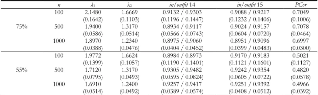
A unique unit normal ability distribution and a set of 15 items with mean diffi-culty [-2.0993, -1.4023, -0.7288, -0.5797, -0.4789, -0.3994, -0.2591, -0.174, 0.3857, 0.4206, 0.67, 0.9938, 1.0179, 1.2588, 1.3747] are used in order to simulate the re-sponses to all the 15 items applying the response probability (1), according to the scheme described at the beginning of section 3. The last item, with mean diffi-culty equal to 1.3747, is modified so that the 75% (and the 55%) of the responses are equal to the ones given to the item with mean difficulty equal to 1.2588.

Table 3 reports the mean value, calculated on 100 simulated data sets, of the first two eigenvalues, the infit and outfit mean square statistics of the last two items and the Pearson correlation for the couple 14-15.

TABLE 3

Mean value, calculated on 100 simulated data sets, of the first two eigenvalues, the infit and outfit mean square statistics of items 14 and 15 and the Pearson correlation for the couple 14-15; in parenthesis the standard errors

n λ1 λ2 in/outfit 14 in/outfit 15 PCor

100 2.1480 (0.1642) (0.1103) 1.6669 (0.1196 / 0.1447) 0.9132 / 0.9303 (0.1232 / 0.1406) 0.9088 / 0.9217 (0.1006) 0.7049 75% 500 1.9400 (0.0586) (0.0514) 1.3170 (0.0566 / 0.0743) 0.8934 / 0.9117 (0.0604 / 0.0720) 0.9024 / 0.9157 (0.0464) 0.7078 1000 1.8970 (0.0388) (0.0476) 1.2340 (0.0404 / 0.0452) 0.8975 / 0.9060 (0.0399 / 0.0483) 0.8951 / 0.9096 (0.0300) 0.6997 100 1.9772 (0.1399) (0.1057) 1.6624 (0.1190 / 0.1401) 0.8984 / 0.8973 (0.1121 / 0.1601) 0.9170 / 0.9183 (0.1127) 0.5021 55% 500 1.7120 (0.0795) (0.0493) 1.3170 (0.0595 / 0.0824) 0.9305 / 0.9482 (0.0605 / 0.0722) 0.9242 / 0.9354 (0.0578) 0.4820 1000 1.6910 (0.0514) (0.0492) 1.2400 (0.0389 / 0.0574) 0.9257 / 0.9417 (0.0408 / 0.0512) 0.9251 / 0.9392 (0.0392) 0.4966

With respect to the first percentage of equal responses (75%) and for all the different sizes of the data, the first eigenvalue assumes values around 2, higher

than the one that may be found when the unidimensionality assumption holds, nevertheless the infit and outfit mean square statistics of the two items forming the second dimension, do not indicate any problematic behaviour. Pearson corre-lation for the couple 14-15 is very high, pointing out a strong residual correcorre-lation between the two items. The multidimensionality found in Case 2 has characteris-tics different from what was found in Case 1, that is the second dimension is so closely connected to the dominant latent trait that can be viewed as a sub-dimension rather than a separate trait.

Similar results come out when the percentage of equal responses is set to 55%. 4. REAL DATA

The present section contains the results of the analysis of a real data set com-ing from the satisfaction section of the first national survey concerncom-ing the social services sector, carried out in Italy (Borzaga and Musella, 2003). It includes items that represent the principal facets that can be found in some of the most popular job satisfaction instruments, such as appreciation, job conditions, coworkers or pay.

For each item, respondents were asked to indicate how satisfied they were with it, choosing a score from 1 (very dissatisfied) to 7 (highly satisfied). Only workers employed in Social Cooperatives were considered so that the size of the dataset is 541.

A preliminary analysis suggested to merge together the second and the third categories, obtaining a 6-level Likert response scale for each item and did not consider the item relation with voluntary workers (relevant only for a small subset of workers who were in contact with voluntary workers ) so that 13 items were in-cluded in the analysis. Moreover, Brentari and Golia (2008) showed that, for this data set, the Rating Scale model is the more appropriate to estimate the worker job satisfaction and the items difficulty (that is how difficult it was, on average, for the group of workers to endorse each item).

What we expect from the analysis of a real unidimensional database is that a dominant dimension exists with the possible presence of minor dimensions and that this dominant dimension is so strong that the trait estimates are not affected by the presence of the smaller dimensions.

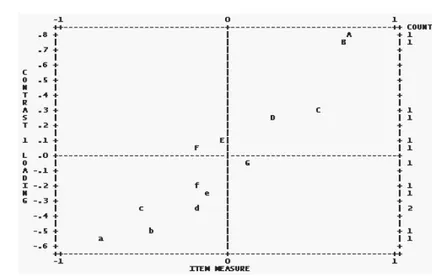
Figure 1 displays the results of the un-rotated principal component analysis to the standardized residuals. Letters “A,B,C,...” and “a,b,c,...” identify items with the most opposed loadings.

The residual component has first eigenvalue equal to 2.3 and it seems that it is explaining more than random variation. Items 9 (B in Figure 1), career promotions

achieved up to this moment in this organization, and 10 (A in Figure 1), promotion prospects,

are found responsible for the extra dimension.

The values of the infit and outfit mean square statistics of these two items are, respectively, 1.02 and 1.00 for item 9, 1.03 and 1.04 for item 10 and they are con-sistent with the values expected for these fit statistics. Moreover, the value of the

Figure 1 – Standardized residual contrast 1 plot; B corresponds to item 9 and A to item 10.

Pearson correlation coefficient for this couple of items is rather high, that is 0.52. The conclusion could be that the second trait pointed out by the analysis can be treated as a sub-dimension of the latent trait of interest (i.e. worker job satisfac-tion) rather than a distinct second trait not related to the main trait.

5. CONCLUSIONS

In the present paper the attention has been focused on detecting unidimen-sionality using principal components analysis of Rasch residuals and item infit and outfit mean square statistics. Two different sources of multidimensionality have been taken into account: two distinct latent constructs and a unique latent trait described by two groups of items, one of which composed by highly corre-lated items.

The simulation study highlighted the necessity to evaluate jointly the results of the PCA and the fit statistics in order to identify the nature of the multidimen-sionality, when the data are not unidimensional.

Preliminary analysis related to other combinations of items forming two di-mensions and “questionnaires” composed by a higher number of items, suggests that the results obtained in section 3 are rather general.

Dipartimento Metodi Quantitativi EUGENIOBRENTARI

Università degli Studi di Brescia SILVIAGOLIA

AKNOWLEDGEMENTS

The authors wish to thank M. Carpita for useful and valuable discussions and the anonymous reviewer for her/his useful comments.

REFERENCES

D. ANDRICH, (1978), A rating formulation for ordered response categories, “Psychometrika”, 43, pp.

561-573.

T.G. BOND, C.M. FOX, (2007), Applying the Rasch Model. Fundamental measurement in the human

sciences, snd Edition, Erlbaum, Mhawah NJ.

C. BORZAGA, M. MUSELLA, (2003), Produttività ed efficienza nelle organizzazioni nonprofit. Il ruolo dei

lavoratori e delle relazioni di lavoro, Edizioni31, Trento.

E. BRENTARI, S. GOLIA, (2008), Measuring Job Satisfaction in the Social Services Sector with the Rasch

Model, “Journal of Applied Measurement”, 9 (1), pp. 45-56.

K.B. CHRISTENSEN, J.B. BJOMER, S. KREINER, J.H. PETERSEN, (2002), Testing unidimensionality in

poly-tomous Rasch models, “Psychometrika”, 67 (4), pp. 563-574.

C.A.W. GLAS, N.D. VERHELST, (1995), Testing the Rasch model, in G.H. FISCHER, I.W. MOLENAAR

(Eds.), Rasch models - foundations, recent developments, and applications, Springer-Verlag.

J.E. GUSTAFSSON, (1980), Testing and obtaining fit of data to the Rasch model, “British Journal of

Mathematical and Statistical Psychology”, 33, pp. 205-233.

J. HATTIE (1985), Methodology review: assessing unidimensionality of tests and items, “Applied

Psy-chological Measurement”, 9 (2), pp. 139-164.

J.M. LINACRE (2006), WINSTEPS Rasch measurement computer program, Chicago:

Win-steps.com.

P. MARTIN-LÖF, (1973), Statistiska modeller [Statistical models.] Anteckningar från seminarier

lasåret 1969-1970, utarbetade av Rolf Sundberg. Obetydligt ändrat nytryck, October 1973. Stockholm: Institütet för Försäkringsmatemetik ochMatematisk Statistisk vid Stockholms Universitet.

G. RASCH, (1960), Probabilistic models for some intelligence and attainment tests, Copenhagen, The

Danish Institute of Educational Research.

R.M. SMITH, (1996), A comparison of methods for determining dimensionality in Rasch measurement,

“Structural Equation Modeling”, 3, pp. 25-40.

JR. E.V. SMITH, (2002), Detecting and evaluating the impact of multidimensionality using item fit

statis-tics and principal component analysis of residuals, “Journal of Applied Measurement”, 3, pp. 205-231.

W.F. STOUT, (1987), A nonparametric approach for assessing latent trait unidimensionality,

“Psycho-metrika”, 52, pp. 293-325.

B.D WRIGHT, G.N. MASTERS, (1982), Rating Scale Analysis, MESA Press, Chicago.

SUMMARY

Unidimensionality in the Rasch model: how to detect and interpret

Unidimensionality, that is the items in a questionnaire measure only a single construct, is a fundamental requirement for the Rasch model. The paper deals with the detection of unidimensionality making use of principal components analysis of residuals and item fit statistics. Simulated bi-dimensional data sets are analized in order to find regolarities in the behavoiur of these statistical tools. The results are applied to a real database coming from the satisfaction section of the first national survey concerning the social services sec-tor carried out in Italy.