Col.lecció d’Economia E17/360
Anatomizing the Mechanics of Structural
Change
Jaime Alonso-Carrera
María Jesús Freire-Serén
Xavier Raurich
UB Economics Working Papers 2017/360
Anatomizing the Mechanics of Structural
Change
Abstract:We characterize several possible mechanisms of structural change by using
a general multisector growth model, where preferences and technologies are not parameterized. In this generic set up, we derive the growth rates of sectoral employment shares at the equilibrium. We find that the economic fundamentals governing structural change in the sectoral employment shares are: (i) the income elasticities of the demand for consumption goods; (ii) the Allen-Uzawa elasticities of substitution between consumption goods; (iii) the capital income shares in sectoral outputs; and (iv) the elasticity of substitution between capital and labor in each sector. These fundamentals determine the effect that the growth rates of aggregate income, relative prices, rental rates and technological progress have on structural change. Finally, we estimate the aforementioned fundamentals to develop an accounting exercise that quantifies the contribution of each mechanism to the U.S. structural change.
JEL Codes: O11, O41,O47.
Keywords: Structural change, structural transformation, non-homothetic preferences, sectoral productivity.
Jaime Alonso-Carrera Universidade de Vigo María Jesús Freire-Serén Universidade de Vigo Xavier Raurich
Universitat de Barcelona
Acknowledgements: Financial support from the Government of Spain and FEDER
through grants ECO2015-66701-R and ECO2015-68367-R (MINECO/FEDER); and the Generalitat of Catalonia through grant SGR2014-493 is gratefully acknowledged. This paper has benefited from comments by participants in the Workshop on Structural Change and Economic Growth at University of Barcelona and III Navarre-Basque Country Macroeconomic Workshop.
1. Introduction
The process of economic growth and development exhibits structural change as one of the most robust features. Developed countries have experimented a secular shift in their allocation of employment, output and expenditure across the sectors of agriculture, manufactures and services. Figure 1 shows evidence of this long run trend in the U.S. economy. We observe that the production valued added, labor and expenditure on consumption valued added have continuously shifted from agriculture and manufactures to services during the period from 1947 to 2005. In particular, employment shares in agriculture and manufactures have monotonically decreased during this period, whereas the employment share in serviceses has increased path. The valued added and expenditure shares qualitatively replicate the shape of the dynamics followed by the employment shares. Figure 2 also shows the dynamic path followed by the capital income shares, the total factor productivity (henceforth, TFP) indexes, the prices of the three sectoral outputs and the ratio between the rental rate of labor and the rental rate of capital in these three sectors. We easily observe that the relative price of agriculture in terms of manufactures has decreased substantially, whereas the relative price of services has instead grown up during the sample period. Furthermore, the dynamic behavior of the other three magnitudes also clearly di¤ers across the three sectors. Especially, we must emphasize that the accumulated growth rate of TFP has been much larger in agriculture than in manufactures and services. The changes in the variables displayed in Figure 2 together with economic growth are the mechanisms that, according to the literature, drive the patterns of structural change shown in Figure 1.1 Our aim is to identify and estimate the deep fundamentals that measure the contribution that each of these economic mechanisms has on structural change.
[Insert Figures 1 and 2]
Recently, there is a renewed and growing interest in analyzing what are the possible economic factors driving the sustained process of structural transformation observed in the data. This literature has distinguished between demand-based and supply-based mechanisms of structural change. On the one hand, structural change in a growing economy is driven by income e¤ects due sectoral di¤erences in income elasticities of consumption demand (i.e., when preferences are non-homothetic). These factors have been studied by, among others, Echevarria (1997), Laitner (2000), Kongsamunt et al. (2001), Caselli and Coleman (2001) or Foellmi and Zweimüller (2008). On the other hand, the aforementioned literature also …nds some supply factors that cause structural change through a substitution e¤ect. One of these contributions is in Ngai and Pissarides (2007), who formalize the original idea of Baumol (1967) to explain structural change as a consequence of a sectoral-biased process of technological change. Alternatively, Acemoglu and Guerrieri (2008) explain this substitution e¤ect behind structural change by the interaction between sectoral production functions with di¤erent capital intensities and capital deepening. Finally, Alvarez-Cuadrado et al. (2013) point out that di¤erences in the capital-labor substitution across sectors are also a candidate for a supply factor of structural transformation.
1See, for example, Herrendorf et al. (2014) for an extensive review of the literature on structural
However, there is little consensus in the literature on the relative importance of the suggested mechanisms for explaining the observed structural transformation. There are some applied studies that analyze the accuracy of some mechanisms to explain the observed structural change. In particular, Dennis and Iscan (2009) quantitatively decompose U.S. reallocation of labor out of agriculture sector into a demand-side e¤ect, an e¤ect from sectorally biased technological change and an e¤ect from di¤erential sectoral capital deepening. Herrendorf et al. (2013) analyze the ability of income and substitution e¤ects to explain U.S. structural change by focusing on how restrictions on preference parameters a¤ect the …t of expenditure rates. Herrendorf et al. (2015) assess how the properties of technology a¤ect the reallocation of production factors across sectors. Moro et al. (2015) study how a model with non-homothetic preferences and home production …t the observed patterns of structural change. Finally, Sweicki (2013) goes further in studying the importance of several mechanisms. He simulates a parametrized general equilibrium model to quantify in a large set of countries the contribution to structural change of four particular mechanisms: (i) sector-biased technological change, (ii) non-homothetic preferences, (iii) international trade, and (iv) intersectoral wedges between sectoral rental rates. However, the analysis in all these papers is based on particular assumptions on the functional forms of both technologies and preferences. Obviously, these assumptions may bias the measure of the contribution of the di¤erent mechanisms of structural change. Therefore, a uni…ed framework of analysis that combines several mechanisms of structural change in a general model seems necessary to obtain appropriate measures of the contribution of each mechanisms. The goal of this paper is to construct the aforementioned uni…ed framework of analysis. In particular, we …rst characterize the di¤erent mechanisms of structural change in a close economy by using a generic framework, i.e., a model with the minimum set of assumptions and without parametrizing preferences and technologies. We derive the growth rates of sectoral employment shares at the equilibrium of this generic set up. In this way, we are able to identify the economic fundamentals that are behind structural change. We …nd that those crucial fundamentals are: (i) the income elasticities of the demand for consumption goods; (ii) the Allen-Uzawa elasticities of substitution between consumption goods; (iii) the capital income shares in sectoral outputs; and (iv) the elasticity of substitution between capital and labor in each sector. These fundamentals crucially determine the importance of the growth rates of aggregate income, relative prices, rental rates and technological progress for structural change. Obviously, our expression for the process of structural change can be particularized to all of the proposals provided by the existing literature. In the paper, we illustrate how these particular mechanisms can be interpreted and explained with our general condition for structural change.
We also develop an accounting exercise to quantify the contribution of each mechanism to the U.S. structural change. To this end, we …rst estimate the aforementioned fundamentals determining the weight of each mechanism. We show that the following mechanisms have had a large e¤ect on the dynamics of sectoral employment shares in the US economy: (a) the income e¤ects caused by both the growth of income and the changes in relative prices; and (b) the demand substitution and technological substitution e¤ects caused by the variation of prices derived from sectoral-biased technological progress, capital deepening and sectoral di¤erences in
capital-labor substitution. However, they have worked in di¤erent directions. The dynamics of employment out of agriculture are mainly driven by the technological substitution e¤ects, whereas the push on of employment to the service sector is mainly caused by the income e¤ects. Moreover, all of these e¤ects have varied along time because of the time-varying nature of the fundamentals.
Our analysis has clear contributions. It …rst o¤ers a uni…ed framework to study structural change and to isolate the economic fundamentals that we should take into account in characterizing this process. As a consequence, from our general expression for the sectoral reallocation of labor, we can derive the conditions that these fundamentals should satisfy to …t the observed process of structural change. This exercise can be done either by isolating an individual mechanism or by considering the interaction among several mechanisms. As was mentioned before, in the paper we make this exercise for each of the mechanisms already considered by the literature. We then use our general framework to interpret the conditions for structural transformation provided by this literature.
On the other hand, our analysis contributes to introduce discipline in building multisector growth model for the economic analysis. To consider all of the mechanisms with a signi…cant contribution to the observe structural change, as well as to identify the fundamentals that determine this contribution, seems a necessary requirement to derived unbiased conclusions on the macroeconomic e¤ects of structural shocks like, for instance, …scal policy reforms. These shocks may distort the economy by means of di¤erent mechanisms of structural change and, in addition, they may even alter substantially the contribution of these mechanisms. Therefore, it is only possible to derive the entire e¤ect of the shocks by considering all of the mechanisms in the same uni…ed model. Our accounting exercise o¤ers one of the …rst serious try in this direction, although some other mechanisms may be still skipped.2
The rest of the paper is organized as follows. Section 2 presents the theoretical framework used by the analysis. Section 3 derives the growth rates of the sectoral shares of employment at the equilibrium and characterizes the mechanisms driving structural change in this general setting. Section 4 revisits the recent literature on structural change to show how our general formulation can be particularized in these contributions. Section 5 performs an empirical analysis to disentangle the relative importance of the derived mechanisms for the structural change observed in US data. Section 6 includes some concluding remarks. Finally, the details of some mechanical analysis are included in the appendix.
2. Theoretical framework
We consider a continuous time, close economy composed of m productive sectors. We interpret sector m as the one producing manufactures that can be devoted to either consumption or investment, whereas the other m 1 sectors produce pure consumption goods. Firms in each sector i operate under perfect competition by using the following
2
For instance, we do not consider the e¤ect of international trade in the process of structural change. Uy et al. (2013), Sweicki (2013) and Teignier (2014) show that this may be an important channel to explain the observed structural change.
sector-dependent production function:3
Yi= Fi(siK; AiuiL) ; (2.1)
where Yiis the output produced in sector i; siis the share of total capital, K; employed in sector i; ui is the share of total employment, L; in sector i; and Ai measures the e¢ cient units of employment in sector i: We assume that
_ Ai Ai
= i; (2.2)
that is, the e¢ cient units of labor grow at the rate i; which can be di¤erent across sectors. Hence, technological progress can be either sectorally biased or unbiased.
We assume that the sectoral production functions are increasing in both capital and e¢ cient units of labor, they exhibit decreasing returns in each of these arguments, and they are linearly homogenous in both arguments. We can then express sectoral production in e¢ cient units of labor as
yi = fi(ki) ; (2.3)
where yi = Yi=AiuiL is the output in e¢ cient units of labor in sector i; and ki = siK=AiuiL measures capital intensity in sector i: Given the properties of the sectoral production functions, we know that fi0(ki) > 0 and f
00
i (ki) < 0:
Finally, perfect competition implies that each production factor is paid according to its marginal productivity. Hence, the following conditions hold:
ri= pifi0(ki) ; (2.4)
and
wi= piAi fi(ki) fi0(ki) ki ; (2.5) where riand wi are the rental rates of capital and labor, respectively, in sector i: These rental rates can di¤er across sectors. This may be the case, for instance, if there exist some costs of moving production factors across sectors or intersectoral distortions and frictions (see, e.g., Caselli and Colleman, 2001; Buera and Kaboski, 2009; Sweicki, 2013; or Alonso-Carrera and Raurich, 2016). We denote by pi and !i = wi=ri the price of commodity Yi and the rental rate ratio in sector i, respectively. By combining (2.4) and (2.5), we conclude that the stock of capital in e¢ cient units of labor ki is an implicit function of the rental rate ratio !i and of the e¢ cient units of labor Ai: Hence, we can write ki = i(!i; Ai) ; with @ki @!i = [f 0 i(ki)] 2 Aifi(ki) fi00(ki) > 0; and @ki @Ai = fi0(ki) [fi(ki) fi0(ki) ki] Aifi(ki) fi00(ki) < 0; 3
which follows from the properties of sectoral production functions. Note that the relation between capital in e¢ cient units of labor and the rental rate ratio is sectoral dependent because so are the production functions.
For our analysis, it will be also useful to characterize the …rms’ optimal behavior by the following fundamentals of sectoral structure of production: (i) the share of capital income in output from sector i; that we denote by i; and (ii) the elasticity of substitution between capital and labor in sector i; that we denote by i. By using (2.3), (2.4) and (2.5), together with the de…nition of the rental rate ratio !i, we obtain, after some simple algebra, that
i = riki piyi = f 0 i(ki) ki fi(ki) ; (2.6) and i= @ki @!i !i ki = (1 i) f 0 i(ki) f00 i (ki) ki : (2.7)
Observe that these two fundamentals i and i can be di¤erent across sectors. In this case, the prices pi depend not only on the exogenous technical change, but they are also endogenously determined by capital accumulation.
This economy is populated by a unique in…nitely-lived representative consumer. This consumer obtains income from renting capital and labor to …rms. This income is devoted to either consumption or investment. Therefore, his budget constraint is
m X i=1 (riki+ wiuiL) = _K + (1 ) K + m X i=1 pici; (2.8)
where ci is the consumption demand of the commodity produced by the sector i; and 2 [0; 1] is the depreciation rate of capital. The representative consumer derives utility from the consumption of m goods. We consider an utility function u (c1; :::; cm) that is increasing in each of its arguments and quasiconcave.4 The representative consumer maximizes
U = R1 t=0
e tu (c1t; :::; cmt) dt; (2.9) subject to the budget constraint (2.8) and the non-negativity constraint in the choice variables, and where > 0 is the subjective discount rate. In solving this problem, we might follow a two-step procedure. In the …rst step, we would solve the following intratemporal problem: given a level of total expenditure in consumption ct, consumers choose the sectoral composition of consumption by maximizing u (c1t; :::; cmt) subject to
ct=Xm
i=1pitcit: (2.10)
The solution of this problem characterizes the demands of consumption goods as a function of expenditure c and the vector of prices p = (p1; :::; pm). We denote by
4
In the present analysis we consider that labor supply is exogenous and the goods can only be adquired through markets. However, our analysis is easily extended to incorporate both endogenous labor supply and home production. Once again, our choice is motivated by the search for clarity in the presentation.
ci = Ci(p; c) the Marshallian consumption demand for good produced in sector i: Given these demand functions, we would face the problem of deciding the intertermporal allocation of total expenditure. More precisely, we would secondly solve the problem that consists in maximizing (2.9) subject to (2.8), (2.10) and ci = Ci(p; c).
However, for our analysis, we only need to characterize the properties of the temporal functions of consumption demand ci = Ci(p; c) : The relevant properties are summarized by the price and income elasticities of those demand functions. In particular, the price elasticity of the Marshallian demand for good i with respect to the price of good j is given by
ij =
@Ci(p; c) @pj
pj
Ci(p; c) ; (2.11)
whereas the income elasticity of this demand is
i =
@Ci(p; c) @c
c
Ci(p; c) : (2.12)
Since the demand system satis…es the budget constraint (2.10), we obtain the following properties of this system, which will be relevant for the empirical analysis. First, we obtain from derivating (2.10) with respect to expenditure, and after some algebra, that
m X
i=1
ixi= 1; (2.13)
which is the Engel Aggregation Condition, and where xi is the expenditure share of the good produced in sector i; i.e., xi= pici=c. In addition, we also obtain from derivating (2.10) with respect to price pj; and after some algebra, that
xj+ m X i=1
ijxi = 0; (2.14)
which is the Cournot Aggregation Condition. Finally, the demand theory states that demand functions are linearly homegeneous in prices and expenditure, so that the demand system must also satisfy the following Homogeneity Condition:
i+ m X j=1
ij = 0; (2.15)
for all i = 1; 2; :::; m: The price elasticities (2.11) and the income elasticities (2.12) of the demand, together with the conditions (2.13), (2.14) and (2.15), fully characterize the optimal response of consumers to changes in the economic conditions. Hence, they will be su¢ cient indicators of the optimal choice of the sectoral composition of consumption demand and expenditure.
3. Sources of structural change
In this section, we characterize the equilibrium dynamics of sectoral employment shares ui. To this end, we use the clearing condition in the markets of the pure consumption goods; which is given by
ci Ci(p; c) = AiuiLfi(ki) ;
for i 6= m: Log-di¤erentiating with respect to time this condition, and by noting that capital in e¢ cient units of labor kiis a function of rental rate ratio !iand of the e¢ cient units of labor Ai, we obtain for i 6= m:
_ui ui = m X j=1 @ci @pj p_j+ @ci @c _c ci fi0(ki) h @ki @!i !_i+ @ki @Ai A_i i fi(ki) i :
By using the de…nitions of ij, i, i and i given respectively by (2.11), (2.12), (2.6) and (2.7), and after some algebra, we derive that
_ui ui = i _c c + m X j=1 ij _ pj pj i i _ !i !i + ( i i 1) i: (3.1)
We observe that the dynamics of sectoral employment share in a sector i 6= m are driven by the following economic mechanisms: (a) the growth rate of total expenditure on consumption (or, equivalently, of income), whose contribution to structural change is given by the income elasticity of the demand of this consumption good; (b) the growth rate of prices of all consumption goods, where the contribution is measured by the price-elasticities of the demand of good i with respect the corresponding prices; (c) the growth rate of the rental rate ratio in sector i, whose e¤ect on structural change depends on the share of capital income in the sectoral production and the elasticity of substitution between inputs in this sector; and (d) the rate of technological change in sector i, whose e¤ect also depends on the product between the sectoral share of capital income and the elasticity of substitution between inputs in this sector.
We then observe that the dynamics of the sectoral employment shares are driven by income and price e¤ects. In order to clearly disentangle these two types of e¤ects, we must decompose the price e¤ect into the income e¤ect and the substitution e¤ect. By using the Slutsky equation, we know that the price-elasticities of the Marshallian demand are given by
ij = ij xj i; (3.2)
where ij denotes the Hicks-Allen elasticity of substitution, i.e., the price elasticity of the compensated demand of good i, which we denote by hi(p; u) : That is,
ij =
@hi(p; u) @pj
pj
hi(p; u) : (3.3)
Equation (3.2) decomposes the e¤ects of a change in the price of good j on the demand of good i into:
1. The Hicks’ substitution e¤ ect given by ij: The variation of the demand of good i when consumers are compensated to maintain the same purchasing power as before the change in the price of good j, pj:
2. The Hicks’ income e¤ ect given by xj i: The variation in the demand of good i that would be derived from the observed change in the purchasing power if the prices will not change at all.
At this point, it is important to clarify that the price e¤ect of structural change considered by the literature actually includes Hicks’ income e¤ect, whose relative importance also depends on the income elasticity i. Thus, we should refer to the existence of an income and a substitution e¤ect as sources of structural change. We next propose an analysis that isolates these e¤ects in order to develop an accounting exercise of the contribution of each e¤ect to structural change.
The Hicks-Allen elasticity is then a measure of the net substitutability between consumption goods. However, this elasticity is not usually employed in the literature because it is not symmetric, i.e., ik may di¤er from ki: This happens even when the cross substitution e¤ects are symmetric, i.e.,
@hi(p; u)
@pk =
@hk(p; u) @pi :
The literature o¤ers others elasticities of substitution that are symmetric. In particular, a more useful measure of the substitution e¤ect is the Allen-Uzawa elasticity of substitution that is given by
ij =
E (p; u) Eij(p; u)
Ei(p; u) Ej(p; u); (3.4)
where E (p; u) is the expenditure function given by E (p; u) = min ci2 m X i=1 pici; with = (c1; :::; cm) 2 Rm+ : u(c1; :::; cm) u ;
and where Ei(p; u) is the derivative of E (p; u) with respect to pi and Eij(p; u) is the derivative of Ei(p; u) with respect to pj: One interesting property of this Allen-Uzawa elasticity is its relation with the Hicks-Allen elasticity, which is given by
ij = ij
xj: (3.5)
Therefore, by substituting (3.5) into (3.2), we can rewrite the price elasticity of the Marshallian demand ij as follows
At this point, given the previous discussion, we can rewrite the growth rate of the sectoral employment share ui given by (3.1) as follows:
_ui ui = i 2 4_c c m X j=1 xj _ pj pj 3 5 + m X j=1 ijxj _ pj pj i i _ !i !i + ( i i 1) i: (3.7) By using this growth rate, we can also directly obtain the change in the composition of employment between two sectors i and j as
ij _ui ui _uj uj = 8 > > > > < > > > > : i j " _c c m X l=1 xl p_l pl # + m X l=1 ( il jl) xl pp_l l h i i !i!i_ j j !j!j_ i + ( i i 1) i ( j j 1) j 9 > > > > = > > > > ; : (3.8)
Equation (3.8) provides the conditions that preferences, technologies and the process of technological progress must jointly satisfy to replicate the observed patterns of structural change. These conditions emerge from the values that the sectoral di¤erences in the income elasticities i; the Allen-Uzawa elasticities ij, the capital income shares i and the elasticities of substitution between production factors i must adopt along the equilibrium path, so that the proposed model is able to replicate the observed change in the sectoral composition of employment.
From (3.7) and (3.8), we can decompose the di¤erent mechanism that are driving structural change. In particular, we distinguish the following four channels of structural change:
1. Real Income E¤ ect. This e¤ect measures the variation in the sectoral composition of employment derived from the dynamics of real income or, equivalently, real expenditure. This partial e¤ect is given by the following term of (3.7):
EiRI = i 2 4_c c m X j=1 xj pj_ pj 3 5 : (3.9)
This income e¤ect decomposes into a direct income e¤ ect from changes in the nominal income or expenditure (i.e., the Marshallian’s income e¤ ect ), and an indirect income e¤ ect that derives from changes in real income as a consequence of the variation in relative prices (i.e., the Hicks’ income e¤ ect ). Observe that the second term in (3.9) is the response of the Stone’s price index, ln P = Pm
j=1xjln pj, to the time variation in sectoral prices pj when one maintains the consumption shares xj constant. In any case, the importance of the total income e¤ect clearly depends on the income elasticity of the demand of good i: Hence, as shown in (3.8), this partial e¤ect will generate di¤erences in the dynamic of employment among sectors if and only if the income-elasticities of demand di¤er across sectors. Therefore, this e¤ect requires preferences to be non-homothetic to generate the necessary gaps between the sectoral income elasticities across sectors.
2. Demand Substitution E¤ ect. This e¤ect measures the variation in the sectoral composition of employment derived from the change in the prices when consumers are compensated by the corresponding reduction in their purchasing power. This e¤ect is given by the following term of (3.7):
EDSi = m X j=1 ijxj _ pj pj : (3.10)
The contribution of this e¤ect to the change in the employment share of sector i depends on: (a) the Allen-Uzawa elasticities of demand of good i with respect to the vector of sectoral prices; and (b) the weight that the expenditure on the good whose price is being considered has on the total expenditure on consumption. As follows from (3.8), this partial e¤ect will generate changes in the sectoral composition of employment between two sectors i and j if and only if they exhibit di¤erent Allen-Uzawa elasticities of substitution with the other goods, i.e., il6= jl for l 6= fi; jg.
3. Technological Substitution E¤ ect. This e¤ect measures the variation in the sectoral composition of employment due to changes in the sectoral capital intensities, ki; which derives from the change in the sectoral rental rate ratios. This e¤ect is given by the following term of (3.7):
EiT S = i i _ !i !i
: (3.11)
The importance of this third e¤ect depends on both the share of capital income in output and on the elasticity of substitution between capital and labor in sector i: Therefore, the change in the sectoral composition of employment across sectors driven by this partial e¤ect will derive from the weighted di¤erences between the variation in the rental rate ratios across sectors.
4. Technological Change E¤ ect. This e¤ect measures the contribution to structural change of the technological progress that modi…es the total factor productivities of sectors: This e¤ect is given by the following term of (3.7):
EiT C = ( i i 1) i: (3.12)
Observe that the importance of this partial e¤ect also depends on both the share of capital income in output and the elasticity of substitution between capital and labor in sector i: Hence, the change in the sectoral composition derived from this e¤ect is determined by the weighted di¤erences among the sectoral technological change. More precisely, this partial e¤ect alters sectoral composition between sectors i and j if and only if ( i i 1) i 6= ( j j 1) j. Therefore, this technological e¤ect does not require technological change to be sectoral-biased. It also arises if i = j provided that i i6= i i: It is important to outline that this conclusion is in contrast to those analyses in the literature that consider a more particular set up.
Observe that the indirect income e¤ect in (3.9) covers the potential interaction of the income and price e¤ects for structural change pointed out by the literature. For instance, a price variation caused by a biased technological change a¤ects the sectoral structure by altering the purchasing power of income and the terms of trade between goods. The former e¤ect is determined by the income elasticities, whereas the later one is driven by the elasticities of substitution. The literature either does not usually make the former decomposition of price e¤ect or it omits the indirect income e¤ect by considering homothetic preferences. Therefore, to isolate the former e¤ect is crucial for a deeper understanding of the observed process of structural change.
Summarizing, structural change might be driven by several alternative mechanisms. As was suggested by Buera and Kabosky (2009), neither the direct income e¤ect nor the substitution e¤ects are able to o¤er by themselves alone a good explanation of the observed structural change. Hence, we should consider all of them together as potential explanations of the observed structural change. This requires quantifying their contributions to the observed structural change in the data. These contributions might change across time and they can also di¤er across countries. We will deal with this empirical analysis in Section 5. Before that, in the following section, we place our contribution in the literature by studying how our condition (3.7) for structural change particularizes when we consider the functional forms of preferences and production considered in the literature. This will help us to understand the utility of equation (3.7) for the analysis of structural change.
4. Revisiting the related literature
We now apply the previous analysis to those models of structural change commonly used by the literature on economic growth and development. All of these proposals assume particular functional forms for preferences and technologies. In this section, we compute the income elasticities, the Allen-Uzawa elasticities, the sectoral capital income shares and the elasticities of substitution between production factors for these particular functional forms. We must also compute the implied growth rate of expenditure, of relative prices, of rental rate ratio and of technological progress across sectors. We will focus on the following proposals: (a) Structural change based on non-homothetic preferences introduced by Kongsamunt et al. (2001); (b) Structural change based on biased technical progress considered by Ngai and Pissarides (2007); (c) Structural change based on capital deepening proposed by Acemoglu and Guerrieri (2008); (d) Sectoral di¤erences in capital-labor substitution considered by Alvarez-Cuadrado et al. (2013); and (e) Long-run income and price e¤ects of structural change introduced by Comin et al. (2015). We next analyze each of these proposals.
4.1. Structural change based on non-homothetic preferences
One existing thesis to explain the observed structural change is based on the sectoral di¤erences in the response of the demand to the growth of income.5 Let us illustrate the mechanics of this proposal. As in Kongsamunt et al. (2001), we consider a model where
5
See, e.g., Matsuyama (1992), Echevarria (1997), Laitner (2000), Caselli and Coleman (2001), Kongsamut et al. (2001), and Gollin et al. (2002).
production functions are identical in all sectors, i.e., Yi = F (siK; AiuiL). Consider also that there is free mobility of capital and labor across sectors, so that rental rates are the same in all the sectors, i.e., ri = r; wi = w and, thus, !i = !: We also assume unbiased technological change, so that i = for all sector i: Since ri = r for all i; we can derive from (2.4) that the relative prices are pi=pm= (Am=Ai)1 : Hence, the relative prices are time invariant under these technologies, so that _pi=pi p_m=pm = 0 for all i: All of these supply-side properties imply that the following partial e¤ects in (3.8) are not operative in this model: (a) the demand substitution e¤ect EiDS; because the relative prices pi=pm are constant and the Homogenity Contition (2.15) implies thatPmj=1 ijxj = 0; and (b) the technological substitution e¤ect EiT S because ki = k; i = and i = for all sector i in this case. The dynamics of the sectoral employment shares are then only driven by the real income e¤ect ERI
i , and the technological change e¤ect EiT C:
Consider also the following Stone-Geary preferences, which are a particular form of non-homothetic preferences: u = " m X i=1 i(ci ci) #1 1 1 : (4.1)
where " = 1=(1 ) is now the elasticity of substitution between e¤ective consumptions ci ci for all i = 1; :::; m:6
We derive in Appendix A the following properties of the system of consumption demand under these preferences:
i= c c c 1 ci ci ; (4.2) for all i; ij = " i j 1 c c ; (4.3)
for all i 6= j, and
ii= " i
xi 1
c
c (xi i 1) ; (4.4)
for all i; and where c =Pmi=1pici.
Therefore, given the assumptions on technologies, we conclude from (3.8) that the change in the sectoral composition between any sectors i and j is only driven in this case by the real income e¤ect de…ned in (3.9).7 This follows from the fact that the technological change e¤ect EiT C is the same across sectors under these assumptions. In historical data for developed countries, we observe a substantial shift of employment from agriculture to service sector. Hence, this demand-based mechanism, which reduces
6
The elasticity between gross consumptions cishould be computed because is not only determined
by " but also by the minimum consumptions ci:In any case, we assert that this elasticity is not relevant
for structural change.
7
Observe that Kongsamunt et al. (2001) imposed c = 0 to generate an equilibrium path that exhibits, after some period, balanced growth of aggregate variables together with a substantial structural change at the sectoral level. However, this assumption is irrelevant for having structural change.
exclusively to the real income e¤ect ERIi ; requires that the income elasticity of demand for agriculture goods should be smaller than that for services to be able to replicate the observed structural change in those economies. In terms of the utility function (4.1), this requirement translates into the condition that minimum requirement in consumption should be larger for the agriculture good than for services. Finally, we must remark that structural change crucially depends on the ratio ci/ ci; which measures the intensity of minimum consumption requirement on the good produced by each sector. As shown in Alonso-Carrera and Raurich (2015), this intensity determines the value of the income elasticity of the demand of these goods and, therefore, governs structural change.
4.2. Structural change based on sectoral-biased technical progress
Baumol (1967) asserted that di¤erential productivity growth across sectors would be the engine of structural change. Ngai and Pissarides (2007) illustrate the mechanics of this second thesis of structural change by introducing an exogenous and sectoral-biased process of technological progress in a multisector growth model. More precisely, they propose a growth model similar to the one considered in the previous subsection with two main di¤erences. On the one hand, they consider that there are not minimum consumption requirements, i.e., ci = 0 for all i: Observe that the following properties hold with this assumption: i = 1; ij = " for i 6= j and ii= " (xi 1) =xi. Therefore, as follows from (3.8), the real income e¤ect ERI
i is not operative in this new framework in explaining the change in the sectoral composition of employment. In addition, the aforementioned authors also assume that production functions are Cobb-Douglas and identical in all sectors except for their rates of total factor productivity growth. More precisely, they consider that technological change is sectoral-biased, i.e., i 6= j: As in the model of the previous subsection, this …rstly implies that the technological substitution e¤ect e¤ect ET S
i in (3.8) is not operative because i = , i = 1; ri = r; wi= w and, thus, !i= !: Furthermore, since ri = r for all i; we can derive from (2.4) and (2.5) that the relative prices are as before pi=pm= (Am=Ai)1 : However, relative prices are now time varying with _pi=pi p_m=pm = (1 ) ( m i) because of the sectoral-biased technological change.
Therefore, in the model proposed by Ngai and Pissarides (2007) the change in the sectoral composition between any sectors i and j is fully determined by the demand substitution e¤ect EiDS and the technological change e¤ect EiT C in (3.8). In particular, by using the value of the Allen-Uzawa elasticities and the growth rate of relative prices in this model we obtain from (3.8) that
ij _ui ui
_uj
uj = (1 ) (" 1) i j :
This condition imposes a condition on the elasticity of substitution between goods ": Provided that technological progress is sectoral-biased, structural change takes place if and only if " 6= 1: Furthermore, observed data show that structural change in the developed economies consists of a shift of employment from agriculture to services, as well as a larger growth rate of TFP in the former sector than in the latter. Hence, we need to impose that " < 1 to replicate this pattern of structural change with the model
considered in this subsection. Ngai and Pissarides (2007) obtain the same condition on the elasticity of substitution. In fact, these authors originally considered a Hicks neutral technological change, i.e., Yi = AiF (siK; uiL) : In this case, we obtain pi=pm= Am=Ai and, thus, ij = (" 1) i j :
4.3. Structural change based on capital deepening
Acemoglu and Guerrieri (2008) proposed an alternative way of incorporating the thesis proposed by Baumol (1967): structural change is a consequence of the combination of sectoral di¤erences in capital output elasticities with capital deepening. In this case, the increase in the capital-labor ratio raises the productivity of the sector with greater capital intensity relative to the other sectors, which causes di¤erential productivity growth across sectors. To illustrate this thesis, consider a model with homothetic preferences (i.e., i = 1 for all i), unbiased technological change (i.e., i = for all sector i); free mobility of capital and labor across sectors (i.e., ri = r; wi = w and !i = !), and sectoral technologies that exhibit di¤erent capital income shares. In particular, consider that the production functions are given by (2.1) with i= 1 for all i; such that
Yi = AiuiL (ki)'i: (4.5) In this case, since i = 'i for all i; i = 1 for all i; ij = " = 1= (1 ) for all i 6= j,
ii= " (xi 1) =xi for all i; we obtain from (3.8) that structural change is given by ij _ui ui _uj uj = " p_i pi _ pj pj + 'j 'i !_ ! ; (4.6)
i.e., only the demand substitution e¤ect EDS and the technological substitution e¤ect ET S are operative in this model economy. The dynamic adjustment of aggregate capital-labor ratio k alters the sectoral composition through two channels. Firstly, capital deepening implies that production increases more in the sector with a larger capital output elasticity. In addition, this …rst change in the sectoral composition of aggregate production alters the relative prices and, therefore, the sectoral composition of demand for consumption goods, which also changes the sectoral reallocation of inputs.
Note that Conditions (2.4) and (2.5) imply under the technologies (4.5) that ki = 'i 1 'i !; and pi pj = 2 4' 'j j 1 'j ( 1 'j) ''i i (1 'i)(1 'i) 3 5 !'j 'i; so that _ pi pi _ pj pj = 'j 'i !_ ! : Hence, we obtain from (4.6) that
ij = (1 ") 'j 'i _ ! ! :
Structural change requires in this case " 6= 1 and 'j 6= 'i. Therefore, in this case, the relative capital shares across sectors ('i='j) also determine the direction and intensity of structural change. In particular, we can directly derive the conditions to replicate ij < 0 observed in the data (where i is agriculture and j services) when 'i='j > 1; as is suggested by Valentinyi and Herrendorf (2008). Capital deepening implies that _! > 0 and the relative price of agriculture decreases. Hence, structural change reallocates labor from agriculture to services ( ij < 0) if and only if the goods produced in these sectors are complements, i.e., " < 1:
4.4. Sectoral di¤erences in capital-labor substitution
Alvarez-Cuadrado et al. (2013) shows that di¤erences in the degree of substitutability between capital and labor across sectors also determine the relative importance of the technological substitution e¤ect of structural change. We observe this by noting that in this case i6= j; which determines the value and the sign of technological substitution e¤ect ET S in (3.11). Furthermore, observe that
i 6= j also implies that capital income shares di¤er across sectors (i.e., i 6= j): In this case, as capital accumulates,
_
! 6= 0 and _pl6= 0 for l = i; j; and if we assume homothetic preferences and non-biased technological change, we obtain ij = EDS+ ET S:
4.5. Long-run income and prices e¤ects of structural change
As was pointed out before, some authors like, for instance, Buera and Kabosky (2009), defend that one should combine income and price e¤ects to replicate satisfactorily the observed patterns of structural change. However, this interaction may exhibit some methodological inconveniences. To be more precise, consider a model that combines the non-homothetic preferences (4.1) with sectoral production functions that only di¤er in the rates of technological change (in particular, let us consider again a Harrow-neutral technological progress). In this case, we observe that:
1. The income e¤ects driving structural change vanish in the long-run as the economy grows because ci/ ci tends to cero for all i. Therefore, structural change is only generated by price e¤ects in the long run.
2. Some parameters simultaneously determine both income and price e¤ects. Observe from (4.3) that the Allen-Uzawa elasticities ij are functions of income elasticities iand j for these preferences. Therefore, the income and price e¤ects in (3.8) depend on the same fundamentals, which may complicate the empirical identi…cation of these mechanisms.
Comin et al. (2015) solve these two drawbacks of the models of structural change by considering a non-homothetic generalization of the standard Constant Elasticity of Substitution (CES) aggregator for consumption. In particular, they consider the following preferences:
u = v
1 1
where v is a composite good given by m X i=1 iv"i c 1 i = 1: (4.7)
We derive in Appendix B the following properties of the system of consumption demand under these preferences: ij = for all i 6= j, ii= (xi 1) =xi and
i = + (1 ) "i
" ; (4.8)
where " = Pmi=1"ixi. As in Subsection 4.2, we also consider that the production functions are Cobb-Douglas and identical in all sectors except for their rates of total factor productivity growth, such that i = , i= 1; ri= r; wi= w and, thus, !i = !: In this case, we obtain from (3.8) that
ij = i j ( _c c m X k=1 xk _ pk pk ) + pj_ pj _ pi pi + (1 ) j i : (4.9)
Comin et al. (2015) do not express structural change as a function of the growth rate of consumption expenditure c, but as a function of the growth rate of composite good v: However, we show in Appendix B that
_c c = " 1 _v v + m X k=1 xk _ pk pk : (4.10)
Inserting (4.10) in (4.9), and using (4.8) and the fact that p_k
pk = (1 ) ( m k) as was shown in the previous section, we obtain
ij = ("i "j) _v
v + (1 ) (1 ) j i ;
which is exactly the expression of structural change provided by Comin et al. (2015).8
5. Empirical analysis
In this section, we quantify the contribution of these four channels for the structural change in the US economy over the period 1948-2005. This …rst requires to estimate the income elasticities i; the Allen-Uzawa elasticities ij and the sectoral elasticities of substitution between capital and labor i: To this end, we might directly estimate the system of equations given by (3.7) for all i 6= m. This is the procedure usually followed by the related literature to calibrate models that incorporate particular mechanisms of structural change (see, e.g., Dennis and Iscan, 2009; Herrendorf et al., 2013 and 2015; or Moro et al., 2016). This procedure is useful to discipline the model to replicate, at least partially, the observed patterns of structural change. However, it
8Comin et al. (2015) assume a Hicks-neutral technological progress and, therefore, the parameter
does not permit to identify the actual sources of structural change and, therefore, to predict the e¤ects of structural shocks in the sectoral composition. More precisely, this identi…cation procedure has some serious problems. Firstly, it imposes that the elasticities participating in these conditions are time-invariant, so that we could not in this way cover possible changes in preferences and technologies. Secondly, we might obtain biased estimation of the elasticities because: (a) we may be omitting some other mechanisms like, for instance, trade and home production; and (b) the explanatory variables may be highly correlated (for instance, TFPs may be driving some of the variation in relative prices and rental rates). Finally, we could not estimate the elasticities in the manufacturing sector because we cannot characterize the path of employment in this sector without imposing more structure to the model. Hence, with this direct procedure, we would not derive the true elasticities, so that this is an unusable exercise for prediction and policy analysis.
To overcome this limitation, we derive these elasticities from the estimation of a system of demand funcitions and a system of production cost functions. After deriving the estimated elasticities, we use the condition (3.7) to perform an accounting exercise to obtain the relative contribution of each of the channels driving structural change. For this analysis we consider three aggregate sectors: agriculture, manufactures and services. We employ the data on consumption in valued added expenditure (excluding government) and on relative prices from Herrendorf et al. (2013), whereas the data on labor and capital compensation, rental rate ratio, employment and sectoral TFPs directly come from World KLEMS data 2013 release.
5.1. Estimation of demand elasticities
To obtain the elasticities of demand (i.e., income elasticities i and Allen-Uzawa elasticities ij); we estimate the Rotterdam Model of Consumption Demand proposed by Barten (1964) and Theil (1965), which uses consumer theory to express the growth rate of consumption as a function of the growth rates of real income and relative prices. As is pointed out by Barnett (1981), this model is highly ‡exible at the aggregate level under weak assumptions. Since we use aggregate data, this model is particularly well suited to the purposes of this section.9 This model represents the system of demand as follows: xitlog cit cit 1 = 8 > > > > > < > > > > > : i 2 4log ct ct 1 m X j=1 xjtlog pjtpjt1 3 5 + m X j=1 ijlog pjt pjt 1 9 > > > > > = > > > > > ; ; (5.1)
for all i; and with the following constraints: (i) Engel aggregation constraint : Pmj=1 j = 1;with j 0; (ii) Homogeneity constraint : Pmj=1 ij = 0; (iii) Symmetry constraint :
ij = ji; and (iv) Slutsky matrix ij is negative semide…ne and of rank m 1: 9
See, for instance, Barnett (1981) for a exhaustive survey of the use of this model for testing the theory of the utility-maximising consumer by clarifying its economic foundations, and highlighting its strengths and weaknesses. More generally, Deaton and Muellbauer (1980) and Deaton (1983) provide two surveys of the literature on the analysis of commodity demands.
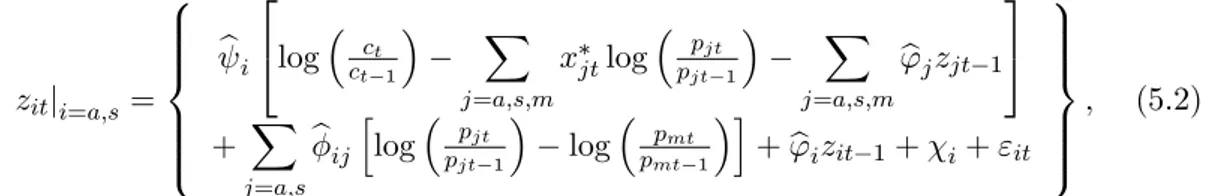
Given these constraints, one of the equations characterizing the Rotterdam model is redundant and, therefore, we should exclude it for the estimation.10 Since in our analysis we use three sectors (agriculture, manufactures and services), we eliminate the equation for the manufacturing sector. Furthermore, and after imposing the homogeneity constraint, we also obtain that the growth rates of consumption in agriculture and services depend on the growth rate of the relative prices of those goods in terms of manufactures, pat=pmt and pst=pmt: In this way, we derive the econometric speci…cation that we use to estimate income and Allen-Uzawa elasticities. Finally, we follow Brown and Lee (1992), who incorporate the e¤ect of past consumption to account for the possible existence of intertemporally-dependent preferences behind the observe demand because of, for instance, habit formation in consumption. With all of these features in hand, we obtain
zitji=a;s = 8 > > > > < > > > > : bi 2 4log ct ct 1 X j=a;s;m xjtlog pjtpjt 1 X j=a;s;m b 'jzjt 1 3 5 + X j=a;s bijhlog pjtpjt 1 log pmt pmt 1 i +'bizit 1+ i+ "it 9 > > > > = > > > > ; ; (5.2)
where i is a constant; zit = xitlog (cit=cit 1) ; xit = (xit 1+ xit) =2 is the average value of the share of good i in full income during the time increment being considered; and "it is the disturbance that we assume homoscedastic and uncorrelated over time. Furthermore, we also assume that this disturbance is normally distributed as N (0; ) ; where is the unknown contemporaneous covariance matrix.
We estimate (5.2) for the demand on agriculture and services goods by using the method of Seemingly Unrelated Regression Estimation since the disturbance vector " can be correlated across sectors. We further impose the symmetry constraint ij = ji: Note that we can skip the Engel aggregation constraint because we have omitted the equation for manufactures. On the contrary, the restriction on the Slutsky matrix has to be tested after the estimation.
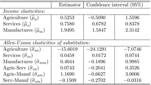
Table 1 displays the results of the estimation of the model (5.2). By using Engel aggregation and homogeneity constraints we can compute the corresponding coe¢ cients for the manufactures: bm = 0:439104, bam = 0:005606; bmm = 0:019488 and bms = 0:025094: The regression provides a quite good …t. All the marginal budget shares bi exhibit the expected positive sign, which means that the consumption goods are normal goods. Furthermore, all the coe¢ cients are estimated with considerable precision except ba and bas: Finally, we have checked that the Slutsky matrix ij is negative semide…ne and of rank m 1 = 2:
[Insert Table 1]
We now deduce the elasticity aggregates from our estimated coe¢ cients. To this end, we use the properties of the Rotterdam model which implies that the estimated income and Allen-Uzawa elasticities are given by bi = bi=xi and bij = bij= (xixj),
1 0
Barten (1969) proves that one equation of the demand system is redundant, and the maximum likelihood estimaties of the parameters are invariant to the equation deleted.
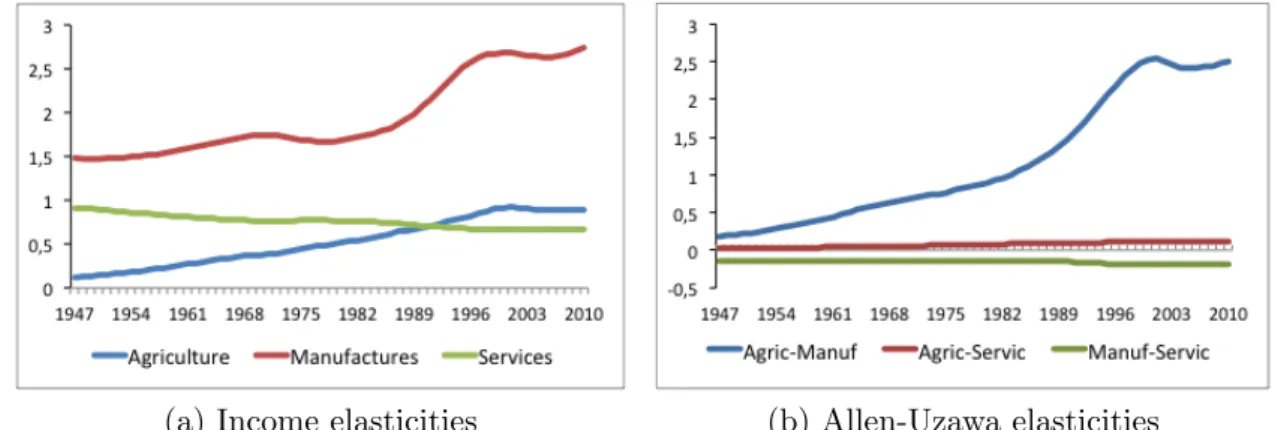
respectively. Obviously, these elasticities are varying. Figure 3 shows the time-path of these estimated elasticities and Table 2 displays their average values. Several properties should be pointed out. Firstly, with respect to income elasticities, we obtain that the three consumption goods are normal goods, although the estimation of the income elasticity of agriculture goods exhibits a large variability, such that its con…dence interval contains negative values. We observe that the demands of agriculture and services exhibits income elasticity smaller than unity, whereas the demand of manufactures exhibits an income elasticity larger than unity. The literature explaining structural change by means of non-homothetic preferences usually imposes a< m= 1 < sfor the calibration of the proposed models (see, e.g., Kongsamunt et al., 2001). The …rst inequality is corroborated by our estimations, whereas we obtain instead that ba < bs < 1 and bm > bs: We can explain the latter result by the fact that manufacturing sector produces durable goods and the service sector produces many basic goods for the consumption basket. Finally, Figure 3 shows thatba>bsat the end of the series, which may be a consequence of the change in the relative aspirations or necessities in consumption experimented by consumers along the development process.
[Insert Figure 3 and Table 2]
With respect to Allen-Uzawa elasticities, we …rst observe that bas 6= bam 6= bms; which means that composite consumption is not given by a standard CES aggregator of the consumption goods ca; cm and cs: Furthermore, we also conclude that agriculture goods are Hicks substitutes of manufactures and services as bam > 0 and bas > 0: However, the con…dence interval shows a large variability of these estimated elasticities, such that we can not reject these elasticities to be negative. Hence, we cannot reject that agriculture goods are Hicks complementaries or independent of manufactures and services. In addition, we also obtain bsm < 0; so that services and manufactures are Hicks complementaries.
5.2. Estimation of technological elasticities
The capital income shares i are directly taken from data. In addition, to estimate the elasticity of substitution, i; we consider that the cost functions are translog-functions and, thus, we derive the associate system of sectoral cost shares.11 Denote by Ti(Yi; r; w) the total cost of production in sector i. Because of constant returns to scale, it can be shown that Ti = Yi i(r; w); where i denotes the average cost function. By expanding ln i(r; w) in a second-order Taylor series about the point ln r = ln w = 0; by identifying the derivatives of the average cost function as coe¢ cients, and by imposing the symmetry of the cross-price derivatives, we obtain:
ln i = i0+ ikln ri+ illn wi+ 0:5 h i kk(ln ri)2+ ill(ln wi)2 i + iklln riln wi: This is the translog cost function. By taking derivatives with respect to ln ri and ln wi; we obtain that the cost shares of capital and labor in a sector i are respectively given by:
i = ik+ ikkln(ri) + iklln(wi); 1 1
and
1 i= il+ ilk ln(ri) + illln(wi); with the following conditions:
i k+ il = 1; i kl = ilk; and i kk+ ikl = ilk+ ill= 0:
By imposing these constraints, and taking the labor income shares 1 i directly from data, we then estimate the following system of equations:
it= ik ikkln (!it) + "it (5.3) for all i = fa; s; mg ; and where "itis the disturbance that we assume homoscedastic and uncorrelated over time. Furthermore, we also assume that this disturbance is normally distributed as N (0; ) ; where is the unknown contemporaneous covariance matrix. Since the disturbance vector " can be correlated across sectors, we estimate the system composed of the three equations (5.3) by using the method of Seemingly Unrelated Regression Estimation. Table 3 provides the estimates of the full set of parameters in (5.3). All the parameters are estimated with a large precision.
[Insert Table 3]
We now deduce sectoral elasticities of substitution between capital and labor i from our estimated coe¢ cients. Note that those are the elasticities of the marginal costs with respect to rental rates. Hence, we obtain:
bit= 1
bikk it(1 it)
:
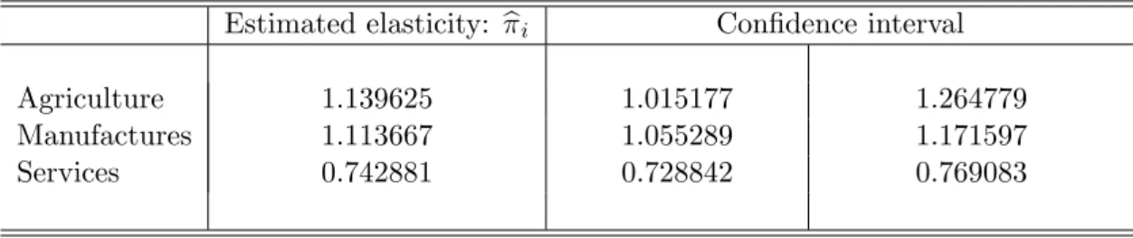
Observe that these elasticities are time-varying. Figure 4 shows the time-path of these estimated elasticities and Table 4 displays their average values. We can reject that bi = 1; i.e., Cobb-Douglas technologies at the sectoral level. More precisely, as was suggested, for instance, by Alvarez-Cuadradro et al. (2013), we obtain that capital and labor are complementary in services, whereas they are substitutes in manufactures and agriculture. These elasticities maintain these features along the entire dynamic path. In fact, these elasticities remains almost constant along the entire period.
[Insert Figure 4 and Table 4] 5.3. Accounting of mechanisms
The purpose of this subsection is to measure the importance of each mechanism. To this end, we develop the following experiment. We …rst compute the estimated sectoral employment shares and, furthermore, we measure how these estimates …t actual shares in the data. In addition, we build the counterfactual values of the sectoral employment shares that would arise if we turn o¤ one of the mechanisms of structural change in (3.7).
We then compute the change in the …t derived from this counterfactual experiment. More precisely, using the estimations in the previous subsections, we build the following counterfactual employment shares:
e
uit= eGituit 1;e for i = fa; s; mg and with
e
ui1= eGi1ui0;
where ui0 is the actual value of the US employment share in sector i at 1947; and Git is the growth factor in (3.7) that is de…ned as the sum of the following mechanisms of structural change:
The growth rate from the Real Income E¤ect:
GRIit =bi 2 4_c c X j=a;m;s xj _ pj pj 3 5 ;
The growth rate from the Demand Substitution E¤ect: GDSit = X j=a;m;s bijxj _ pj pj ;
The growth rate from the Technological Substitution E¤ect: GT Sit = ibi !_i
!i ;
The growth rate from the Technological Change E¤ect: GT Cit = ( ibi 1) i:
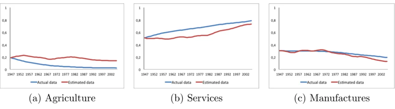
Figure 5 compares the path of the counterfactual employment shares feuig2005t=1948 with the one followed by actual shares fuig2005t=1948: We …rst observe that the …t of the counterfactual shares to the actual shares are not perfect. This is a consequence of two facts: (a) the luck of precision in the estimation of the elasticities; and, more importantly, (b) the omission of other possible mechanisms of structural change like, for instance, resource allocation to home production and leisure or international trade.
[Insert Figure 5]
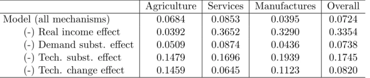
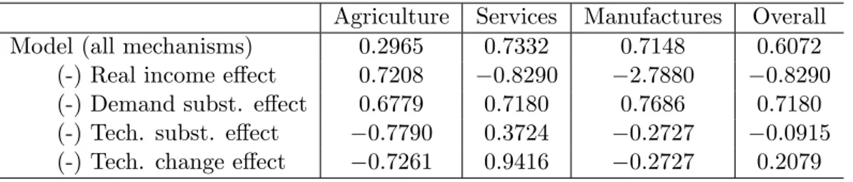
The goodness of …t is still very large as is con…rmed by the root mean-square error (RM SE) of the regression of the actual employment shares with respect to the counterfactual shares provided by Table 5. This table analyzes the performance of the simulation containing all mechanisms as well as the counterfactual simulations where one of the mechanism is turned o¤. Hence, their results provides an accounting exercise of the contribution of the di¤erent mechanisms for the entire sample period. We make this exercise for each sector, and we also provide the overall performance,
which is computed as a weighted average of the sectoral performance with the sectoral employment shares as the weights. Our simulations show that the technological change and the technological substitution e¤ects are the main mechanisms in explaining the evolution of the employment share in agriculture because the RM SE largely increases when one of these mechanisms are turned o¤, whereas the RM SE decreases when we switch o¤ the other two mechanism. By the contrary, the real income e¤ect is basically the main mechanism for the evolution of the employment share in services, although the technological substitution e¤ect has also a signi…cative e¤ect. Hence, as shown in the last column of the table, all mechanisms, with the exception of the demand substitution e¤ect, play a signi…cant role in explaining the structural change observed throughout the sample period.12 All of these mechanisms are then possible sources for the transmission of structural shocks like, for instance, …scal policy to the aggregate economy.
The results in Table 5 illustrate the existence of con‡icts among the mechanims in shaping the sectoral structure. In order words, the mechanims can operate in the opposite direction, so that the structural change results from the counterbalance among these forces. We speci…cally show what are the direction of the e¤ect from each mechanism by means of the Relocation Index (LRI) introduced by Swiecki (2013). The relocation index of labor in sector i measures the fraction of the change in labor share explained by the simulation. This measure is de…ned as
LRIi = 1
um
i udi udi ;
where umi = [um(tf) um(ti)] = (tf ti) measures the average annual change of labor share ui between years ti and tf according to the simulation and udi is the corresponding change in the share according to the data. If LRI = 1 the model explains the entire change in the variable and if LRI = 0 the model does not explain the change in the variable. Furthermore, this index takes negative values when the model predicts changes larger than twice the observed change or going in the opposite direction. Hence, this index is useful both for measuring the goodness of …t and for deriving which mechanims push on labor towards a sector and which ones pull on labor from this sector. Table 6 provides the values of this index for each of the sectors and counterfactual experiments. The index corroborates the conclusions derived from RM SE in Table 5 regarding both the simulations’performance and the accounting of the contribution of the mechanisms. We observe that the LRI always decreases when the RM SE increases.
[Insert Tables 5 and 6]
More interesting, we establish from the values of LRI in Table 6 the direction of the force that each mechanism exerts over labor in each sector. To this end, we do not have to focus only on the changes in the value of the index when we turn o¤ a mechanism, but also on the change in the sign of the index. If a mechanism operates in the same
1 2
Buera and Kabosky (2009) asserts that several mechanisms should be considered together to account for the entire set of facts on structural change.
direction as that of the observed dynamics, then the LRI index will either decrease or become negative when we turn it o¤. On the contrary, the index will increase when the excluded mechanism plays against the observed dynamics, as long as its impact is less than twice the net impact derived from the interaction between all the mechanisms. Hence, we conclude that the real income e¤ect and the demand substitution e¤ect largely push on labor towards agriculture and services, whereas the two technological e¤ects drive out labor of these sectors. However, the balance among mechanisms are the opposite in the two sectors. In spite that the real income and demand substitution e¤ects are isolately larger than the technological e¤ects in the agriculture, the latter e¤ects dominates because the balance among the e¤ects is …nally determined by the elasticities. The balance between mechanisms in the sector providing services is a little more complex. In this sector, the real income e¤ect is very large so that the LRI index become negative when we turn it o¤. The substitution e¤ect is extremely small, which explains the small reduction in the LRI index when this mechanism is omitted in the simulation. Even when the technological substitution e¤ect operates in the opposite direction of the one …nally followed by labor in services, the LRI index decreases when we turn o¤ this mechanism. This derived from the fact that the negative impact of this force is so large that the labor share would increase much more than we …nally observe if this mechanism will be not operative. By the contrary, the technological change e¤ect has a negative but small impact on the dynamics of labor in the services sector, so that the LRI index increases in the absence of this mechanism in the simulations. Obviously, the results in the manufacturing sector are a consequence of those obatined for agriculture and services as the labor dynamics in that sector is simulated as a residual from using the clearing condition in labor market: um= 1 ua us:
One advantage of our analysis is that we can decompose the observed patterns of structural change in two elements: (a) the contribution of the primary variation in prices, income and sectoral TFPs; and (b) the contribution of the changes in preferences and technologies, which are covered by the variation in demand and technological elasticities (i.e., i; ij; i and i): In order to measure the relative contribution of these two set of elements, we now repeat the previous analysis by taking the value of these elasticities at their respective cross-time average values (see Tables 2 and 4). In this way, we approximate the contribution of the variation in prices, income and sectoral TFPs to the observed structural change in the entire sample period. Of course, the contribution of the variation in the elasticities can be derived as a residual. Figure 6 and Tables 7 and 8 provide the …t of these new counterfactual simulations. The results on the relative contribution of the four derived mechanisms (i.e., real income, demand substitution, technological substitution and technological change e¤ects) still maintain when we consider time invariant elasticities. Furthermore, and more remarkly, the performance of our simulationsclearly worsens when the elasticities are taken constant. Therefore, assuming funtional forms for preferences and technologies that imply constant elasticities limits the ability of the models to explain the structural change.
[Insert Figure 6 and Tables 7 and 8]
Summarizing, we then conclude that the four mechanisms of structural change characterized in this paper have contributed substantially to the observed structural
change in US from 1947 to 2005. As was shown here, they generate con‡icting forces for sectoral structure because they have operated in the opposite direction. However, the observed structural change is the …nal result from the balance between these forces. Hence, any multisector growth model built to predict the e¤ects of structural shocks like, for instance, …scal policy should consider those mechanisms as fundamentals. Otherwise, one can derive biased results of those e¤ects.
6. Concluding Remarks
We have developed a theoretical and empirical analysis to identify all possible mechanisms driving the observed structural change and to disentangle the deep fundamentals of these factors. We have found that the following mechanisms have had a large e¤ect on the dynamics of sectoral employment shares: (i) the income e¤ects from the growth of income and from changes in relative prices; and (ii) the demand substitution and technological substitution e¤ects caused by the variation of prices derived from sectoral-biased technological progress, capital deepening and sectoral di¤erences in capital-labor substitution. The income e¤ect from the growth of income and the technological e¤ects have reallocated labor from agriculture to manufactures and services, whereas the demand substitution e¤ect and the income e¤ect, both derived from the variation in relative prices, have considerably restrained the previous movement of labor. Furthermore, we have shown that the economic fundamentals that are behind of structural change are: (i) the income elasticities of the demand for consumption goods; (ii) the Allen-Uzawa elasticities of substitution between consumption goods; (iii) the capital income shares in sectoral outputs; and (iv) the elasticity of substitution between capital and labor in each sector. These economic indicators determine the relative importance of the growth rates of aggregate income, relative prices, rental rates and technological progress for the structural change.
The research in this paper should be improved and extended in some directions. In the theoretical part, we should …rst include international trade, home production and leisure. On the one hand, we conjecture that an important fundamental driving the e¤ect of international trade would be the elasticities of demand for imported goods and the Allen-Uzawa elasticities of substitution between domestic and foreign consumption goods. In this sense, the analysis should not be very di¤erent to that developed in this paper after having incorporated foreign consumption good to the composite good from which individuals derive utility. On the other hand, in the case of leisure and home production, one would expect that the complementarity between goods and services would be crucial for the structural change as was pointed out by Cruz and Raurich (2015). Secondly, the theoretical analysis should be also extended to derive the conditions that makes structural change, jointly driven by all of the considered mechanisms, compatible with the existence of balanced growth of aggregate variables as the data suggest.
The empirical part of our analysis might be modi…ed in the following points. First, we might also estimate the demand elasticities by using a more ‡exible functional form for the indirect utility function. In other words, we might confront whether or not the estimation of a translog indirect utility function is more precise than the estimation of the Rotterdam model considered in the paper. Second, we might try to improve
the estimation procedure by considering other methods and by extending the length of the period. Finally, we might perform a cross-country analysis conditioned on the availability of data.
In addition to the previous extensions, we might also postulate a dynamic general equilibrium model that includes all the mechanisms of structural change. We should calibrate this model by using our estimations of the fundamentals behind these mechanisms. This would …rst allow us to study numerically how is the …t of the observed structural change. We then can use this model to develop experiments to assess the e¤ects of …scal policy and public regulations on sectoral and aggregate variables.
References
[1] Acemoglu, D. and Guerrieri, V. (2008). Capital deepening and non-balanced economic growth. Journal of Political Economy 116, 467-498.
[2] Alonso-Carrera, J. and Raurich, X. (2016). Labor mobility, structural change and economic growth. UBEconomics Working Papers E15/325.
[3] Alvarez-Cuadrado, F., Van Long, N. and Poschke, M. (2013). Capital Labor Substitution, Structural Change and Growth. Manuscript, McGill University, Montreal.
[4] Barnett, W.A. (1981). Consumer demand and labor supply. Amsterdam: North-Holland Publishing Company.
[5] Barten, A.P. (1964). Consumer Demand Functions Under Conditions of Almost Additive Preferences. Econometrica 32, 1-38.
[6] Barten, A.P. (1969). Maximum Likelihood Estimation of Complete System of Demand Equations. European Economic Review 1, 7-73.
[7] Baumol, W. (1967). Macroeconomics of unbalanced growth: the anatomy of urban crisis. American Economic Review 57, 415-426.
[8] Brown, M.C. and Lee, J.Y. (1992). Adynamic di¤erential demand system: an application of translation. Southem Journal of Agricultural Economics 24, 1-10. [9] Buera, F. and Kaboski, J. (2009). Can traditional theories of structural change …t
the data? Journal of the European Economic Association 7, 469-477.
[10] Caselli, F., Coleman, J.W. II. (2001). The U.S. structural transformation and regional convergence: A reinterpretation. Journal of Political Economy 109, 584-616.
[11] Comin, D., Lashkari, D., Mestieri, M. (2015). Structural change with long-run income and price e¤ects. NBER Working Papers 21595.
[12] Cruz, E., Raurich, R. (2015). Leisure time and the sectoral compostion of employment. Manuscript.
[13] Deaton, A. (1983). Demand analysis. Handbook of Econometrics, Z. Griliches and M. Intriligator (eds.). Amsterdam: North-Holland Publishing Company.
[14] Deaton, A., Muellbauer, J. (1980). Economics and consumer behavior. New York: Cambridge University Press.
[15] Dennis, B.N., Iscan, T.B. (2009). Engel versus Baumol: Accounting for structural change using two centuries of U.S. data. Explorations in Economic History 46, 186-202.