Institut de Recerca en Economia Aplicada Regional i Pública Document de Treball 2018/06 1/26 pág. Research Institute of Applied Economics Working Paper 2018/06 1/26 pág.
“A geometric approach to proxy economic uncertainty by a
metric of disagreement among qualitative expectations
”
4
WEBSITE: www.ub.edu/irea/ • CONTACT: [email protected]
The Research Institute of Applied Economics (IREA) in Barcelona was founded in 2005, as a research institute in applied economics. Three consolidated research groups make up the institute: AQR, RISK and GiM, and a large number of members are involved in the Institute. IREA focuses on four priority lines of investigation: (i) the quantitative study of regional and urban economic activity and analysis of regional and local economic policies, (ii) study of public economic activity in markets, particularly in the fields of empirical evaluation of privatization, the regulation and competition in the markets of public services using state of industrial economy, (iii) risk analysis in finance and insurance, and (iv) the development of micro and macro econometrics applied for the analysis of economic activity, particularly for quantitative evaluation of public policies.
IREA Working Papers often represent preliminary work and are circulated to encourage discussion. Citation of such a paper should account for its provisional character. For that reason, IREA Working Papers may not be reproduced or distributed without the written consent of the author. A revised version may be available directly from the author.
Any opinions expressed here are those of the author(s) and not those of IREA. Research published in this series may include views on policy, but the institute itself takes no institutional policy positions.
Abstract
In this study we present a geometric approach to proxy economic uncertainty. We design a positional indicator of disagreement among survey-based agents' expectations about the state of the economy. Previous dispersion-based uncertainty indicators derived from business and consumer surveys exclusively make use of the two extreme pieces of information coming from the respondents expecting a variable to rise and to fall. With the aim of also incorporating the information coming from the share of respondents expecting a variable to remain constant, we propose a geometrical framework and use a barycentric coordinate system to generate a measure of disagreement, referred to as a discrepancy indicator. We assess its performance, both empirically and experimentally, by comparing it to the standard deviation of the share of positive and negative responses, which has been used by Bachman et al. (2013) as a proxy for economic uncertainty. When applied in sixteen European countries, we find that both time-varying metrics co-evolve in most countries for expectations about the country's overall economic situation in the present, but not in the future. Additionally, we obtain their simulated sampling distributions and we find that the proposed indicator gravitates uniformly towards the three vertices of the simplex representing the three answering categories, as opposed to the standard deviation, which tends to overestimate the level of uncertainty as a result of ignoring the no-change responses. Consequently, we find evidence that the information coming from agents expecting a variable to remain constant has an effect on the measurement of disagreement.
JEL Classification: C51, C55, C63, C83, C93.
Keywords:Economic uncertainty, disagreement, expectations, economic tendency surveys, geometry, barycentric coordinate system, spatial vectors. Oscar Claveria AQR-IREA, University of Barcelona (UB). Tel.: +34-934021825; Fax.: +34-934021821. Department of Econometrics, Statistics and Applied Economics, University of Barcelona, Diagonal 690, 08034 Barcelona, Spain. E-mail address:
Enric Monte. Department of Signal Theory and Communications, Polytechnic University of Catalunya (UPC)
Salvador Torra. Riskcenter-IREA, Department of Econometrics and Statistics, University of Barcelona (UB)
Acknowledgements
This research was supported by by the projects ECO2016-75805-R and TEC2015-69266-P from the Spanish Ministry of Economy and Competitiveness. We also wish to thank Anna Stangl, Johanna Garnitz and Klaus Wohlrabe at the Ifo Institute for Economic Research in Munich for providing us the data used in the study.
1. Introduction
The arrival of the 2008 financial crisis has triggered a body of research dedicated to analyse the impact of uncertainty on the economy (Ajmi et al., 2015; Arslan et al., 2015; Atalla et al., 2016; Balcilar et al., 2017; Binder, 2017; Binding and Dibiasi, 2017; Bloom, 2014; Caggiano et al., 2014; Chua et al., 2011; Dovern, 2015; Fernández-Villaverde et al., 2015; Hartmann et al., 2017; Henzel and Rengel, 2017; Karnizova and Li, 2014; Mitchell et al., 2017; Mokinski et al., 2015; Perić and Sorić, 2017; Sorić and Lolić, 2017). Since economic uncertainty is not directly observable, several strategies have been proposed to measure it.
A first approach consists on tracking the magnitude of forecast errors of macroeconomic variables (Glass and Fritsche, 2014; Jurado et al., 2015). This approach is based on the assumption that in times of high uncertainty forecast errors are expected to rise, but its ex-post nature has led researchers to develop alternative approaches to measure economic uncertainty.
A second approach is based on the assumption that notions about the future evolution of the economy are likely to be more disperse in times of high uncertainty. This premise allows to develop dispersion-based indicators. These measures can either be based on stock market volatility (Basu and Bundick, 2012; Bekaert et al., 2013; Bloom, 2009), or on agents’ economic expectations (Glas and Hartmann, 2016; Lahiri and Sheng, 2010; Mankiw et al., 2004; Mokinski et al., 2015).
Direct measures of expectations can only be derived from surveys. Tendency surveys ask respondents whether they expect a variable to rise, fall or remain unchanged. By using agents’ expectations coming from economic tendency surveys, Bachman et al. (2013) proposed a set of uncertainty indicators based on the dispersion of respondents’ expectations about the future in Germany and the United States (US). Girardi and Reuter (2017) have recently presented three new dispersion-based uncertainty indicators derived from business and consumer surveys for the Euro Area (EA).
All these dispersion-based indicators of disagreement among respondents elicit the information exclusively form the respondents expecting a variable to rise and to fall, leaving out the the responses from agents expecting no-change. This omission has led us to devise an approach that allows to derive a time-varying disagreement metric that incorporates the information coming from all three answering categories.
2
With this aim, we present a geometric setup to construct a positional indicator of disagreement that can be interpreted as the percentage of discrepancy among responses. We focus on agents’ expectations about the country’s situation regarding the overall economy both at present and by the end of the next six months. We compare the performance of the proposed measure of displacement to the standard deviation of the share of positive and negative responses, which has been used by Bachman et al. (2013) as a proxy for economic uncertainty. The analysis is carried out in sixteen European countries, focusing on the period prior to the start of the 2008 financial crisis, which provides a natural backdrop for the experiment. Finally, we simulate the sampling distribution of both indicators to further assess their performance.
The structure of the paper is as follows. The next section introduces the data. In Section 3 we present the methodological approach. Empirical results are provided in Section 4. Finally, concluding remarks and future lines of research are drawn in Section 5.
2. Survey data on expectations
Uncertainty is unobservable. Economic uncertainty can be defined as the situation in which economic agents are not able to anticipate future events or estimate the likelihood of their occurrence (Knight, 1921). Since the advent of the 2008 financial crisis, there has been a renewed interest in the measurement of economic uncertainty. Baker et al. (2016) designed the economic policy uncertainty (EPU) index, which is based on three components: a media index of economic uncertainty, the number of federal expiring tax code provisions and a disagreement measure based on the responses from the Surveys of Professional Forecasters.
While the development of machine learning techniques increasingly facilitates the generation of ad-hoc media indexes of frequencies of keyword combinations related to uncertainty that avoid the pre-labelling of the data (Azqueta-Gavaldón, 2017), this approach still entails a non-negligible degree of subjectivity (Girardi and Reuter, 2017). As a result, based on the assumption that the dispersion of expectations increases during periods of high uncertainty, one of the most common approaches to proxy economic uncertainty is to use measures of disagreement among survey expectations (Giordani and Söderlind 2003; Glass and Hartmann, 2016; Lahiri and Sheng, 2010; Mokinski et al., 2015; Rich and Tracy 2010; Zarnowitz and Lambros 1987).
Economic expectations are not directly observable, and therefore are elicited through survey data. Recent research has shown that the data provided by business and consumer tendency surveys is particularly useful in order to derive uncertainty measures based on the dispersion of expectations (Bachmann et al., 2013; Mokinski et al., 2015). Bachmann et al. (2013) found that during times of high uncertainty respondents tend to give more heterogeneous answers to the questions focused on relevant economic variables. As a result, the authors approximated uncertainty by the degree of disagreement among economic forecasters by means of three alternative proxies. In a recent research, Girardi and Reuter (2017) have proposed three new dispersion-based uncertainty indicators derived from economic tendency surveys.
These measures are based on the responses that fall into the two extreme answering categories, that is, the respondents expecting a variable to increase and the ones expecting it to decrease. In this study, we want to evaluate the effect of incorporating the information coming from the respondents expecting a variable to remain constant.
With this aim we use raw data from the World Economic Survey (WES) carried out quarterly by the Ifo Institute for Economic Research. The WES assesses worldwide economic trends by polling professionals and experts on current economic developments in their respective countries. We focus on the question about the country’s situation in terms of its overall economy, both present and future. We use the shares of respondents expecting a variable to go up, to go down or to remain unchanged during the period ranging from 2005:Q2 to 2008:Q4. This time frame allows us to capture the evolution of expectations prior to a significant impending shock in sixteen European countries countries (Austria, Belgium, Finland, France, Germany, Greece, Hungary, Italy, Latvia, the Netherlands, Poland, Portugal, Romania, Spain, Sweden and the United Kingdom).
In Fig. 1 we compare the evolution of no-change expectations (percentage respondents expecting their country’s economic situation to remain constant) to the year-on-year GDP growth rates. We use quarterly GDP data from the OECD (https://data.oecd.org/gdp/quarterly-gdp.htm#indicator-chart). Overall, it can be seen that in most countries the proportion of no-change responses remains low and fairly constant up until 2007, when it significantly rises as the economic activity starts to fall. As a result, it seems that the share of no-change responses behaves counter-cyclically, suddenly increasing during periods of high uncertainty.
4 Fig. 1a. Evolution of year-on-year GDP growth rates vs. share of no-change responses
Austria Belgium
Finland France
Germany Greece
Hungary Italy
1. Note: The grey dotted line represents the evolution of the percentage of no-change responses regarding the current assessment of the country’s current situation in terms of its overall economy, while the black line the percentage regarding the expected assessment by the end of the next 6 months. The black dotted line represents the year-on-year growth rate of GDP in each country (secondary axis).
Fig. 1b. Evolution of year-on-year GDP growth rates vs. share of no-change responses
Latvia Netherlands
Poland Portugal
Romania Spain
Sweden United Kingdom
6 Table 1. Share of ‘no-change’ responses – Summary statistics (2005:Q2-2008:Q4)
No-change expectations Mean proportion Standard deviation Correlation with GDP Austria Present 0.043 0.072 -0.570* Future 0.272 0.265 -0.752** Belgium Present 0.139 0.229 -0.948** Future 0.303 0.261 -0.562* Finland Present 0.003 0.011 -0.013 Future 0.212 0.221 -0.857** France Present 0.282 0.232 -0.710** Future 0.214 0.187 -0.812** Germany Present 0.167 0.237 -0.486 Future 0.243 0.231 -0.667** Greece Present 0.110 0.057 -0.755** Future 0.252 0.228 -0.647** Hungary Present 0.312 0.116 -0.269 Future 0.284 0.157 -0.185 Italy Present 0.507 0.315 -0.444 Future 0.189 0.154 -0.645** Latvia Present 0.052 0.094 -0.917** Future 0.293 0.291 -0.760** Netherlands Present 0.153 0.245 -0.206 Future 0.223 0.291 -0.822** Poland Present 0.012 0.022 0.020 Future 0.217 0.247 -0.758** Portugal Present 0.613 0.203 -0.491 Future 0.077 0.155 -0.817** Romania Present 0.100 0.080 0.523* Future 0.137 0.194 -0.704** Spain Present 0.155 0.285 -0.962** Future 0.381 0.243 -0.816** Sweden Present 0.037 0.080 -0.831** Future 0.237 0.225 -0.895** UK Present 0.132 0.228 -0.834** Future 0.366 0.251 -0.725**
Notes: * Correlation is significant at the 0.05 level (2-tailed). ** Correlation is significant at the 0.01 level (2-tailed).
In Table 1 we present the summary statistics for the proportion of no-change responses. Results corroborate the counter-cyclical behaviour observed in Fig. 1. In most countries we obtain a negative and significant correlation between the evolution of no-change responses and GDP growth. This inverse relation has led us to devise a geometric approach to derive a time-varying uncertainty proxy based on disagreement among respondents that allows incorporating the information coming from all three answering categories. Geometry has previously been used to determine the likelihood of disagreement among election outcomes (Saari, 2008), but never before in this context.
3. Methodology
In this section we present a geometric approach to derive a dispersion-based measure of positional disagreement. The proposed framework allows to capture the proportion of discrepancy among survey respondents in any given period by means of spatial vectors. Tendency surveys are addressed to economic agents in order to elicit subjective measures of their expectations about the state of the economy. Respondents are asked about the expected direction of change of a wide range of variables (inflation, consumption, etc.). In this study we focus on the expectations about the country’s situation in terms of its overall economy, both at present and by end of the next six months.
Survey results are available about one quarter ahead of the publication of quantitative official data and are usually presented as balances, 𝐵𝑡 , which consist on the subtraction
between the weighted percentage of respondents expecting a variable to go up (𝑅𝑡) and to go down (𝐹𝑡). Nevertheless, survey results can be aggregated in a three dimensional
vector denoted as 𝑉𝑡:
𝑉𝑡= (𝑅𝑡, 𝐸𝑡, 𝐹𝑡) (1)
where 𝐸𝑡 refers to the proportion of respondents expecting the variable to remain constant.
The variance of the balance could be defined as:
𝐷𝑡 = 𝑅𝑡+ 𝐹𝑡− 𝐵𝑡2 (2)
Theil (1955) defined expression (2) as the disconformity coefficient, due to the fact that the value of 𝐷𝑡 would reach the minimum value zero when all the responses are concentrated in either one of the two categories. The maximum disconformity, corresponding to a value of one, would take place, if and only if, 𝑅𝑡 and 𝐹𝑡 each accumulates half of the responses. Expression (2) implicitly neglects the variate 𝐸𝑡. As a
result, the ‘no-change’ proportion is not directly incorporated into the disagreement metric. Claveria (2010) proposed a nonlinear variation of the balance statistic that accounted for this percentage of respondents.
Bachmann et al. (2013) used an economic uncertainty proxy denoted as 𝐷𝐼𝑆𝑃𝑡 that can be defined as the square root of 𝐷 at time t:
8
The authors applied this measure to the forward-looking survey question related to the expectations of domestic production activities in Germany at the micro level. Girardi et al. (2017) developed an aggregate variation of expression (3) in order to compute the cross-sectional standard deviation of the share of positive and negative responses for all forward-looking survey questions, and then standardised the question-specific measures and rescaled the average dispersion.
With the aim of incorporating the information coming from the respondents expecting no-change in the variable, we develop a methodological framework that allows to construct a measure of disagreement that conveys a geometrical interpretation. The proposed metric presents two inherent advantages. On the one hand, it allows to capture the trajectories of the three states. On the other hand, it has a self-explanatory interpretation, as it provides the proportion of disagreement among respondents.
In order to explicitly incorporate the three components of the surveys (𝑅𝑡, 𝐸𝑡, 𝐹𝑡), we
assume that no-change responses can proxy either one of the extreme options. Note that the fraction of answers falling into the ‘no-change’ category is conveying the information about the confidence on the other two categories. Kahneman (2011) noted that when faced with a difficult question, respondents often choose an easier one instead.
As the sum of the proportions adds to a constant, a natural representation of the answers will be as a point on a simplex (Coxeter, 1969). A simplex could be defined as the smallest convex set containing the given vertices. We will use a two-dimensional simplex, which corresponds to a triangle. The interior of this simplex encompasses all possible combinations of proportions between the three answering categories.
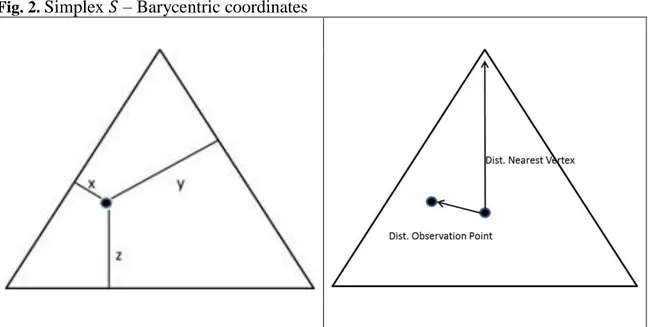
The equilateral triangle 𝑆 can be defined by its three vertices {x, y, z} (see left panel of Fig. 2). A simplex in ℝ3 can be defined as 𝑎
1𝑥 + 𝑎2𝑦 + 𝑎3𝑧 , such that 𝑎1+ 𝑎2+
𝑎3 = 1 and 𝑎1, 𝑎2, 𝑎3 ≥ 0, where 𝑎1, 𝑎2 and 𝑎3 stand for the three proportions defined in (1). These proportions can be regarded as the barycentric coordinates of a point with respect to 𝑆. Therefore, each point inside 𝑆 has a unique convex combination of the three vertices determined by the set of aggregated survey results.
The barycentric coordinate system allows us to compute the vertical distance of a point in the simplex to the nearest edge, as it can be seen in the right panel of Fig. 2. As there are two degrees of freedom, any set of barycentric coordinates and their corresponding basis vectors can be used to define the location of any point within 𝑆.
Fig. 2. Simplex 𝑆 – Barycentric coordinates
Once we have defined the location of the point within the simplex, we formalise a measure of consensus. We aim to define a measure that summarises the notion that if the coordinate on the simplex is near a vertex, there is a general agreement in the survey about that particular result. Conversely, if the coordinate is near the barycentre, which is the point of equal barycentric coordinates, one would expect little agreement on the opinions among the respondents. Thus, the center of the simplex indicates the point of maximum discrepancy among respondents. We can then compute a metric of consensus as a ratio on the simplex as follows:
Concentration = Distance of the observation point to the barycentreDistance of a vertex to the barycentre (4) Given that all vertices are at the same distance to the barycentre, this ratio gives the relative weight of the distance of each point in time to the center of the triangle. We can then formalise concentration for period 𝑡 as 𝐶𝑡 as:
C
t=
√(Rt-1/3)2+(Et-1/3)2+(Ft-1/3)2√2 3⁄ (5)
Consequently, the proposed geometry-based disagreement measure, which will be referred to as a discrepancy indicator, can be defined as the inverse of consensus:
10 4. Empirical results
In this section we apply the methodology presented in the previous section to sixteen European countries. First, we project survey answers in the simplex for each period of the sample (2005:Q2-2008:Q4). As an example, in Fig. 3 we show the projections for the last three quarters of the sample prior to the crisis, both for the expectations about the current situation and the one expected by the end of the next six months in Germany. As it can be seen, each point in the simplex takes into account the proportion of each of the three answering categories.
Fig. 3. Barycentric coordinates (2008:Q2–2008:Q4) – Germany
Expectations about the country’s current situation regarding overall economy
2008:Q2 2008:Q3 2008:Q4
Expectations about the country’s situation regarding overall economy for the next 6 months
2008:Q2 2008:Q2 2008:Q2
Second, by means of the barycentric coordinates of each point we compute 𝐺𝑡. To assess the performance of this metric of positional discrepancy we compare it to the uncertainty proxy proposed by Bachmann et al. (2013) defined in (3). Both indicators are bounded between zero and one. A one value indicates maximum disagreement, while zero maximum consensus. Additionally, we compute the expectational forecast errors by transforming survey indicators of the WES into quantitative estimates of economic growth using the coincident and the leading conversion indicators suggested by Claveria et al. (2017).
Fig. 4a. Evolution of disagreement measures and expectational forecast errors – Present Austria Belgium Finland France Germany Greece Hungary Italy
3. Note: The black solid line represents the evolution of the proposed indicator of discrepancy. The grey dotted line represents the evolution of Bachmann et al.’s (2013) disagreement indicator for the expectations about the present economic situation. The black dotted line represents the standardised expectational forecast errors (secondary axis).
12 Fig. 4b. Evolution of disagreement measures and expectational forecast errors – Present
Latvia Netherlands
Poland Portugal
Romania Spain
Sweden United Kingdom
Fig. 5a. Evolution of disagreement measures and expectational forecast errors – Future
Austria Belgium
Finland France
Germany Greece
Hungary Italy
5. Note: The black solid line represents the evolution of the proposed indicator of discrepancy. The grey dotted line represents the evolution of Bachmann et al.’s (2013) disagreement indicator for the expectations about the future economic situation. The black dotted line represents the standardised expectational forecast errors for future expectations (secondary axis).
14 Fig. 5b. Evolution of disagreement measures and expectational forecast errors – Future
Latvia Netherlands
Poland Portugal
Romania Spain
Sweden United Kingdom
Table 2. Summary statistics for measures of disagreement
𝐺𝑡 𝐷𝐼𝑆𝑃𝑡
Present Mean Standard
Deviation Mean Standard Deviation Correlation Austria 0.41 0.07 0.87 0.11 0.338 Belgium 0.41 0.11 0.77 0.21 0.571* Finland 0.24 0.19 0.65 0.30 0.948** France 0.37 0.13 0.55 0.16 0.375 Germany 0.44 0.09 0.78 0.17 0.044 Greece 0.38 0.13 0.70 0.17 0.849** Hungary 0.48 0.11 0.59 0.10 0.509 Italy 0.35 0.13 0.50 0.13 0.569* Latvia 0.39 0.15 0.77 0.30 0.860** Netherlands 0.37 0.13 0.70 0.25 0.538* Poland 0.45 0.04 0.94 0.04 0.645** Portugal 0.39 0.12 0.46 0.08 0.966** Romania 0.55 0.15 0.89 0.06 0.112 Spain 0.43 0.10 0.82 0.21 0.840** Sweden 0.34 0.22 0.73 0.26 0.711** UK 0.41 0.17 0.73 0.30 0.844** Future Mean Std. Deviation Mean Std. Deviation Austria 0.46 0.12 0.71 0.19 0.438 Belgium 0.50 0.13 0.71 0.18 0.404 Finland 0.53 0.11 0.79 0.16 0.261 France 0.57 0.12 0.79 0.17 0.095 Germany 0.55 0.13 0.79 0.14 -0.004 Greece 0.39 0.15 0.60 0.18 0.572* Hungary 0.65 0.14 0.77 0.10 0.388 Italy 0.59 0.09 0.83 0.13 -0.264 Latvia 0.44 0.22 0.63 0.25 0.528* Netherlands 0.43 0.19 0.74 0.17 0.294 Poland 0.54 0.11 0.82 0.16 0.175 Portugal 0.41 0.09 0.84 0.14 0.337 Romania 0.50 0.12 0.83 0.16 0.225 Spain 0.42 0.08 0.57 0.08 0.462 Sweden 0.45 0.13 0.69 0.19 -0.262 UK 0.44 0.11 0.61 0.12 0.285
Notes: Both indicators are bounded between zero and one. A one value indicates maximum disagreement; while zero, maximum consensus. * Correlation is significant at the 0.05 level (2-tailed). ** Correlation is significant at the 0.01 level (2-(2-tailed).
16
In Table 2 we present the mean and the standard deviation displayed by both dispersion-based disagreement measures. The fact that the proposed positional metric takes into account the share of no-change responses leads to lower mean values of disagreement in all countries. In Fig. 4 we can see that 𝐺𝑡 and the disagreement indicator
proposed by Bachmann et al. (2013) applied to the expectations of the country’s overall economic situation co-evolve for the present, but not so much for the future (Table 2).
With the aim of further assessing the performance of both indicators, we sample the simplex defined in section 3. We generate a uniform set of points in the unit cube, and then normalise each point such that the sum of the coordinates is equal to one. This procedure is equivalent to projecting the distribution onto a plane in order to sample the simplex of both metrics of disagreement among respondents.
In Fig. 6 we depict the overlapped non-normalised histograms of both statistics. While both distributions are similar and negatively skewed, the positional discrepancy indicator proposed in this study shows a fatter tail, suggesting a higher level of granularity. In Table 3 we present the summary statistics of both simulated distributions. We complement them with the boxplots (Fig. 7), which represent the distribution through their quartiles without making any assumptions of the underlying statistical distribution. The interquartile range (IQR) is a measure of statistical dispersion obtained as the difference between upper and lower quartiles, Q3−Q1.
As shown in Fig. 7, the distribution of the discrepancy indicator encompasses a much wider range of the scale, and the distribution of scores is more uniform. The IQR in Table 4 differs between both distributions, being significantly larger for 𝐺𝑡. This result is indicative of a higher level of granularity for the median values of the distribution of the discrepancy indicator in comparison to Bachmann et al.’s (2013) disagreement indicator. In Fig. 8 we project the barycentric coordinates of the simulated points in the simplex for both indicators. We complement the graphs with a comparative histogram representing the percentage of area in each decile. The higher granularity of the indicator proposed in this article is manifested by the fact that the areas for each level of scores is more uniform, which also can be seen in the decile distribution. We can see that the proposed geometric indicator of discrepancy behaves uniformly in all three directions, while the disconformity indicator shows a wider area in which gives a maximum value of disagreement. This result is caused by not taking into account the share of no-change responses.
Fig. 6. Histogram of simulated distribution – 𝐷𝐼𝑆𝑃𝑡 vs. 𝐺𝑡
Note: The lighter histogram represents the distribution of the proposed positional indicator of discrepancy; while the darker histogram at the back represents the distribution of the disagreement measure proposed by Bachmann et al. (2013). Both indicators are bounded between zero and one. A one value indicates maximum disagreement; while zero, maximum consensus.
Table 4. Summary statistics of simulated distribution of disagreement measures
Mean Std. Dev. Min. Max. Range IQR
𝐷𝐼𝑆𝑃𝑡 0.742 0.137 0.054 1.000 0.946 0.195
𝐺𝑡 0.662 0.176 0.004 0.998 0.994 0.255
Note: The Range is obtained as the difference between the maximum and the minimum values of the distribution. The IQR refers to the interquartile range, which is obtained as the difference between upper and lower quartiles, Q3−Q1.
Fig. 7. Boxplots of simulated distributions – 𝐷𝐼𝑆𝑃𝑡 vs. 𝐺𝑡
𝐷𝐼𝑆𝑃𝑡 𝐺𝑡
Note: The boxplot to the left represents the distribution of the disagreement measure proposed by Bachmann et al. (2013), while the one to the right that of the proposed positional indicator of discrepancy. A one value indicates maximum disagreement; while zero, maximum consensus.
18 Fig. 8. Projection of barycentric coordinates of simulated points onto the simplex
𝐷𝐼𝑆𝑃𝑡 𝐺𝑡
Note: In the upper panel, the simplex to the left represents the distribution of the disagreement measure proposed by Bachmann et al. (2013), while the one to the right that of the proposed positional indicator of discrepancy. A one value indicates maximum disagreement; while zero, maximum consensus. In the lower panel, we represent the percentage of area in each decile. The darker bars represent the distribution of the proposed positional indicator of discrepancy.
5. Concluding remarks
This paper presents a geometrical framework to proxy economic uncertainty by means of a survey-based measure of disagreement among respondents. The fact that tendency surveys ask agents whether they expect a particular variable to increase, decrease or remain unchanged, has lead us to design an indicator that takes into account all three magnitudes. Previous dispersion-based uncertainty indicators derived from business and consumer surveys exclusively make use of the two extreme pieces of information, that is, the responses expecting a variable to rise and to fall.
Our main aim was to incorporate the share of respondents expecting a variable to remain constant. With this objective, we project survey responses onto a simplex that takes the form of an equilateral triangle, and by means of spatial vectors we derive a measure of displacement that incorporates all three pieces of information.
To assess the performance of the proposed measure of positional discrepancy we compare it, both empirically and experimentally, to the standard deviation of the share of positive and negative responses, which has been used by Bachman et al. (2013) as a measure of disagreement. First, we compute both measures for sixteen European countries, finding that they co-evolve during the sample period in most countries, especially for the expectations about the country’s current economic situation.
Second, we generate the simulated sampling distributions of both the proposed geometric indicator of discrepancy and the disagreement measure used as a benchmark. In spite of the fact that both distributions are negatively skewed and similar, we find that the distribution of the proposed positional indicator of discrepancy shows a fatter tail, suggesting a higher level of granularity for the intermediate values, which is confirmed by a higher value of the interquartile range.
By projecting the barycentric coordinates of the simulated points onto the simplex, we observe that the proposed discrepancy indicator gravitates uniformly towards the three vertices of the triangle, defined by the three answering categories. Conversely, the disagreement measure used as a benchmark tends to overestimate the level of uncertainty as a result of ignoring the no-change share of responses. Arguably, it seems that the information coming from agents expecting a variable to remain constant has an effect on the measurement of disagreement among survey respondents.
20
In spite of the novelty of the approach, the metric presented in the paper is not without limitations. The proposed geometrically-based discrepancy indicator is a measure of disagreement among survey respondents, and as such has to be considered a proxy of uncertainty, which is a latent variable. As noted by Girardi et al. (2017), the evolvement of survey-based disagreement indicators does not only reflect changes in underlying uncertainty levels, but also in heterogeneity among agents’ expectations. An issue left for further research is extending the construction of the indicator on the basis of responses to additional variables. Another line of future research is the analysis of the impact of the proposed uncertainty metric on economic activity.
References
Ajmi, A. N., Aye, G. C., Balcilar, M., and El Montasser, G. (2015). Casualty between US economic policy and equity market uncertainties: Evidence form linear and nonlinear tests. Journal of Applied Economics, 18(2), 225–246.
Arslan, Y., Atabek, A., Hulagu, T., and Şahinöz, S. (2015). Expectation errors, uncertainty, and economic activity. Oxford Economic Papers, 67(3), 634–660.
Atalla, T., Joutz, F., and Pierru, A. (2016). Does disagreement among oil price forecasters reflect volatility? Evidence form the ECB surveys. International Journal of Forecasting, 32(4), 1178–1192.
Azqueta-Gavaldón, A. (2017). Developing news-based economic policy uncertainty index with unsupervised machine learning. Economics Letters, 158, 47–50.
Bachmann, R., Elstner, S., and Sims, E. R. (2013). Uncertainty and economic activity: Evidence from business survey data. American Economic Journal: Macroeconomics, 5(2), 217– 249.
Baker, S. R., Bloom, N., and Davis, S. J. (2016). Measuring economic policy uncertainty.
Quarterly Journal of Economics, 131(4), 1593–1636.
Balcilar, M., Bekiros, S., and Gupta, R. (2017). The role of news-based uncertainty indices in predicting oil markets: a hybrid nonparametric quantile causality method. Empirical
Economics, 53(3), 879–889.
Basu, S, and Bundick, B. (2017). Uncertainty shocks in a model of effective demand.
Econometrica, 85(3), 937–958.
Bekaert, G., Hoerova, M., and Lo Duca, M. (2013). Risk, uncertainty and monetary policy.
Journal of Monetary Economics, 60(7), 771–788.
Binder, C. (2017). Measuring uncertainty based on rounding: New method and application to inflation expectations. Journal of Monetary Economics, 90, 1–12.
Binding, G., and Dibiasi, A. (2017). Exchange rate uncertainty and firm investment plans evidence from Swiss survey data. Journal of Macroeconomics, 51, 1–27.
Bloom, N. (2009). The impact of uncertainty shocks. Econometrica, 77(3), 623–685.
Bloom, N. (2014). Fluctuations in uncertainty. Journal of Economic Perspectives, 28(2), 153– 176.
Caggiano, G., Castelnuovo, E., and Groshenny, N. (2014). Uncertainty shocks and
unemployment dynamics in U.S. recessions. Journal of Monetary Economics, 67(C), 78– 92.
Claveria, O. (2010). Qualitative survey data on expectations. Is there an alternative to the balance statistic? In A. T. Molnar (Ed.), Economic Forecasting (pp. 181–190). Hauppauge, NY: Nova Science Publishers.
Claveria, O., Monte, E. and Torra, S. (2017). A new approach for the quantification of qualitative measures of economic expectations. Quality & Quantity, 51(6), 2685–2706.
Coxeter, H. S. M. (1969). Introduction to Geometry (2nd Edition). London: John Wiley & Sons. Chua, C. L., Kim, D., and Suardi, S. (2011). Are empirical measures of macroeconomic
uncertainty alike?. Journal of Economic Surveys, 25(4), 801–827.
Dovern, J. (2015). A multivariate analysis of forecast disagreement: Confronting models of disagreement with survey data. European Economic Review, 80, 1–12.
Fernández-Villaverde, J., Guerrón-Quintana, P., Kuester, K., and Rubio-Ramírez, J. (2015). Fiscal volatility shocks and economic activity. American Economic Review, 105(11), 3352–3384.
Fernández-Villaverde, J., Guerrón-Quintana, P., Rubio-Ramírez, J. F., and Uribe, M. (2011). Risk matters: The real effects of volatility shocks. American Economic Review, 101(6), 2530–2561.
Giordani, P., and Söderlind, P. (2003). Inflation forecast uncertainty. European Economic
Review, 47(6), 1037–1059.
Girardi, A., and Reuter, A. (2017). New uncertainty measures for the euro area using survey data. Oxford Economic Papers, 69(1), 278–300.
Glas, A., and Hartmann, M. (2016). Inflation uncertainty, disagreement and monetary policy: Evidence from the ECB Survey of Professional Forecasters. Journal of Empirical
Finance, 39(Part B), 215–228.
Glass, K., and Fritsche, U. (2014). Real-time information content of macroeconomic data and uncertainty: An application to the Euro area. DEP (Socioeconomics) Discussion Papers, Macroeconomics and Finance Series 6/2014, University of Hamburg.
Hartmann, M., Herwartz, H., and Ulm, M. (2017). A comparative assessment of alternative ex ante measures of inflation uncertainty. International Journal of Forecasting, 33(1), 76– 89.
Henzel, S., and Rengel, M. (2017). Dimensions of macroeconomic uncertainty: A common factor analysis. Economic Inquiry, 55(2), 843–877.
Jurado, K., Ludvigson, S., and Ng, S. (2015). Measuring uncertainty. American Economic
Review, 105(3), 1177–216.
Kahneman, D. (2011). Thinking, fast and slow. New York, NY: Farrar, Straus and Giroux. Karnizova, L., and Khan, H. (2015). The stock market and the consumer confidence channel:
Evidence from Canada. Empirical Economics, 49(2): 551–573.
Knight, F. H. (1921). Risk, uncertainty, and profit. Boston, MA: Hart, Schaffner & Marx, Houghton Mifflin Company.
Lahiri, K., and Sheng, X. (2010). Measuring forecast uncertainty by disagreement: The missing link. Journal of Applied Econometrics, 25(4), 514–38.
Mankiw, N. G., Reis, R., and Wolfers, J. (2004). Disagreement about inflation expectations. In M. Gertler and K. Rogoff (Eds.), NBER Macroeconomics Annual 2003 (pp. 209–248). Cambridge, MA: MIT Press.
Mitchell, J., Mouratidis, K., and Weale, M. (2007). Uncertainty in UK manufacturing: Evidence from qualitative survey data. Economics Letters 94(2): 245–135.
Mokinski, F., Sheng, X., and Yang, J. (2015). Measuring disagreement in qualitative expectations. Journal of Forecasting, 34(5), 405–426.
Perić, B. Š., and Sorić, P. (2017). A note on the “Economic Policy Uncertainty Index”. Social
Indicators Research, In Press.
Rich, R., and Tracy, J. (2010). The relationships among expected inflation, disagreement, and uncertainty: Evidence from matched point and density forecasts. Review of Economics
and Statistics, 92(1), 200–207.
Saari, D. G. (2008). Complexity and the geometry of voting. Mathematical and Computer
Modelling, 48(9–10): 551–573.
Sorić, P., and Lolić, I. (2017). Economic uncertainty and its impact on the Croatian economy.
Public Sector Economics, 41(4), 443–477.
Theil, H. (1955). Recent experiences with the Munich business test: An expository article.
Econometrica, 23(2), 184–192.
Zarnowitz, V., and Lambros, L. A. (1987). Consensus and uncertainty in economic prediction.
Institut de Recerca en Economia Aplicada Regional i Pública Document de Treball 2014/17, pàg. 5