Working Paper No. 275
Multigrading and Child Achievement
Gian Paolo Barbetta, Giuseppe Sorrenti and Gilberto Turati
Revised version, August 2019
University of Zurich
Department of Economics
Working Paper Series
ISSN 1664-7041 (print)
ISSN 1664-705X (online)
Multigrading and Child Achievement
Gian Paolo Barbetta Giuseppe Sorrenti Gilberto Turati
Abstract
We study how multigrading, which is mixing students of different grades into a single class, affects children’s cognitive achievement in primary school. We build instruments to identify the causal effect of multigrading by exploiting an Italian law that controls class size and grade composition. Results suggest that attendance in multigrade versus single-grade classes increases students’ performance on standardized tests by 19 percent of a standard deviation for second graders, and it has zero effect for fifth graders. The positive impact of multigrading for second graders appears to be driven by children sharing their class with peers from higher grades. This last finding rationalizes the absence of a multigrade effect for fifth graders.
Gian Paolo Barbetta is Professor of Economic Policy at Università Cattolica del Sacro Cuore, Milan (IT). Giuseppe Sorrenti is Post-Doctoral Fellow at the University of Zürich and Jacobs Center for Productive Youth Development, Zurich (CH). Gilberto Turati is Professor of Public Finance at Università Cattolica del Sacro Cuore, Rome (IT).
Authors wish to thank two anonymous referees, Gianluca Argentin, Massimiliano Bratti, Claudio Lucifora, Melline Somers, and Ulf Zölitz for helpful comments on earlier versions of this paper, Gianna Barberi and Lucia De Fabrizio (MIUR) for kindly providing data, and Patrizia Falzetti (INVALSI) for both data and comments on a preliminary draft. Chiara Paola Donegani provided excellent research assistance when we initiated this project several years ago. Financial support from the Swiss National Science Foundation (100018_165616) is gratefully acknowledged (Sorrenti). The data used in this article are available online: https://www.dropbox.com/sh/ckoh7vimr1ods54/AAAmpfQnuIr1BJR26KaXJyOYa?dl=0. Correspondence should be directed to Giuseppe Sorrenti, [email protected]. Disclosure statement: none.
I. Introduction
Multigrading, the practice of mixing more than one grade in a class, is a widespread approach to schooling that accounts for about one-third of the total number of classes worldwide (UNESCO 2004). It is particularly common in remote and less affluent areas of the developing world; but it is a common practice in developed countries as well.i Multigrade classes have won approval from pedagogists and educational psychologists and are often proposed as a new pedagogical tool that can better adapt to each student’s learning rhythm.ii
In this paper, we study the effect of multigrading on early childhood cognitive development as measured by standardized test scores in math and language. We focus on seven-year-old (second grade) and ten-seven-year-old (fifth grade, the last grade of primary school) students in Italian primary school, and we disentangle the effect of class composition in terms of grades from the effect of class size.
To address the endogeneity concerns underlying attendance in multigrade classes (and class size), we implement an instrumental variable (IV) identification strategy that takes advantage of Italian law DPR 81/2009, a law that regulates the creation of both single-grade and multigrade classes. This law prescribes cutoffs based on the number of students enrolled in a specific grade, which affect the number of classes for each grade in a specific school (class size) and the grade composition of classes (single-grade versus multigrade). In a Maimonides’ Rule fashion (Angrist and Lavy 1999; Angrist et al. 2019), we use predicted-by-the-law grade composition of classes as well as predicted-by-the-law class sizes to instrument the actual grade composition of classes and class sizes, respectively.
Despite widespread use of and support for multigrading, its effect on student achievement has been the topic of few solid empirical studies. Evidence of the impact on very young children is even more scarce. Early studies, surveyed in Little (2001), are unable to properly address
sorting of students into multigrade classes. An exception is the work by Leuven and Rønning (2016), which studies how classroom grade composition affects fifteen-years-old students’ achievement in Norwegian junior high schools. By exploiting a national regulation determining classroom grade composition, the authors show that a one-year exposure to a class that combines two grades increases performance by about 4 percent of a standard deviation. On the contrary, Checchi and De Paola (2018) focus on ten-year-old students in Italy and find a negative impact of multigrading on cognitive achievement; they interpret this result as the cumulative effect of multiple years in multigrading during primary school, although they have no information on previous students’ educational careers. Notably, Checchi and De Paola (2018) do not use instruments for class size so they may not have isolated a multigrading effect from a class size effect.
We find that multigrade attendance increases second-grade students’ math and language standardized test scores by about 19 percent of a standard deviation; for fifth graders, our findings suggest a statistically insignificant effect of attending a multigrade class. For both groups of students, class size negatively impacts academic performance. Results for second and fifth graders are robust to: (i) excluding class size from the regression or considering class size as a standard control versus an endogenous variable and (ii) a complete set of sensitivity checks. The multigrade effect for second-grade students is heterogeneous with respect to children’s characteristics such as gender and family socioeconomic status. Females and children from low socioeconomic backgrounds (proxied by parental education) obtain greater benefits from multigrading. There is no evidence of heterogeneous effects of multigrading for fifth graders.
We investigate the difference in the multigrade effect for second and fifth graders by analyzing classroom grade composition of students in multigrade classes. Our analysis suggests
a positive multigrade effect for younger children in the class and some possible negative multigrade effects for older children in the class. As the large majority of fifth graders in a multigrade class have experienced several years of primary school in a multigrade class, we interpret the absence of an effect for fifth graders as the net effect of experiencing multigrading as both the youngest (first grades) and oldest (the last grades) cohorts in the class.
Our work makes two main contributions to the existing literature. First, we study the causal impact of multigrading on early childhood cognitive development and separate its effect from the effect of class size. This is particularly important given that investment in early childhood education generates the highest rate of return (Cunha and Heckman 2008; Cunha, Heckman, and Schennach 2010). Second, we further unveil the mechanisms underlying the multigrade effect. We show the importance of the age of peers in a multigrade class, which provides an interpretation for the absence of a multigrade effect for fifth graders.iii The main limitation of this study is that our data do not allow us to analyze noncognitive development. Attending a class with peers of different ages might impact a child’s social and emotional development and influence friendships and self-perceptions, as well as other behavioral traits such as altruism or academic engagement. Future research on multigrading should focus on its impact on the acquisition of noncognitive skills to provide a more comprehensive view of the overall effect of this educational practice on a child’s development.
The remainder of the paper is structured as follows. Section II provides essential background information on the Italian primary school system and the rules governing class formation. Section III describes the data used in the analysis. Section IV presents the identification strategy. Section V discusses the results. Section VI investigates classroom grade composition as the potential mechanism underlying the multigrade effect. Section VII concludes.
II. The Institutional Background
Primary school (ISCED 1) in Italy begins for children when they are six years old; it covers grade one to grade five. Primary education is compulsory, and its main purpose is to provide sound basic training in reading, writing, and mathematics, plus an elementary understanding of subjects such as geography, history, science, English language, drawing, and music.
Parents can enroll their children in one of the more than 15,000 public primary schools (mostly state-run institutions) or in one of the about 1,500 private schools that operate in the country (2014 census by the National Institute of Statistics, ISTAT). Public schools enroll more than 93 percent of the approximately 2.8 million students attending primary school. No official statistics about multigrading are available. According to our analysis, about 20 percent of schools located in municipalities with no more than one primary school adopt multigrading.
The estimation of the causal impact of multigrading on individual performance is difficult because students’ selection into those classes could be nonrandom. However, the enrollment process characteristics of the Italian primary school system mitigate possible selection-into-schools endogeneity concerns, for example, parents’ preferences for grade composition, and constitute the basis for the IV identification strategy described in Section IV.
First, in forming classes, school principals must follow the rules established by DPR 81/2009. This law defines a set of thresholds based on the number of students of the same grade enrolled in a specific primary school that influence both the probability of ending up in a multigrade class and the size of classes. The law specifically establishes that:iv
• single-grade classes consist of a minimum of 15 and a maximum of 26 students; • multigrade classes consist of a minimum of eight and a maximum of 18 students;
• in special cases such as isolated villages, small islands, and areas characterized by the
presence of linguistic minorities, single-grade classes could be created with a minimum of ten students. Besides these special cases, the law allows some flexibility (which reduces the maximum number of students per class) in the presence of disabled children.
Second, parental preferences for elements such as class size or classroom grade composition are constrained by the specific enrollment process. Public schools adopt uniform criteria to admit students, the main one being the distance between the student’s house and the school. Students living in each school catchment area are automatically accepted, but students coming from outside the area can be accepted only if the school has spare capacity. Moreover, national rules require families to apply to a primary school by January–February each year, well before the beginning of the following school year (SY), which starts in mid-September. School principals must notify each family whether their children have been accepted within a month after their application. However, students are assigned to classes (and teachers are assigned to each class) only during the summer. Parents cannot participate in this process and they learn of the class composition and the teachers’ names only shortly before the beginning of the SY (or even the first day of school).
III. The Data
Our aim is to compare the educational achievement of children attending either a single-grade or a multisingle-grade class in Italy during primary school. We measure achievement using individual student scores on the national standardized test run by INVALSI (National Institute for the Evaluation of the Instruction and Training System). The INVALSI written test is intended to monitor the skills and knowledge of students in two main areas, namely mathematics and language. Each test includes a set of multiple-choice items followed by open
response questions. Students must conclude the tests in 45 to 90 minutes, depending on the grade and subject.v Law 176/2007 introduced the test in 2007; since then, it has been administered yearly to second-, fifth-, eighth-, and tenth-grade students attending public or private schools.
We focus our analysis on second- and fifth-grade students, which are seven- and ten- year-old pupils, respectively. Although each school knows the individual scores of its students, public data about individual performance on the INVALSI test are fully anonymous: students, classes, and schools cannot be identified. This makes it impossible to detect the grade composition of each class using the INVALSI data alone. However, the INVALSI data contain some geographical and demographic information, such as the school province and the population, size, and altitude of the municipality where the school is located, that is necessary to merge different sources of data.
We assembled a new data set that merges individual performance on the INVALSI test in the 2012/2013 SY with information included in two different administrative archives: (i) School Register data provided by the Italian Ministry of Education (MIUR), which contain detailed information about each Italian primary school, including the number of multigrade classes; and (ii) Municipality Register data produced by ISTAT, which include the same geographical and demographic information for each Italian municipality as contained in the INVALSI data set. We use data about municipalities to merge information in the INVALSI data set with the School Register data, and we define specific algorithms to identify students attending a multigrade class.vi
This procedure allows us to identify municipalities that host a single primary school, the name and the characteristics of this school, the performance of its second- and fifth-grade students on the INVALSI test, the grade composition of their classes (single versus multigrade)
as well as class sizes. As a result, our final data set includes the population of Italian second- and fifth-grade students attending a primary school located in a municipality hosting only one primary school. We end up with 4,295 primary schools out of 15,248 covered in the School Register data in the 2012/2013 SY and about 92,000 second-grade students and 90,000 fifth-grade students out of the 500,000 in each cohort all over the country.vii
In Italy, around 65 percent of municipalities with primary schools have no more than one such school, which reflects the fact that 53 percent of municipalities in Italy are rural (or inner areas) according to the Ministry of Economic Development classification. These areas are usually far from service provision centers (Materiali Uval 2014). In these rural contexts, consisting mostly of small municipalities, multigrade classes are common.
On the one hand, our consideration of municipalities that host no more than one primary school represents a potential data limitation. On the other hand, this limit allows us to mitigate the problem of nonrandom assignment of students into classes with different grade compositions. In fact, in municipalities with no more than one primary school, parental choice about their children’s school enrollment is automatically ruled out unless parents drive them to a different municipality and bear commuting costs, which increase directly with the distance from the closest alternative school. We control for this distance variable in the empirical analysis.
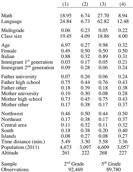
Table 1 shows summary statistics for our samples. For second graders, the average score on the mathematics standardized test is around 19 points (out of 32, or about 59 percent of correct answers), and it reaches 25 points (out of 39, or about 64 percent of correct answers) for the language test. Six percent of students attend a multigrade class, and class size is around 19 pupils per class. For fifth graders, the average performance on the mathematics standardized test is around 28 points (out of 47, or about 59 percent of correct answers), and it reaches 63
points (out of 82, or about 77 percent of correct answers) for the language test. Around 5 percent of students attend a multigrade class, and class size is around 19 pupils per class.
Besides age, children’s characteristics are similar across the two samples of second and fifth graders. Samples are balanced in terms of gender and around 11–12 percent of the children have an immigrant background. In terms of socioeconomic background, we consider three different levels of parental education: completed university, completed high school, and less than a secondary education diploma. Similar patterns emerge when we compare fathers and mothers. More than 70 percent of children in our samples come from families in which parents have at most an upper-secondary education. The percentage of university graduates is always lower than 10 percent, and 17–18 percent of parents have less than a high school education.
The bottom panel of Table 1 provides useful information about the geographical characteristics of the schools. The sample covers the entire Italian territory and all five macro-regions (Nomenclature of Territorial Units for Statistics, NUTS 1) are represented. The Northwestern area is the most represented (44–46 percent), followed by the South (18–20 percent), the Northeast (17 percent), the Central area (11 percent), and the Islands (8 percent). Unsurprisingly, municipalities where the schools are located are relatively small, with fewer than 5,000 inhabitants on average.
IV. The Identification Strategy
The IV identification strategy builds on the research design in Angrist and Lavy (1999), which is often referred to as the Maimonides’ Rule.viii In this work, the authors exploit class
size cutoffs imposed by a rule in Israel to estimate the impact of class size on scholastic achievement.
We take advantage of DPR 81/2009, a law that defines a set of exogenous cutoffs in terms of students of the same grade in a school to establish whether a new single or multigrade class should be created. Specifically, we use predicted-by-the-law grade composition of classes as well as predicted-by-the-law class sizes to instrument the actual grade composition of classes and class sizes, respectively.
In our estimates we carefully focus on class size, as estimating the multigrade effect is complicated by the possible impact of class size on student achievement. Class size is potentially correlated with the probability of attending multigrade classes and, at the same time, it can independently affect a child’s learning process. To account for possible class size effects, we implement a triple approach. First, we consider a model that excludes class size from the explanatory variables of student achievement. Second, we include class size as a control variable in our baseline specification. Third, as class size might suffer from the same sources of endogeneity as multigrading, we replicate our approach and treat it as an extra endogenous variable in the model.
DPR 81/2009 allows us to create four different instruments, defined as indicators for intervals in the number of students of the same grade enrolled in a specific school. The first indicator (I[CohortSize<10]) pertains to schools with fewer than 10 students in one grade. In this case, no single-grade class should be created, and all students in that grade should be assigned to a multigrade class.ix The second indicator (I[10≤CohortSize<15]) covers schools
with 10–14 students in one grade. In this interval both a single or a multigrade class could be created. The third indicator (I[15≤CohortSize<27]) covers schools with 15–26 students. In this case, the probability of assignment to a multigrade class should be close to zero. The same applies for the last indicator (I[CohortSize≥27]), which contains schools with more than 26 students in one grade. The number of students is too high to create a multigrade class; therefore,
according to the law, more than one single-grade class should be created for students in that grade.
The validity of our instrumental approach relies on a set of assumptions. To avoid violating the exclusion restriction, we need our instruments to only affect students’ test scores via grade composition (single versus multigrade class) and class size. Due to the characteristics of the enrollment process in primary school, the exact number of students enrolled in a specific grade is unpredictable as in Italy each family is free to enroll children in every school nationwide, although students living in schools’ catchment area have priority. Moreover, the enrollment procedure and its timing make it particularly difficult, if not impossible, for parents to form reliable expectations about the probability of their child’s ending up in a class with specific characteristics in terms of size and grade composition. A second important assumption underlying the literature based on Maimonides-style IV approaches is the absence of ad hoc manipulation around cutoffs. As shown in Section V.A, we do not find evidence of such manipulation.
Under these assumptions we define the following reference model: (1) TestScoreisj = β1Multigradeisj + β2ClassSizeisj +𝐗𝐢𝐬𝐣′ 𝛃𝟑 + αj + uisj ,
where i, s, and j stand for student, school, and geographical macro-area, respectively. TestScore is the student’s performance on the standardized national INVALSI test. We will focus on test scores at the end of the second and fifth grades of primary school. Specifically, the outcome variable is the combination of math and language INVALSI standardized test scores. After normalizing both test scores with a mean of zero and a standard deviation of one, we create a combined score in math and reading, taking the average of the normalized reading and math scores. We then normalize the combined score.x Multigrade is a dummy variable that takes the
value of one if the student attends a multigrade class, and ClassSize represents the student’s class size.
The vector X contains observable factors likely to affect test scores. Specifically, we control for child characteristics such as age, gender, and nationality by distinguishing native Italians, first-generation immigrants, and second-generation immigrants. We proxy parental background by including in the model both the father’s and mother’s education (university graduate versus high school graduate versus other) and profession.xi
The vector X also includes information about the population and the altitude of the municipality hosting the school, and the minimum car travel time needed to reach the closest alternative primary school from the school each student actually attends. Travel time to the closest school indicates the presence of alternative school options. If alternative primary schools are available, parents who dislike multigrade classes and who expect their child to end up in such a class might decide to enroll their child in the closest school offering single-grade classes. For this reason, we include this measure of travel distance in all our models.xii Finally, to
consider geographical differences across the country, we include in our model a set of macro-region fixed effects (αj) that capture the average effect on test score for regions in the Northwest,
the Northeast, the Central area, the South, and the Islands.
We estimate two different IV specifications defining two different sets of first stages. In one specification, we only instrument Multigrade and we either exclude ClassSize to estimate the raw effect of attendance in a multigrade class or use it as a standard control variable. The first stage for the case with class size as a control variable is defined as:xiii
(3) Multigradeisj = γ1I[CohortSize<10]s + γ2I[10≤CohortSize<15]s +
In the model including ClassSize as an additional endogenous variable, we replicate the same first stage as in Equation 2 and then add a first stage of the following form:
(4) ClassSizeisj = δ1I[CohortSize<10]s + δ2I[10≤CohortSize<15]s +
δ3I[15≤CohortSize<27]s + δ4I[CohortSize≥27]s + 𝐗𝐢𝐬𝐣′ 𝛅𝟓 + αj + µisj .
Because of possible serial correlation of the error term at the school level, all the models are estimated with standard errors clustered at the school level.
V. The Effect of Multigrading on Child Achievement
In this section we present first-stage estimates, the main results concerning the effect of multigrading on students’ achievements, and finally, we analyze possible heterogeneous effects of attendance in a multigrade class.
A. First-Stage Estimates
A typical concern related to the adoption of Maimonides-style rules is possible ad hoc manipulation around the cutoff to prevent the enforcement of specific class or grade composition. We deal with this concern by comparing observable individual characteristics around the three relevant cutoffs (10, 15, and 27 students). Tables 2 and 3 report the analysis of a relevant set of children’s individual characteristics (age, gender, nationality) and family characteristics (parental education) for second and fifth graders, respectively. We impose a two-student-interval around each cutoff, comparing, for instance, schools with 8 or 9 students with schools with 10 or 11 students. All the average values are remarkably similar around the cutoffs. The p-values for the differences in means in column (4) of both tables suggest the lack of manipulation by school principals.xiv
Having addressed the manipulation concern, we rationalize our instrumental variable approach in Figure 1. For each grade of interest, we provide a graphical representation of the
relation between the instruments and the two endogenous variables of the model, namely grade composition and class size. The figure in each panel contains bins representing the average y-value for each ventile of the distribution of the number of enrolled students in the school. Vertical lines display the cutoffs in terms of enrolled students that define the intervals used as instruments, and the solid horizontal lines represent the average y-value for each interval.
We start with the relation between the predicted probability of attending a multigrade class computed as in Equation 3 and the number of students enrolled in a certain grade in the school. Figures 1a and 1c for second and fifth graders, respectively, highlight that students in schools with fewer than 10 second or fifth graders have a high predicted probability (around 80 percent) of attending a multigrade class. The probability is lower (15–19 percent) for the interval of 10– 14 students. The probability drops to zero for the last two intervals, 15–26 students and more than 26 students, identified by the law.
Figures 1b and 1d depict the relation between class size and the number of enrolled students in a specific grade. Figure 1b refers to second graders, and Figure 1d illustrates the case of fifth graders. The 10-student cutoff imposed by the law does not affect class size. Indeed, class size remains similar around the cutoff. On the contrary, average class size increases for schools with more than 14 students and remains similar around the 27-student cutoff.
The graphical analysis in Figure 1 shows that our four instruments allow us to separately deal with the endogeneity of both multigrading and class size as they identify different margins along the cohort size distribution. A first margin identified by the 10-student cutoff mainly affects the individual probability of attendance in a multigrade class, and a second margin corresponding to schools with more than 14 students largely affects class size but has limited or no effect on multigrading.
Tables 4 and 5 show the first-stage estimates for second- and fifth-grade students, respectively. In the two tables, columns (1) and (2) report estimates for multigrading as the only endogenous variable excluding or including class size as a standard control, and columns (3) and (4) report results for the model considering class size as a further endogenous variable. In the latter case, column (3) reports first-stage estimates for multigrading, and column (4) shows first-stage results for class size. All the tests for under- and weak identification suggest that the first stage is very precise and the instruments are relevant.
For second graders, enrollment in a school with a number of enrolled students falling in the first two intervals (fewer than 10 second graders, 10–14 second graders) highly predicts the probability of attending a multigrade class. With respect to schools with more than 26 second graders (omitted category), students in schools with fewer than 10 second graders increase their probability of assignment to a multigrade class by more than 85 percentage points. This result is hardly surprising as the law forces the adoption of multigrade classes for these specific cases. The coefficient remains significant, but with a lower magnitude (0.15–0.19), for schools with 10–14 second graders. On the contrary, schools with 15–26 second graders display zero effect on the probability of assignment to a multigrade class.xv For fifth graders, the effect of the four instruments on the probability of attending a multigrade class is remarkably similar.
First-stage estimates for class size in column (4) of Tables 4 and 5 show that the first two intervals for enrolled (second- or fifth-grade) students report similar coefficients with respect to schools with more than 26 students: on average, class size decreases by around five students for schools with fewer than 10 students or 10–14 students. Schools with 15–26 students have, on average, an extra student per class compared to schools with more than 26 students.
The analysis of the first stage is important for unveiling the role of parental education in shaping the individual probability of attending a multigrade class. Students of parents reporting
a university degree display a zero and (in most cases) statistically insignificant increase in the likelihood of attendance in a multigrade class as opposed to students of parents with at most a high school diploma. This finding confirms that parents are unlikely to understand the individual probability of their children’s assignment to a multigrade class or, alternatively, that their background does not systematically shape their preferences on this matter.
B. Second-Stage Estimates
We start with the graphical representation of reduced-form effects of our instruments on the measure for child cognitive achievement, namely, the combined math-language test score.xvi In Figure 2, we visually represent the relation between test scores and the number of enrolled second (Figure 2a) and fifth graders (Figure 2b) in each school. Each figure contains bins representing the average test score for each ventile of the distribution of the number of students enrolled. Vertical lines display the cutoffs defining intervals used as instruments, and the solid horizontal lines represent the average test score for each interval.
As previously discussed, the first two intervals around the 10-student cutoff suggest a reduced-form effect on test score induced by attendance in a multigrade class. The evidence for second graders suggests a sizable positive impact of multigrading. The average value of the cognitive score for students below the 10-student cutoff (those students who are highly likely to attend a multigrade class), is almost double the score for students in the following interval (10–14 students). The second two intervals for schools with more than 14 second graders depict the reduced-form effects of class size on performance. Class size negatively affects a student’s performance: the average test score for students from schools with more than 14 second graders is lower than the one for students from smaller schools.
For fifth graders, the effect of multigrading on scholastic performance seems close to zero. Some evidence of the negative class size effect arises, although it is less evident than for second graders.
Table 6 shows second-stage estimates of the model in Equation 1 for the samples of second graders (columns 1–4) and fifth graders (columns 5–8). For each sample, we estimate the reference OLS model (columns 1 and 5), the IV model providing the raw effect of multigrading without controlling for class size (columns 2 and 6), the IV model with class size as a control variable (columns 3 and 7), and the IV model with class size as an endogenous variable (columns 4 and 8).
Multigrading displays a positive effect on the performance of second-grade students. According to OLS estimates, attendance in a multigrade class increases the combined math-language test score by as much as 9 percent of a standard deviation. The IV analysis suggests a 24 percent of a standard deviation increase in the specification without the control for class size. This coefficient is the combination of the multigrade effect and the class size effect; therefore it is important to consider that multigrade classes have, on average, five to six fewer students than single-grade classes. The effect of multigrading on test scores reaches the value of 16–19 percent of a standard deviation when we include class size as a standard control variable or as an additional endogenous variable in the model.xvii
We do not find significant effects of multigrading for fifth graders. All specifications provide coefficients remarkably close to zero, either positive or negative, and never statistically significant at the usual confidence levels. The zero effect for fifth graders may be the result of: (i) students who were assigned to a multigrade class only in the fifth year of primary school; or (ii) students who attended more than one year in a multigrade class, so that their performance in the fifth (and last) year of primary school would represent the cumulative effect of attending
a multigrade class for multiple years. In the second case, the multigrade effect would sum up different important dimensions such as classroom grade compositions of multigrade classes and age of peers. We will discuss the interpretation of results for fifth graders in Section VI.B.
The class size effect is similar when we consider different specifications and samples. For both second and fifth graders, class size plays a significant role in affecting achievement: a one-student-per-class increase explains an average decrease in individual performance of around 1 percent of a standard deviation. It is important to note that point estimates for the effect of multigrading are almost unaffected by the inclusion of class size as a pure control or as an endogenous variable.
Our results are robust to a complete set of sensitivity tests performed in Section III.B of the Online Appendix.
C. Heterogeneous Effects of Multigrading
Is the effect of multigrading the same for all children? We propose here a heterogeneity analysis based on two important dimensions: gender and family background. Undeniably, the analysis of heterogeneous effects is always complicated in an IV setting. Instruments usually locally affect a fraction of the population, making it very difficult to compare different subpopulations. In our setting, the use of a law based on simple numerical rules to assign students to a single or multigrade class makes the analysis easier. Indeed, the instruments are also extremely powerful and relevant when using subsamples.
Table 7 shows the IV analysis by gender (columns 1–2) and by parental education (columns 3–4). The upper panel focuses on second-grade students, and the bottom panel reports results for fifth graders. Results by gender suggest that, although differences across genders are not striking, second-grade females seem to benefit from multigrading more than second-grade males. The coefficient for multigrading increases by almost 30 percent, from 17 to 22 percent
of a standard deviation, when comparing females to males. Results by gender for fifth graders confirm the statistically insignificant impact of multigrading.
In terms of parental background, we divide children in two groups according to their parents’ education. The low-parental education group (No one with university) includes children whose parents do not hold a university degree. The high-parental education group (One with university) includes children with at least one parent holding a university degree. For second graders, multigrading positively shapes children’s cognitive achievement for those with both types of parental backgrounds. However, the effect seems to be driven mainly by children from the low-parental education group. The coefficient for the low-parental education group is twice as large as the one for the high-parental education group (20 versus 9 percent of a standard deviation). Moreover, the coefficient for children with at least one parent with a university degree is statistically insignificant.xviii As for fifth graders, the analysis according to parents’ education confirms the zero effect stemming from multigrading.
The analysis of parental background highlights that very young children from less stimulating parental environments obtain the highest benefit from attendance in a multigrade class. This result identifies grade composition as a potential tool to mitigate the long-term effects of pupils’ lower socioeconomic backgrounds. A class environment consisting of older peers might partially compensate for the negative impact of low socioeconomic conditions for very young children.
VI. Investigating the Multigrade Effect
In this section we shed light on the potential mechanisms underlying the results of the baseline analysis. To this end, we focus on classroom grade composition, namely the age of peers sharing the class with students in a multigrade class. We start by focusing on
second-grade students. We then move to fifth second-graders and to the possible interpretations for the zero effect of multigrading on children’s cognitive achievement at this specific stage of primary school.
A. The Case of Second Graders: Younger is Better?
We replicate the baseline analysis by splitting the sample of second-grade students who attended a multigrade class into two different groups: students with only younger peers in the class and students with only older peers in the class.xix DPR 81/2009 does not provide specific rules guiding students’ assignments to multigrade classes with younger or older peers; the decision rests solely with the school principal and it is based on the cohort size for each grade in each year. Therefore, the number of students in adjacent grades usually drives this decision. This provides us with a source of variation to construct a new set of instruments for attendance in specific (in terms of grade composition) multigrade classes. As an example, the probability of a second-grade student attending a multigrade class with younger peers depends on her cohort size (second grade) and the size of the younger adjacent cohort (first grade). We use this combined information to construct instruments.
In detail, consider a case in which a second-grade student is enrolled in a school with fewer than 10 second graders. Now suppose that in the same school, the cohort size of first graders enrolled in the same SY is smaller than 15 students. In this specific case, the probability of the second graders ending up in a multigrade class with younger peers is considerably larger than in a case in which first graders are at least 15. With the same logic, we construct nine possible combinations suggested by the rules defined in DPR 81/2009, and we use indicators for these combinations as instruments for actual multigrading (and class size). For students in a multigrade class with younger peers, we consider first grade as the adjacent grade; for students sharing their class with older peers, we consider third grade as the adjacent grade.
Table 8 illustrates estimates for second graders by classroom grade composition. Columns (1–3) show the analysis for multigrade classes in which the students share the classroom with younger peers. Columns (4–6) show the analysis for those students with older peers in their classroom. Columns (1) and (4) report OLS estimates; columns (2–3) and (5–6) report the IV analysis.xx
The OLS estimates pinpoint a statistically insignificant 4 percent of a standard deviation effect of multigrading with younger peers on child achievement. The effect is considerably larger, 16 percent of standard deviation, for students sharing their class with older peers.
The IV estimates confirm a negligible effect of sharing classes with less-mature students. On the contrary, the presence of older peers in the class exerts a large and strongly significant positive effect on achievement that amounts to 32–33 percent of a standard deviation. Sharing the class with older peers might inspire and foster a child’s interactions with, and imitation of, her more-mature peers.
B. Interpretation of the Multigrade Effect for Fifth Graders
Students attending a multigrade class in their fifth (and last) year of primary school necessarily belong to the oldest cohort of the class. They may be having their first experience with multigrading; alternatively, they may have been in a multigrade class for several years during primary school. These two possible scenarios would affect the interpretation of multigrading’s zero impact. In the first scenario, the effect depends on attendance in a multigrade class during the last year of primary school, and consequently with younger peers in the class. In the second case, the multigrade effect would convey the cumulative effect of several years spent in a multigrade class. This interpretation would pinpoint the net effect of multigrading for primary school students who first experience multigrading as the youngest cohort and then as the oldest cohort in the class.
The analysis of these possible channels is particularly challenging as many different student career paths are possible. Hence, the definition of the proper counterfactual for fifth graders is far from univocal. Indeed, it is possible that the control group, namely the group of students attending a single-grade class during their fifth year of primary school, also includes some students who attended multigrade classes during their school career.
To deal with these potential concerns, we track back the grade composition of the primary school classes attended by fifth graders in our sample.xxi Figure 3 shows the number of years in a multigrade class for students attending a multigrade class in their fifth year of primary school in the 2012/2013 SY. The figure suggests the persistence of multigrading: fifth graders in a multigrade class are highly likely to have spent a considerable fraction of their primary school career in a multigrade class. About half of students experienced multigrading in all five years of their primary school career. Three-fourth of them ended up in a multigrade in at least four out of the five years. This evidence supports the idea that the zero effect of multigrading for fifth graders is likely to convey the cumulative impact of multigrading along the entire primary school cycle.
To gain further confidence about this interpretation, we exploit the fact that tracking the entire primary school career path of fifth graders allows us to define alternative and more precise versions of the control and treatment groups. All the analyses performed consider the test score at the end of primary school (fifth grade) as the outcome of interest. We start with the analysis of the effect of having attended at least one year of multigrading during primary school. The control group consists of those students who never attended a multigrade class; the treatment group consists of those students who experienced at least one year of multigrading.xxii In this case, we obtain IV estimates with instruments based on the average of each student’s
cohort size over the five years of primary school. We then apply the standard rules defined by DPR 81/2009 to the average cohort size.
Estimates in Table 9 display a zero effect of attendance in at least one year of multigrading during primary school on student achievement at the end of primary school. This result reinforces the interpretation that multigrading is a practice that is (at least) nondetrimental for the cognitive achievement of children who experienced several years of multigrading.
We extend the analysis in Table 10 by considering three different treatment groups: (i) students who attended a multigrade class exclusively in the last year of primary school (column 1), (ii) students who attended a multigrade class exclusively in the fourth or fifth year (or both) of primary school (column 2), and (iii) students who attended a multigrade class exclusively in the first or second year (or both) of primary school (column 3). We compare each of these groups with a control group consisting of those students who never attended a multigrade class during primary school. Unfortunately, persistence in multigrading limits the sample sizes for these groups and this limitation largely affects the precision of IV estimates. For this reason, we only propose a suggestive correlation analysis based on OLS estimates.
Table 10 shows that the correlation between assignment to a multigrade class exclusively in the last years of primary school and students’ achievement, although never statistically significant, is negative. These are the years in which the child is very likely to be part of the oldest cohort in the class. The multigrade coefficient turns to a positive value of 11 percent of a standard deviation for those students who experienced multigrading only at the very beginning of their career in primary school.
The analysis of fifth graders shown in Tables 9 and 10 is consistent with the view that given the persistence of multigrading for most students, the zero effect on fifth graders is likely to result from the combination of a possible positive effect when the child belongs to the youngest
cohort versus a possible negative effect when the child becomes part of the oldest cohort in the class.
The results for students who were in multigrade classes exclusively in the first years of primary school also allow us to infer some insights about the possible medium-run effects of multigrading. In this framework, we consider attendance in multigrade classes when the child is enrolled in her first or second grade, but test scores are measured when the child has reached the fifth grade. The 11 percent of a standard deviation effect of multigrading, although statistically insignificant, is remarkably similar to the OLS estimates of the effect of multigrading for second-grade students in Table 6. This similarity suggests some persistence of the positive effect of multigrading for those students attending multigrade classes only as younger peers in the classroom. However, this result only represents preliminary suggestive evidence; further and more precise analysis on the possible medium- and long-run effects of attendance in multigrading classes is needed.
VII. Conclusion
Multigrading, the practice of placing children of different ages in the same classroom, is a common educational practice in both developing and developed countries. Although in developing countries multigrading is widespread, in developed countries, multigrading is generally confined to rural areas with a declining population and where few children actually live. Nonetheless, over the last few years, several developed countries have adopted multigrading for educational and pedagogical reasons.
In this paper, we show that multigrading positively affects cognitive achievement of second graders in Italian primary schools. The effect for fifth graders is close to zero. We rationalize these findings by showing that the effect of multigrading is likely positive for
younger students sharing their class with older peers. On the other hand, the multigrade effect seems negative when the student belongs to the oldest cohort in the class. These opposite-in-sign effects explain the net-zero multigrade effect for fifth graders who, in the Italian primary school, usually experience multigrading as both the youngest cohort (the first grades) and the oldest cohort (the last grades) in the class.
Our results also highlight that the positive multigrade effect for second graders is stronger for children from low socioeconomic backgrounds. These children, who are exposed to peers of different ages through multigrading, receive important additional inputs that partially compensate for less stimulating home environments.
This work suggests at least two relevant policy implications. First, when considering cognitive development, multigrading implies potential beneficial effects when less-mature peers share their classroom with more-mature peers. Additionally, we do not find evidence of detrimental effects for those children who experienced several years of multigrading.
Second, multigrading is typical in schools in rural and remote areas still common in many countries. These areas often face low population density, deprivation, and abandonment by younger generations, which leads to poor economic conditions. Multigrading may be the only way to keep schools open in these areas, and schools are likely to be the only institution that can potentially revitalize them.
References
Agostinelli, Francesco, and Giuseppe Sorrenti. 2018. “Money vs. Time: Family Income, Maternal Labor Supply, and Child Development.” HCEO Working Paper 2018-017. Angrist, Joshua D., and Victor Lavy. 1999. “Using Maimonides’ Rule to Estimate the Effect
of Class Size on Scholastic Achievement.” The Quarterly Journal of Economics 114(2):533–75.
Angrist, Joshua D., Victor Lavy, Jetson Leder-Luis, and Adi Shany. 2019. “Maimonides Rule Redux.” American Economic Review: Insights (forthcoming).
Bonesrønning, Hans. 2003. “Class Size Effects on Student Achievement in Norway: Patterns and Explanations.” Southern Economic Journal 69(4):952–65.
Checchi, Daniele, and Maria De Paola. 2018. “The Effect of Multigrade Classes on Cognitive and Non-Cognitive Skills. Causal Evidence Exploiting Minimum Class Size Rules in Italy.” Economics of Education Review 67:235–53.
Cunha, Flavio, and James J. Heckman. 2008. “Formulating, Identifying and Estimating the Technology of Cognitive and Noncognitive Skill Formation.” Journal of Human
Resources 43(4):738–82.
Cunha, Flavio, James J. Heckman, and Susanne M. Schennach. 2010. “Estimating the Technology of Cognitive and Noncognitive Skill Formation.” Econometrica 78(3):883– 931.
Dahl, Gordon B., and Lance Lochner. 2012. “The Impact of Family Income on Child
Achievement: Evidence from the Earned Income Tax Credit.” American Economic Review 102(5):1927– 56.
Dobbelsteen, Simone, Jesse Levin, and Hessel Oosterbeek. 2002. “The Causal Effect of Class Size on Scholastic Achievement: Distinguishing the Pure Class Size Effect from the Effect
of Changes in Class Composition.” Oxford Bulletin of Economics and Statistics 64(1):17– 38.
Gary-Bobo, Robert J., and Mohamed B. Mahjoub. 2013. “Estimation of Class-Size Effects, Using ‘Maimonides’ Rule’ and Other Instruments: The Case of French Junior High Schools.” Annals of Economics and Statistics (111/112):193–225.
Hargreaves, Eleonore, Juan C. Montero, Huy N. Chau, M. Sibli, and Nguyen T. Thanh. 2001. “Multigrade Teaching in Peru, Sri Lanka and Vietnam: An Overview.” International
Journal of Educational Development 21(6):499–520.
Hoxby, Caroline M. 2000. “The Effects of Class Size on Student Achievement: New
Evidence from Population Variation.” The Quarterly Journal of Economics 115(4):1239– 85.
Leuven, Edwin, Hessel Oosterbeek, and Marte Rønning. 2008. “Quasi-Experimental
Estimates of the Effect of Class Size on Achievement in Norway.” Scandinavian Journal
of Economics 110(4):663–93.
Leuven, Edwin, and Marte Rønning. 2016. “Classroom Grade Composition and Pupil Achievement.” The Economic Journal 126(593):1164–92.
Little, Angela W. 2001. “Multigrade Teaching: Towards an International Research and Policy Agenda.” International Journal of Educational Development 21(6):481–97.
Materiali Uval. 2014. “A Strategy for Inner Areas in Italy: Definition, Objectives, Tools and Governance.” In Analisi e studi, Documenti, Metodi, eds. Fabrizio Barca, Paola Casavola, and Sabrina Lucatelli, Materiali Uval.
Mulkeen, Aidan G., and Cathal Higgins. 2009. “Multigrade Teaching in Sub-Saharan Africa: Lessons from Uganda, Senegal, and the Gambia.” World Bank Working Paper 173. UNESCO (2004). “Educating Rural People: a Low Priority.” Education Today, 9.
Table 1 Summary Statistics Mean (1) St.Dev. (2) Mean (3) St.Dev. (4) Math 18.95 6.74 27.70 8.94 Language 24.84 6.73 62.82 12.48 Multigrade 0.06 0.23 0.05 0.22 Class size 19.45 4.09 18.86 4.00 Age 6.97 0.27 9.98 0.32 Female 0.49 0.50 0.50 0.50 Italian 0.88 0.32 0.89 0.31 Immigrant 1st generation 0.03 0.17 0.05 0.21 Immigrant 2nd generation 0.09 0.28 0.06 0.24 Father university 0.07 0.26 0.06 0.24 Father high school 0.75 0.44 0.76 0.43
Father other 0.18 0.39 0.18 0.38
Mother university 0.10 0.30 0.08 0.28 Mother high school 0.73 0.45 0.75 0.43
Mother other 0.17 0.38 0.17 0.37 Northwest 0.46 0.50 0.44 0.50 Northeast 0.17 0.38 0.17 0.37 Central area 0.11 0.32 0.11 0.32 South 0.18 0.38 0.20 0.40 Islands 0.08 0.27 0.08 0.27
Time distance (min.) 5.49 3.30 5.58 3.36 Population (2011) 4,673 3,097 4,609 3,057
Altitude 261 222 268 227
Sample 2nd Grade 5th Grade
Observations 92,469 89,780
Notes: Summary statistics for the samples analyzed in this work. Columns (1) and (2) refer to the sample of second-grade students; columns (3) and (4) refer to the sample of fifth-grade students.
Table 2
Balancing Test for Second-Grade Students
Below Cutoff (BC) (1) Above Cutoff (AC) (2) BC-AC (3) p-value (BC-AC) (4) First cutoff: 10 students
Age 6.96 6.95 0.01 0.58 (0.01) (0.01) (0.01) Female 0.48 0.49 -0.01 0.53 (0.01) (0.01) (0.02) Italian 0.90 0.90 0.00 0.66 (0.01) (0.01) (0.01) Father university 0.05 0.06 -0.01 0.82 (0.01) (0.01) (0.01) Mother university 0.08 0.09 -0.01 0.36 (0.01) (0.01) (0.01) Number of students [8,9] [10,11]
Second cutoff: 15 students
Age 6.96 6.96 0.00 0.57 (0.01) (0.01) (0.01) Female 0.47 0.49 -0.02 0.18 (0.01) (0.01) (0.01) Italian 0.90 0.90 0.00 0.75 (0.01) (0.01) (0.01) Father university 0.06 0.05 0.01 0.10 (0.00) (0.00) (0.01) Mother university 0.10 0.10 0.00 0.98 (0.01) (0.01) (0.01) Number of students [13,14] [15,16]
Third cutoff: 27 students
Age 6.97 6.95 0.02 0.06 (0.01) (0.01) (0.01) Female 0.49 0.48 0.01 0.46 (0.01) (0.01) (0.01) Italian 0.90 0.88 0.02 0.06 (0.01) (0.01) (0.01) Father university 0.06 0.07 -0.01 0.01 (0.00) (0.01) (0.01) Mother university 0.09 0.10 -0.01 0.15 (0.01) (0.01) (0.01) Number of students [25,26] [27,28]
Notes: Comparison of students’ characteristics just below (column 1) and just above (column 2) the three critical cutoffs of second-grade (enrolled) students identified by DPR 81/2009. The critical cutoffs are 10, 15, and 27 students. Interval widths around the cutoffs are defined by two students above/below, that is, 8–9 students versus 10–11 students. The difference in means and the p-value for difference in means are reported in columns (3) and (4),
Table 3
Balancing Test for Fifth-Grade Students
Below Cutoff (BC) (1) Above Cutoff (AC) (2) BC-AC (3) p-value (BC-AC) (4) First cutoff: 10 students
Age 9.94 9.95 -0.01 0.20 (0.01) (0.01) (0.01) Female 0.51 0.49 0.02 0.19 (0.01) (0.01) (0.02) Italian 0.92 0.90 0.02 0.01 (0.01) (0.01) (0.01) Father university 0.05 0.05 0.00 0.98 (0.00) (0.00) (0.01) Mother university 0.07 0.08 -0.01 0.39 (0.01) (0.01) (0.01) Number of students [8,9] [10,11]
Second cutoff: 15 students
Age 9.97 9.96 0.01 0.30 (0.01) (0.01) (0.01) Female 0.50 0.50 0.00 0.94 (0.01) (0.01) (0.01) Italian 0.91 0.91 0.00 0.77 (0.00) (0.00) (0.01) Father university 0.05 0.06 -0.01 0.23 (0.00) (0.00) (0.01) Mother university 0.07 0.08 -0.01 0.31 (0.00) (0.00) (0.01) Number of students [13,14] [15,16]
Third cutoff: 27 students
Age 9.96 9.97 -0.01 0.52 (0.01) (0.01) (0.01) Female 0.49 0.51 -0.02 0.16 (0.01) (0.01) (0.01) Italian 0.90 0.89 0.01 0.55 (0.01) (0.01) (0.01) Father university 0.06 0.05 0.01 0.59 (0.00) (0.00) (0.01) Mother university 0.08 0.08 0.00 0.39 (0.01) (0.01) (0.01) Number of students [25,26] [27,28]
Notes: Comparison of students’ characteristics just below (column 1) and just above (column 2) the three critical cutoffs of fifth-grade (enrolled) students identified by DPR 81/2009. The critical cutoffs are 10, 15, and 27 students. Interval widths around the cutoffs are defined by two students above/below, that is, 8–9 students versus 10–11 students. The difference in means and the p-value for difference in means are reported in columns (3) and (4), respectively.
Table 4
First-Stage Estimates for Second-Grade Students
Model (1) Model (2) Model (3)
Multigrade OLS (1) Multigrade OLS (2) Multigrade OLS (3) Class size OLS (4) I [2ndGraders < 10] 0.86*** 0.90*** 0.86*** -5.19*** (0.01) (0.01) (0.01) (0.20) I [10 ≤ 2ndGraders < 15] 0.15*** 0.19*** 0.15*** -5.44*** (0.01) (0.02) (0.01) (0.18) I [15 ≤ 2ndGraders < 27] -0.00 -0.01*** -0.00 0.97*** (0.00) (0.00) (0.00) (0.17) Class size 0.01*** (0.00) Father university -0.00 -0.00 -0.00 -0.03 (0.00) (0.00) (0.00) (0.05) Mother university -0.00 -0.00 -0.00 -0.01 (0.00) (0.00) (0.00) (0.04) SW Chi-sq. (UId) > 100 > 100 > 100 > 100 p-value 0.00 0.00 0.00 0.00 SW F (WId) > 100 > 100 > 100 > 100 p-value 0.00 0.00 0.00 0.00 KP (WId) > 100 > 100 > 100 > 100 F-stat (I [2ndGr. < 10]) > 100 > 100 > 100 > 100 F-stat (I [10 ≤ 2ndGr. < 15]) > 100 > 100 > 100 > 100 F-stat (I [15 ≤ 2ndGr. < 27]) 0.14 10.23 0.14 31.28
Instrumented variable(s) Multigrade Multigrade Multigrade,
Class size
Sample 2nd Grade 2nd Grade 2nd Grade 2nd Grade
Observations 92,469 92,469 92,469 92,469
Notes: First-stage estimates for second-grade students. Dependent variable: Attendance in a multigrade class (columns 1, 2, and 3), class size (column 4). Model (1) does not include class size as a control variable. Model (2) includes class size as a control variable. Model (3) treats both multigrade and class size as endogenous variables. The reference category for the number of second-grade students is I[2ndGraders ≥ 27]. The reference category for
father’s and mother’s education is completed high school. All models include controls for child’s gender, age, nationality, and father’s and mother’s profession. All models also include variables for altitude and population of the municipality, geographical macro-area, and road distance in time to the closest alternative school. Standard errors are clustered at the school level and reported in brackets.
Table 5
First-Stage Estimates for Fifth-Grade Students
Model (1) Model (2) Model (3)
Multigrade OLS (1) Multigrade OLS (2) Multigrade OLS (3) Class size OLS (4) I [5thGraders < 10] 0.79*** 0.83*** 0.79*** -5.06*** (0.02) (0.01) (0.02) (0.20) I [10 ≤ 5thGraders < 15] 0.10*** 0.15*** 0.10*** -4.97*** (0.01) (0.01) (0.01) (0.16) I [15 ≤ 5thGraders < 27] -0.00 -0.01*** -0.00 1.09*** (0.00) (0.00) (0.00) (0.18) Class size 0.01*** (0.00) Father university -0.00* -0.00* -0.00* -0.01 (0.00) (0.00) (0.00) (0.05) Mother university -0.00 -0.00 -0.00 -0.06 (0.00) (0.00) (0.00) (0.04) SW Chi-sq. (UId) > 100 > 100 > 100 > 100 p-value 0.00 0.00 0.00 0.00 SW F (WId) > 100 > 100 > 100 > 100 p-value 0.00 0.00 0.00 0.00 KP (WId) > 100 > 100 > 100 > 100 F-stat (I [5thGr. < 10]) > 100 > 100 > 100 > 100 F-stat (I [10 ≤ 5thGr. < 15]) 86.66 > 100 > 100 > 100 F-stat (I [15 ≤ 5thGr. < 27]) 2.58 23.06 2.58 38.64
Instrumented variable(s) Multigrade Multigrade Multigrade,
Class size
Sample 5th Grade 5th Grade 5th Grade 5th Grade
Observations 89,780 89,780 89,780 89,780
Notes: First-stage estimates for fifth-grade students. Dependent variable: Attendance in a multigrade class (columns 1, 2, and 3), class size (column 4). Model (1) does not include class size as a control variable. Model (2) includes class size as a control variable. Model (3) treats both multigrade and class size as endogenous variables. The reference category for the number of fifth-grade students is I[5thGraders ≥ 27]. The reference category for father’s and mother’s education is completed high school. All models include controls for child’s gender, age, nationality, and father’s and mother’s profession. All models also include variables for altitude and population of the municipality, geographical macro-area, and road distance in time to the closest alternative school. Standard errors are clustered at the school level and reported in brackets.
Table 6
Multigrading and Child Achievement
Combined Math-Language OLS (1) IV (2) IV (3) IV (4) OLS (5) IV (6) IV (7) IV (8) Multigrade (M) 0.09*** 0.24*** 0.16*** 0.19*** -0.02 0.05 0.01 -0.01 (0.03) (0.04) (0.04) (0.05) (0.03) (0.04) (0.04) (0.05) Class size (CS) -0.01*** -0.01*** -0.01 -0.01** -0.01** -0.01 (0.00) (0.00) (0.01) (0.00) (0.00) (0.00) E(C S|M = 0)− E(C S|M = 1) 5.94 5.94 5.94 5.94 5.30 5.30 5.30 5.30
Instrumented Multigrade Multigrade Multigrade, Multigrade Multigrade Multigrade,
variable(s) Class size Class size
Sample 2nd Grade 2nd Grade 2nd Grade 2nd Grade 5th Grade 5th Grade 5th Grade 5th Grade
Observations 92,469 92,469 92,469 92,469 89,780 89,780 89,780 89,780
Notes: Analysis of the effect of multigrading on a child’s test score. Dependent variable: Combined Math-Language test score. Columns (2) and (6) do not include class size as a control variable. Columns (3) and (7) include class size as a control variable. Columns (4) and (8) treat both multigrade and class size as endogenous variables. Columns (1) to (4) refer to second-grade students. Columns (5) to (8) refer to fifth-grade students. Columns (2) and (6) do not include class size as a control variable. Columns (3) and (7) include class size as a control variable. Columns (4) and (8) treat both multigrade and class size as endogenous variables. All models include controls for child’s gender, age, nationality, father’s and mother’s educational level, and father’s and mother’s profession. All models also include variables for altitude and population of the municipality, geographical macro-area, and road distance in time to the closest alternative school. E(CS|M = 0) − E(CS|M = 1) represents the difference in the average class size (number of students) between single-grade classes (M = 0) and multigrade classes (M = 1). Standard errors are clustered at the school level and reported in brackets.
Table 7
Heterogeneous Effects of Multigrading on Child Achievement
Combined Math-Language
Child’s gender Parental education
IV (1) IV (2) IV (3) IV (4)
Female Male No one with
university One with university Multigrade 0.22*** 0.17*** 0.20*** 0.09 (0.06) (0.06) (0.05) (0.07) Class size -0.01 -0.01 -0.01 -0.01 (0.01) (0.01) (0.01) (0.01) Instrumented variables Multigrade, Class size Multigrade, Class size Multigrade, Class size Multigrade, Class size
Sample 2nd Grade 2nd Grade 2nd Grade 2nd Grade
Observations 45,224 47,245 79,856 12,613
Female Male No one with
university One with university Multigrade 0.03 -0.05 -0.02 0.06 (0.05) (0.06) (0.05) (0.09) Class size -0.01 -0.01 -0.01* 0.00 (0.01) (0.01) (0.01) (0.01) Instrumented variables Multigrade, Class size Multigrade, Class size Multigrade, Class size Multigrade, Class size
Sample 5th Grade 5th Grade 5th Grade 5th Grade
Observations 44,875 44,905 79,262 10,518
Notes: Heterogeneous IV estimates by child’s gender (columns 1 and 2) and parental education (columns 3 and 4). Dependent variable: Combined Math-Language test score. The upper panel refers to second-grade students. The lower panel refers to fifth-grade students. All models include controls for child’s gender (except columns 1 and 2), age, nationality, father’s and mother’s educational level (except columns 3 and 4), and father’s and mother’s profession. All models also include variables for altitude and population of the municipality, geographical macro-area, and road distance in time to the closest alternative school. Standard errors are clustered at the school level and reported in brackets.
Table 8
Classroom Grade Composition and Child Achievement
Combined Math-Language OLS (1) IV (2) IV (3) OLS (4) IV (5) IV (6) Multigrade 0.04 0.11* 0.10 0.16*** 0.33*** 0.32*** (0.04) (0.06) (0.07) (0.05) (0.09) (0.10) Class size -0.01*** -0.01*** -0.01** -0.01*** -0.01*** -0.01** (0.00) (0.00) (0.00) (0.00) (0.00) (0.00) Instrumented variable(s) Multigrade Multigrade,
Class size Multigrade
Multigrade, Class size
In multigrade with Younger
peers Younger peers Younger peers Older peers Older peers Older peers
Sample 2nd Grade 2nd Grade 2nd Grade 2nd Grade 2nd Grade 2nd Grade
Observations 89,461 89,461 89,461 88,428 88,428 88,428
Notes: Analysis of the effect of multigrading for second-grade students by classroom grade composition. Dependent variable: Combined Math-Language test score. Younger peers (columns 1, 2, and 3) means that only first-grade students attend the same multigrade class of second-grade students. Older peers (columns 4, 5, and 6) means that students of higher grades (third, fourth, and fifth grades) attend the same multigrade class of second-grade students. Instruments used in columns (2) and (3) are indicators for different intervals in the joint distribution of first-grade and second-grade (enrolled) students. Instruments used in columns (5) and (6) are indicators for different intervals in the joint distribution of second-grade and third-grade (enrolled) students. Refer to the text for further details and to Online Appendix Section IV for first-stage estimates. All models include controls for child’s gender, age, nationality, father’s and mother’s educational level, and father’s and mother’s profession. All models also include variables for altitude and population of the municipality, geographical macro-area, and road distance in time to the closest alternative school. Standard errors are clustered at the school level and reported in brackets.
Table 9
The Effect of Spending at Least One Year in a Multigrade Class
Combined Math-Language OLS (1) IV (2) IV (3) At least one year in multigrade -0.01 0.01 -0.04
(0.03) (0.03) (0.05) Class size -0.01** -0.01** -0.01** (0.00) (0.00) (0.01) Instrumented variable(s) Multigrade Multigrade, Class size
Sample 5th Grade 5th Grade 5th Grade Observations 88,861 88,861 88,861
Notes: Analysis of the effect of spending at least one year in multigrading during primary school on a child’s test score in the fifth grade. Dependent variable: Combined Math-Language test score. The analysis is obtained by tracking back the entire primary school career of fifth-grade students. Instruments are obtained by averaging each student’s cohort size over the five years of primary school. The rules established by DPR 81/2009 are then applied to the average cohort size as in the rest of the paper to obtain the instruments. Refer to the text for further details on instruments construction. All models include controls for child’s gender, age, nationality, father’s and mother’s educational level, and father’s and mother’s
profession. All models also include variables for altitude and population of the municipality, and road distance in time to the closest alternative school. Standard errors are clustered at the school level and reported in brackets.