Volume 29, Issue 2
Comparing shapes of engel curves
Andreas Chai
Productivity Commission, Australian Government
Alessio Moneta
Max Planck Institute of Economics, Jena
Abstract
We measure how different the shapes of Engel curves are across 59 commodity groups. The same analysis is carried out for their derivatives and variances. While Engel curves possess a relatively homogeneous shape, significantly more heterogeneity is present in derivatives and when particular sub-classes of income are considered.
We thank Nancy Heckman, Nadine Chlaß, and the participants of the Evolutionary Economics group seminar at MPI for useful suggestions. We also thank Sebastian Müller and Michael Enukashvili for research assistance. We retain responsibility for any error.
Citation: Andreas Chai and Alessio Moneta, (2009) ''Comparing shapes of engel curves'', Economics Bulletin, Vol. 29 no.2 pp. 1156-1162. Submitted: Feb 09 2009. Published: May 28, 2009.
1
Introduction
Engel curves (ECs) capture a fundamental aspect of consumer behavior: the sensitivity of con-sumption to income. However, there is significant variation in how concon-sumption expenditures react to changes in income across different commodity groups (see among others Prais 1953, Aitchison and Brown 1954). Nonparametric methods have been used to tackle this hetero-geneity since they do not require researchers to impose any functional form in the estimation (see e.g. H¨ardle and Jerison 1991, Engel and Kneip 1996). In parallel, economic theory has developed new demand systems allowing for the observed diversity in expendituincome re-lationships (Banks et al. 1997, Blundell et al. 2007). Yet, no study so far has tried to measure the magnitude of this diversity across commodity expenditures. We assess to what extent ECs differ in shapes for a large variety of expenditure categories. To achieve this, we exploit the flexibility both in estimation and in curve comparison that nonparametric techniques provide. Our findings indicate that ECs do not differ much in shape. They do, however, substantially differ in terms of their derivative, which is the empirical analogue of the marginal propensity to consume one particular commodity. Intriguing differences are also found for sub-classes of income. We finally estimate the variance of expenditure at each point of income, shortly referred to as “ECs variance.” Each EC variance describes how the variability in consumption behavior depends on income for a given commodity group. Our findings reveal here noteworthy differences across commodity groups.
2
Data and Estimation Method
We use data from the U.K. Family Expenditure Survey 2001. The data set consists of family budgets related to 59 types of expenditures. These refer to housing costs (1 type of expendi-ture), fuel (2 types), food (14 types), alcohol (2 types), tobacco (2 types), clothing and footwear (5 types), household goods (7 types), domestic services (5 types), personal goods and services (6 types), motor expenditures (4 types), travel expenditures (3 types), TV, Books, Newspa-pers, etc. (4 types), entertainment and education (4 types). Expenditures are expressed in
British pounds.1
An EC is estimate for each type of expenditure g by regressing the level of expenditure Yi
for g on total expenditure Xi:
Yi = m(Xi) + ²i, (1)
for households i = 1, . . . , n.2 For this purpose we use the Gasser-M¨uller kernel type of
smooth-ing (Gasser and M¨uller 1984, Gasser et al. 1991). This choice has two reasons. First, this estimate has an asymptotic bias that is preferable to the Nadaraya-Watson method. Second, it is the most suited to estimating the derivatives of regression functions. We use a fourth-order kernel (necessary for derivative estimation) as weighting function. The bandwidth parameter is selected via the Herrmann’s (1997) plug-in approach, in order to deal with heteroscedastic-ity, which is a typical feature of expenditure data. The variance of Y at each point of X (EC variance) is estimated using the Engel and Kneip’s (1996: 204) binned convolution method.
1Sample sizes range from 173 (non-motor vehicles) to 6382 observations (cereals). The average sample size
is 3287.
2We normalize X to take values in [0, 1]. This is done dividing, for each category of commodity, both X i
3
Measure of Shape Similarity
To measure the similarity in shape between the estimated curves we use the rank correlation method proposed by Heckman and Zamar (2000). A comparative advantage of this method is the ability to capture qualitative features of the curves such as kinks and spikes. Methods
based on L2 distance do not perform well in this respect (Marron and Tsybakov 1995). The
rank correlation used here is a generalization of the rank correlation between two finite vectors of numbers (cf. Gibbons 1991). If two curves have the same shape our coefficient is equal to
one. Two curves y = m1(x) and y = m2(x) are said to have the same shape if there exists a
strictly increasing function g such that m1(x) = g{m2(x)}, that is the plot of y = m1(x) is the
same of y = m2(x) after a deformation of the y axis (Heckman and Zamar 2000: 136). The
Heckman-Zamar method presupposes the definition of a probability measure µ on the interval
in which m1(x) and m2(x) are defined (which is the unit interval after standardizing the data).
Our proposed measure is µ(A) = (#x ∈ A)/(#x ∈ [0, 1]) (i.e the proportion of x points that are in A), for any subinterval A of the unit interval. The rationale for using this measure is to give more weight to the portion of the curve for which there are more observations. The
rank correlation between m1(x) and m2(x) is defined as:
ρµ(m1, m2) = R {rm1(w) − Rm1}{rm2(w) − Rm2}dµ(w) qR {rm1(w) − Rm1}2dµ(w)R{rm2(w) − Rm2}2dµ(w) , (2) where rm1(x) = µ{t : m 1(t) < m1(x)} + 12µ{t : m1(t) = m1(x)} and Rm1 = R rm1(w)dµ(w).
rm2(x) and Rm2 are defined analogously. A consistent estimator of ρ
µ is given by Heckman
and Zamar (2000: 139).
4
Empirical Results
We measure to what extent ECs are similar in shape by calculating the distance d = (1 − ρµ)
for each pair of the 59 estimated ECs. Since −1 ≤ ρµ ≤ 1, 0 ≤ d ≤ 2. The same procedure
is applied to derivative and variance curves.3 The first important result is that there is more
variety in the shapes of derivatives than in the shapes of simple ECs and variances. This is evident when comparing the calculated distances between derivatives with both the calculated distances between ECs and those between variances. The second column of table 1 displays how the distances between ECs are distributed across different intervals. Specifically, 642 out of 1711 (= 59 · 58/2) pairs of ECs (37.5% of the total) consist of two curves distant 0 < d ≤ 0.01 from each other. In the same way, 519 (30.3%) pairs have a within distance 0.01 < d ≤ 0.1, 114 pairs have 0.1 < d ≤ 0.25, and so on. In contrast (see third column in table 1), the majority of pairs of ECs derivatives possess a within distance situated in higher intervals. Indeed, in the 18.8% of cases 0.1 < d ≤ 0.25, in the 24.9% 0.25 < d ≤ 0.5, in the 21% 0.5 < d ≤ 0.75. EC variances (fourth column) display a pattern which is intermediate between simple ECs and derivatives: more pairs than simple ECs but less pairs than derivatives fall in high intervals. A Kolmogorov Smirnov test confirms that derivatives display a distribution of within-pairs distances different from that displayed by simple ECs and variances. We compare the proportions of pairs of ECs having a distance falling in 200 sub-intervals (of the same length) between 0 and 2 with analogous proportions of pairs calculated for derivatives 3Six types of expenditure are excluded in the analysis of variance because containing less than 100
0.0 0.2 0.4 0.6 0.8 1.0 0.000 0.001 0.002 0.003 0.004 0.005 0.006 Total Expenditure Expenditures on g 20 7 4 12 6 22 43 37 49
Shapes Engel Curves 2001
0.0 0.2 0.4 0.6 0.8 1.0 0 5 10 15 Total Expenditure Expenditures on g 4 6 7 12 16 43 48
Shapes Variances Engel Curves 2001
0.0 0.2 0.4 0.6 0.8 1.0 0.000 0.005 0.010 0.015 0.020 0.025 Total Expenditure Expenditures on g 4 6 12 16 49 748
Shapes Derivative Engel Curves 2001
Figure 1: Engel curves (first diagram), ECs derivatives (second diagram), and ECs variances (third diagrams) for (some of) the following expenditures categories: cereals(4), eggs(6), fats(7), sugar(12), food at work & school (16), cigarettes (20), outwear(22), legal costs(37), spectacles(43), driving insurance & lessons (48), non-motor vehicles(49). Solid-line curves belong to the same cluster, dashed-line curves are clustered outside of it.
and variances. The hypothesis that the distances among ECs have the same distribution of distances among derivatives is strongly rejected. The same happen when we compare distances among derivatives with distances among variances.
Table 1: Synopsis of the results for different types of curves Number (proportion) of pairs of curves Distance
interval
Engel EC EC ECs low ECs ECs high
curves Derivatives Variances income medium income
income (0-0.01] 642 (.375) 17 (.009) 285 (.199) 253 (.147) 37 (.021) 5 (.002) (0.01 - 0.1] 519 (.303) 110 (.064) 568 (.396) 325 (.189) 159 (.092) 18 (.010) (0.1 - 0.25] 114 (.066) 323 (.188) 328 (.229) 303 (.177) 219 (.127) 83 (.048) (0.25 - 0.5] 298 (.174) 427 (.249) 125 (.087) 316 (.184) 230 (.134) 156 (.091) (0.5 -0.75] 75 (.043) 360 (.210) 56 (.039) 213 (.124) 248 (.144) 245 (.143) (0.75 - 1] 3 (.001) 327 (.191) 49 (.034) 138 (.080) 260 (.151) 336 (.196) (1 - 2] 60 (.035) 257 (.150) 20 (.013) 163 (.095) 558 (.326) 868 (.507)
Note: each entry in columns 2-7 denotes the number of pairs of curves (in brackets the proportion) whose distance falls within the interval specified in the first column. The distance is measured as 1 − ρµ.
We also attempt to group the 59 estimated ECs on the basis of the shape. We perform
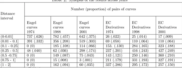
Table 2: Synopsis of the results across years Number (proportion) of pairs of curves Distance
interval
Engel Engel Engel EC EC EC
curves curves curves Derivatives Derivatives Derivatives
1974 1988 2001 1974 1998 2001 (0-0.01] 737 (.626) 782 (.457) 642 (.375) 26 (.022) 25 (.014) 17 (.009) (0.01 - 0.1] 391 (.332) 356 (.208) 519 (.303) 69 (.058) 110 (.064) 110 (.064) (0.1 - 0.25] 0 (0) 185 (.108) 114 (.066) 153. (.130) 284 (.165) 323 (.188) (0.25 - 0.5] 48 (.040) 62 (.036) 298 (.174) 237 (.201) 416 (.243) 427 (.249) (0.5 -0.75] 0 (0) 149 (.087) 75 (.043) 143 (.121) 250 (.146) 360 (.210) (0.75 - 1] 0 (0) 15 (.008) 3 (.001) 211 (.179) 331 (.193) 327 (.191) (1 - 2] 0 (0) 162 (.094) 60 (.035) 337 (.286) 295 (.172) 257 (.150) Note: see note in Table 2.
do not group in few equinumerous clusters or in clusters corresponding to the macro types of expenditures listed in section 2. For any agglomeration criterion used (average, single, complete linkage, Ward) we find that most curves fall into one very large cluster. The other clusters are composed of one or maximum two elements. Specifically, with the average linkage criterion, it emerges a large cluster of ECs consisting of 54 elements when we impose 5 splits. This same cluster contains 53 elements when the splits are six, up to 50 when the splits are ten. The first diagram in Figure 1 displays result from the imposition of 10 splits. Five ECs drawn in a solid line all belong to the same large cluster. The curves in dashed lines are ECs that belong to other, smaller clusters. Curves are readjusted in the y axis so that they can be easily compared by shape. The same analysis is performed for variances and derivatives. Variances group in a manner very similar to ECs. 40 out of the 53 commodity groups fall into one cluster when the sample 8 split are imposed. The second diagram of figure 1 displays both variance curves belonging to the large cluster (solid lines) and variance curves belonging to smaller clusters (dashed lines). Remarkably different results emerge from the analysis of the derivatives. Derivatives exhibit much more heterogeneity in shape, as the third diagram of figure 1 shows. Although a large cluster still emerges, it is smaller relative to the one found in the analysis of simple ECs. More specifically, when 10 splits are imposed the large cluster of derivatives includes 42 commodity groups possessing an average within distance of
d = 0.3311. In contrast, the large cluster of simple ECs contained (for the same number of
splits) 50 commodity groups with average within distance d = 0.0288. Moreover, in the results pertaining to the derivatives, the size of the smaller clusters has also grown, with one cluster containing 6 commodity groups and another with 4 commodity groups.
We also investigate how the distances are distributed in sub-classes of income, dividing the
X axis in three equidistant intervals. In general there is a higher variety of shapes in
sub-classes of income (see table 1, columns 5-7). The most relevant result in this respect is that in the high class of income this heterogeneity dramatically increases. Indeed half of the pairs (50.7%) show a within distance larger than 1. Finally, we repeat our analysis considering two different years: 1974 and 1998. The results are displayed in table 2. The patterns displayed in 2001 emerge to some extent in 1974 and 1998 as well. Kolmogorov-Smirnov tests do not reject similarities in the patterns between 1998 and 2001 (both for ECs and derivatives). However similarities in patterns between 1974 and 1998 are confirmed only as regards EC derivatives and rejected between 1974 and 2001 (both at 0.05 and 0.01 significance level).
5
Discussion and Conclusions
ECs display a very similar shape across different commodities. Noteworthy differences in shapes are observed for only very few expenditure categories. However, a wider variety of shapes emerges when considering derivatives and higher classes of income. When grouping curves (ECs, derivatives or variances) on the basis of their shape, we do not obtain classifi-cations typically made in consumption research. We do, in particular, find no distinction in terms of goods versus services or durable versus non-durable.
The overall dominant EC (see again figure 1) is strictly increasing up to a certain point of
X. Thereafter, we find a class of shapes for which it goes up again, while in others it remains
flat or goes down. This confirms Prais’ (1952) early hypothesis that the “typical shape” of an EC for a commodity g reflects that g has an income elasticity greater than unity at low income levels for which g is a luxury. For higher income levels where g has become a necessity the EC displays an income elasticity between 0 and 1. At a certain level of income expenditure it does not react to increases of income anymore. This is in line with the common assumption that a point of satiety occurs at which the expenditure on g becomes insensitive to further increases in income (Aitchison and Brown 1954, Pasinetti 1981, Witt 2001).
The observed tendency of ECs to change direction at very high levels of X should be cau-tiously interpreted. For this range, there is typically a dramatic decrease in the number of observations. This fact, however, does not bias our results on comparison. This is because the measure incorporated in the rank correlation method weights the sub-intervals of total consumption according to the frequency of observations. Intervals containing few observa-tions thus contribute much less to the overall rank correlation than those which have many observations. How may one now explain the observed heterogeneity of EC derivatives relative to the homogeneity of simple ECs? First, small kinks in the ECs become magnified in the shape of their derivatives. Thus, if an EC has a kink at some level of X and another does not, the respective derivatives of the two curves will differ. Second, the rank correlation method is highly influenced by whether two curves are monotonic over the same intervals. Derivatives of monotonic curves, however, are not necessarily monotonic themselves. Hence, while the rank correlation between two particular ECs may be high, the rank correlation between the derivatives of the same ECs can turn out to be much lower.
In sum, our empirical findings provide new insights into the heterogeneity patterns of consumption behavior. We suggest the following:
1. Some fundamental characteristics of consumption behavior are invariant across expen-diture categories, independently of the sort of commodities involved. These consist of two features as evidenced by the “typical shape” of ECs: (i) families with low income are very sensitive to income increases, and (ii) at a certain level of income a point of satiation is reached.
2. The richer are families, the more various is their consumption behavior. This equally holds across types of expenditures as evidenced by a certain homogeneity in the shape of EC variances. It reflects that households with higher income know less constraints when allocating their budget than poorer households. However, this feature shows less homogeneity across commodities than the characteristics of consumption behaviors. 3. The fact that heterogeneity in consumption behavior becomes higher as income increases
4. Marginal propensities to consume differ in their sensitivity to income across groups of expenditures. This evidenced by the fact that shapes of EC derivatives vary widely across expenditure categories.
References
Aitchison, J. and J.A.C. Brown (1954), A Synthesis of Engel Curve Theory, The Review of Economic Studies, 22(1), 35-46.
Banks, J., R. Blundell, and A. Lewbel (1997), Quadratic Engel Curves and Consumer Demand,
The Review of Economics and Statistics, 79(4), 527-539.
Blundell, R., X. Chen, and D. Kristensen (2007), Semi-Nonparametric IV Estimation of Shape-Invariant Engel Curves, Econometrica, 75(6), 1613-1699.
Engel, J. and A. Kneip (1996), Recent Approaches to Estimating Engel Curves, Journal of
Economics, 63(2), 187-212.
Gasser, T., A. Kneip, and W. K¨ohler (1991), A Flexible and Fast Method for Automatic Smoothing, Journal of the American Statistical Association, 86(14), 643-652.
Gasser, T. and H.G. M¨uller (1984), Estimating Regression Functions and Their Derivatives by the Kernel Method, Scandinavian Journal of Statistics, 11, 171-185.
Gibbons, J.D. (1991), Nonparametric Measures of Association, Newbury Park CA: Sage Pub-lications.
Marron, J.S. and A.B. Tsybakov (1995), Visual Error Criteria for Qualitative Smoothing,
Journal of the American Statistical Association, 90(430), 499-507.
Heckman, N. E. and R. H. Zamar (2000), Comparing the shapes of regression functions,
Biometrika, 87(1), 135-144.
Herrmann, E. (1997), Local Bandwidth Choice in Kernel Regression Estimation, Journal of
Computational and Graphical Statistics, 6(1), 35-54.
Pasinetti, L. (1981), Structural Change and Economic Growth, Cambridge: Cambridge Uni-versity Press.
Prais, S.J. (1952), Non-Linear Estimates of the Engel Curves, The Review of Economic Studies, 20(2), 87-104.
Witt, U. (ed) (2001), Escaping Satiation: The Demand side of economic growth, Springer Verlag, Berlin.