Wealth Effects, the Taylor Rule and the Liquidity Trap
Barbara Annicchiarico Giancarlo Marini Alessandro Piergallini
CEIS Tor Vergata - Research Paper Series, Vol.
35, No.104, May 2007
This paper can be downloaded without charge from the Social Science Research Network Electronic Paper Collection:
http://papers.ssrn.com/paper.taf?abstract_id=986129
CEIS Tor Vergata
R
ESEARCH
P
APER
S
ERIES
Wealth Effects, the Taylor Rule, and the
Liquidity Trap
∗
Barbara Annicchiarico
†University of Rome “Tor Vergata”
Giancarlo Marini
‡University of Rome “Tor Vergata”
Alessandro Piergallini
§CeFiMS, University of London
March 2007
Abstract
This paper analyzes the dynamic properties of the Taylor rule with the zero lower bound on the nominal interest rate in an optimizing monetary model with overlapping generations. The main result is that the presence of wealth effects is not sufficient to rule out the possibility of infinite equilibrium paths with decelerating inflation. In particular, the operation of wealth effects does not avoid the occurrence of liquid-ity traps when the central bank implements a Taylor-type interest-rate feedback rule.
Journal of Economic Literature Classification Numbers: E31, E52. Keywords: Wealth Effects, Taylor Rules, Liquidity Traps.
∗We gratefully acknowledge financial support from the FIRB project.
†Corresponding Author: Department of Economics, University of Rome ‘Tor Vergata’,
Via Columbia 2, 00133 Roma, Italy. E-mail: [email protected]. Phone: +390672595731. Fax: +39062020500.
‡Department of Economics, University of Rome ‘Tor Vergata’, Via Columbia 2, 00133
Roma, Italy. E-mail: [email protected].
§Centre for Financial & Management Studies, University of London, Thornhaugh
1
Introduction
The dynamic effects of Taylor-style policy rules (Taylor, 1993, 1999) have arguably been one of the most debated issues in modern monetary economics. When fiscal solvency is guaranteed, active monetary policies, i.e. interest rate feedback rules increasing the nominal interest rate rule by more than a raise in inflation, have often been proved to induce local rational-expectations equilibrium uniqueness, thus ruling out sunspot fluctuations (e.g., Leeper, 1991; McCallum, 2003; Woodford, 2003). However, it is well known, at least since the seminal contributions by Benhabib, Schmitt-Groh´e and Uribe (2001a, 2001b, 2002), that interest rate rules of Taylor’s type, ensuring the respect of the zero lower bound for the nominal interest rate, are likely to lead to multiple steady-state equilibria and global indeterminacy. In particular, in a dynamic optimizing general equilibrium framework with infinite horizon, Benhabib, Schmitt-Groh´e and Uribe (2001b) demonstrate the existence of an infinite number of equilibrium paths originating around the steady state at which monetary policy is active and converging to a liquidity trap.
The main purpose of the present paper is to investigate whether wealth effects are sufficient to rule out trajectories spiraling down into a liquid-ity trap when the monetary authorities implement Taylor-type interest rate rules. The stabilizing role of wealth effects in preventing the liquidity trap dates back to the seminal works by Pigou (1943, 1947) and Patinkin (1965). However, the implications of wealth effects for the liquidity trap have not been investigated in modern theoretical setups for monetary analysis, that combine dynamic optimizing general equilibrium modeling with monetary
policy rules targeting the short-term nominal interest rate.
In order to rigorously micro-found wealth effects in an optimizing frame-work, we construct a flexible price money-in-the-utility-function version of the Yaari (1965)-Blanchard (1985)-Weil (1989) overlapping generations (olg) setup, extended to the more general case of non-separable preferences. The model we adopt embeds the standard infinitely lived representative agent formulation as a special case and can be usefully employed to consider the issue of global macroeconomic stability under the Taylor rule when wealth effects are operative. In an olg framework `a la Weil (1989), Ireland (2005) shows how the real balance effect is capable of eliminating the liquidity trap when the money supply is the policy instrument. Our model, on the other hand, examines the implications of wealth effects under the assumption that the monetary authority adopts a Taylor rule with the zero bound on nominal interest rates.1
We demonstrate how wealth effects fail to act as automatic stabilizers and can generate an additional source of multiple steady-state equilibria. Our main result is that in the neighborhood of the steady states at which the interest rate feedback rule is active, the operation of wealth effects is not sufficient to avoid multiple perfect-foresight equilibrium trajectories leading the economy to a deflationary trap.
The conventional wisdom that the presence of wealth effects is capable of ruling out the liquidity trap does not hold in a dynamic general equilibrium optimizing framework if the central bank adopts the Taylor rule. Our results
1
In an olg model `a la Weil (1989), B´enassy (2000, 2005) analyzes the issue of price level determinacy under interest rate pegs and a conventional Taylor rule.
thus provide additional theoretical support to the original findings obtained by Benhabib, Schmitt-Groh´e and Uribe (2001b) in the context of the infinite-horizon representative agent paradigm. The possibility of liquidity traps under the Taylor rules is a robust result, which still holds in the presence of wealth effects.
The remainder of the paper is organized as follows. Section 2 presents a monetary model with wealth effects and describes the monetary and the fiscal regimes. Section 3 develops the steady state analysis. Section 4 studies the model equilibrium dynamics and examines the issue of liquidity traps. The concluding Section 5 summarizes the main findings.
2
The Model
The economy is described by a flexible-price monetary version of the Yaari (1965)-Blanchard (1985)-Weil (1989) olg framework. Each individual faces an age-independent instantaneous probability of death, µ > 0. Population is assumed to grow at a constant rate n. At each instant t a new generation is born and the birth rate is defined as β = n + µ.
Let Nt denote population at time t. For analytical convenience,
popula-tion at time t = 0 is normalized to one, N0 = 1. Given the birth rate β and
the death rate µ, the size of the generation born at time t is βNt= βent, while
the size of the surviving cohort born at time s ≤ t is βNse−µ(t−s)= βe−µteβs.
Therefore, total population at time t is Nt= βe−µt
Rt −∞e
βsds.
The economy is characterized by absence of dynastic altruism. Hence, financial wealth of newly born agents is zero. Individuals alive supply one
unit of labor inelastically, which is transformed one-for-one into output. The representative agent of the generation born at time s ≤ 0 chooses the time path of consumption, cs,t, and of real money balances, ms,t, in order
to maximize the following expected lifetime utility function:
E0
Z ∞ 0
log Ω (cs,t, ms,t) e−ρtdt, (1)
where ρ > 0 is the rate of time preference. The sub-utility function, Ω (·), is strictly increasing, strictly concave and linearly homogenous.2 Consumption
and real money balances are Edgeworth complements, hence Ωcm > 0, and
the elasticity of substitution between the two is less than one.3 Individuals
accumulate their financial wealth, as,t, in the form of real money balances and
interest bearing government bonds, bs,t. Let Rt denote the nominal interest
rate, πt the inflation rate and τs,t real lump-sum taxes. Since the probability
at time 0 of being alive at time t ≥ 0 is given by e−µt, equation (1) can be
rewritten as:
Z ∞ 0
log Ω (cs,t, ms,t) e−(µ+ρ)tdt, (2)
The consumer’s instantaneous budget constraint is given by:
•
as,t = (Rt− πt+ µ) as,t+ ys,t− τs,t− cs,t− Rtms,t, (3)
where µas,t is an actuarial fair payment that individuals receive from a
per-2
The assumption of linear homogeneity of the sub-utility function makes aggregation of individual variables across all cohorts analytically tractable.
3
This assumption ensures that money is always essential. See Obstfeld and Rogoff (1983) for details.
fectly competitive life insurance company as long as they survive.4 After
their death, the total amount of their financial wealth accrues to the insur-ance company. In other words, insurinsur-ance companies collect financial assets from deceased members of the population and pay fair premia to surviving individuals (Yaari, 1965). The operation of a life insurance market rules out the possibility for individuals of passing away leaving unintended bequest to their heirs.
The condition precluding agents’ Ponzi-games must also be satisfied:
lim
t→∞as,te
−R0t(Rk−πk)dk ≥ 0. (4)
The individual maximization problem can be solved using a two-stage budgeting procedure. Let zs,t denote total consumption at time t for the
agent born at time s, defined as physical consumption plus the interest for-gone on real money holdings, zs,t = cs,t+Rtms,t. In the first stage, consumers
solve an intra-temporal problem of choosing the optimal allocation between consumption and real money holdings, in order to maximize their instanta-neous utility function, Ω (·), for a given level of total consumption, zs,t. At
the optimum the marginal rate of substitution between consumption and real money holdings is equal to the nominal interest rate:
Ωm(cs,t, ms,t)
Ωc(cs,t, ms,t)
= Rt. (5)
Since preferences are linearly homogenous, the optimal portfolio equilibrium 4
There is uncertainty at the individual level, but not in aggregate. For this reason there is scope for a life insurance market to be operative. See Yaari (1965) for details.
condition (5) is of the form:
cs,t = Γ(Rt)ms,t, (6)
where Γ(·) is such that Γ′(R
t) > 0 and Γ (Rt) − RtΓ′(Rt) > 0.5
In the second stage of maximization, consumers solve the intertemporal problem of deriving the optimal time path of total consumption, zs,t, in order
to maximize their lifetime utility function (2), given the constraints (3), (4) and the optimal condition (6). At the optimum the time path of individual total consumption is (see Appendix B):
•
zs,t= (Rt− πt− ρ) zs,t. (7)
Using the equation of motion of total consumption (7) and condition (6), and recalling that zs,t = cs,t + Rtms,t, one can derive the optimal path of
individual consumption: • cs,t = (Rt− πt− ρ) cs,t− L′(R t) L(Rt) • Rtcs,t, (8)
where L(Rt) ≡ 1 +Γ(RRtt) and L′(Rt) > 0. Note that the optimal consumption
growth rate is the same for all generations. 5
Condition Γ′(R
t) > 0 follows from Ωcc− ΩcmΩc/Ωm< 0 and Ωmm− ΩcmΩm/Ωc< 0;
whereas the sign of Γ (Rt)−RtΓ′(Rt) depends on the the elasticity of substitution between
2.1
Aggregation
The population aggregate for a generic economic variable at individual level, xs,t, is defined as Xt= βe−µt
Rt −∞xs,te
βsds, while the corresponding quantity
in per capita terms is xt= Xte−nt.
Assuming that each agent faces identical age-independent income and tax flows, ys,t = yt and τs,t = τt, for analytical convenience, and recalling
that the wealth of newly born consumers is zero, as,s = 0, we can express
the budget constraint (3) and the optimal time path of consumption in per capita terms (8) as (see Appendix C for details):
• at = (Rt− πt− n) at+ yt− τt− ct− Rtmt, (9) • ct = (Rt− πt− ρ) ct− L′(R t) • Rt L(Rt) ct− β(ρ + µ) L(Rt) at. (10)
The rate of change of per capita consumption depends on the level of finan-cial wealth at. Ricardian equivalence is not verified, since future cohorts’
consumption is not valued by agents alive today. Total government liabili-ties are net wealth for private agents. Older generations are wealthier than younger generations and consume more. Since at each instant of time a new generation is born with no financial wealth, the rate of growth of per capita consumption is lower than individual consumption growth. If the birth rate β were equal to zero, consumption would evolve as in the infinitely-lived representative agent case.
2.2
Monetary and Fiscal Regimes
Following Benhabib, Schmitt-Groh´e and Uribe (2001b), monetary policy is conducted according to an interest rate feedback rule of the form:
Rt= R(πt) ≡ R∗e(A/R
∗)(π
t−π∗), (11)
where π∗ is the target level of inflation, A > 0 and R∗ = π∗+ ρ. Rule (11)
stipulates the impossibility for the monetary authorities to force the nominal interest rate below zero.
Definition 1. An interest rate rule Rt = R(πt) is active (passive) if R′(π
t) > (<)1.
According to Definition 1, the interest rate rule (11) is active (passive) at π∗ if A > (<)1.
The flow budget constraint of the government in per capita terms is:
•
at = (Rt− πt− n) at− τt− Rtmt, (12)
where for expositional simplicity public expenditure is set equal to zero at all times. Taxes are an increasing function of government liabilities adjusted for interest savings on the monetary base, as in Benhabib, Schmitt-Groh´e and Uribe (2001a, 2001b):
τt+ Rtmt= θat, (13)
where θ > 0. This parameter restriction ensures that fiscal policy is “Ricar-dian”, that is, the present discounted value of per-capita total government
liabilities converges to zero for all possible, equilibrium and off-equilibrium, sequences of endogenous variables, namely the price level, the money supply, inflation, and the nominal interest rate:
lim
t→∞ate
−R0t(Rk−πk−n)dk= 0. (14)
To make the implications of our model as much comparable as possible with the results of the standard theory on Taylor rules, we assume θ > R(π∗) −
π∗− n. This parameter restriction is necessary to guarantee that fiscal policy
is “passive” (see Leeper, 1991) or “locally Ricardian” (see Woodford, 2003) around the steady state at which the inflation rate is at its target level, π∗. In
other words, the dynamics of per capital total government liabilities remains bounded for any bounded path of endogenous variables.
2.3
Equilibrium
Total output is assumed to grow at the constant rate n, without loss of generality. It follows that per capita output is constant and can be normalized to one, yt = y = 1, for analytical convenience. Equilibrium in the goods
market requires that ct = y = 1.
Using the equation of motion of per capita consumption (8), we obtain an expression for the equilibrium real interest rate:
Rt− πt= ρ + L′(R t) • Rt L(Rt) + β(ρ + µ) L(Rt) at. (15)
for the inflation rate: • πt= [R(πt) − πt− ρ] L [R(πt)] L′[R(π t)] R′(πt) − β(ρ + µ) L′[R(π t)] R′(πt) at. (16)
Substituting (11) and (13) into (12) gives:
•
at= [R(πt) − πt− n − θ] at. (17)
The initial level of per capita government liabilities a0 must satisfy a0 =
an
0/P0, where an0 is the nominal value of the initial per capita liabilities and
P0 the initial price level.
A perfect-foresight equilibrium of the model can be defined as follows.
Definition 2.A perfect-foresight equilibrium is a set of sequences {πt, at} and an initial price level P0 > 0 satisfying (14), (16) and (17), given an
ini-tial stock of government liabilities, an 0 > 0.
3
Steady State Analysis
Steady state equilibria are defined from equations (16) and (17) setting
•
πt, •
at = 0. In the general case with a positive birth rate and A 6= 1, the
model exhibits four steady-state equilibria.6
Let (π∗, a∗) and (π, a) indicate the pair of steady states characterized
by zero net financial wealth, a∗ = a = 0, and by inflation rates such that
6
The system of equations (16) and (17) displays a degenerate Bogdanov-Takens bifur-cation at A = 1 and θ = ρ − n. See Appendix E for the proof.
R(π∗) − π∗ = R(π) − π = ρ, where π∗ > (<)π if A > (<)1. From equation
(8), at these steady states individual consumption is constant overtime, since the real interest rates, r∗ = R(π∗) − π∗ and r = R(π) − π, are equal to
rate of time preference ρ. The steady states (π∗, a∗) and (π, a) replicate the
equilibrium in which generations are not linked and aggregate consumption is optimally distributed among those alive: each individual only consumes her endowment at all times, so that individual marginal utilities of consumption and real money balances are identical across all generations.
Let (eπ, ea) and (bπ, ba) denote the pair of steady states characterized by inflation rates such that R(eπ) − eπ = R(bπ) − bπ = n + θ and by a pos-itive level of per capita wealth, ea = (n + θ − ρ) L [R(eπ)] /β(µ + ρ) and ba = (n + θ − ρ) L [R(bπ)] /β(µ + ρ), respectively. Let bπ < (>)eπ if A > (<)1. It follows that ba < (>)ea if A > (< 1). At the steady states (eπ, ea) and (bπ, ba), the real interest rates, er = R(eπ) − eπ and br = R(bπ) − bπ, are higher than the rate of time preference ρ. As a result of equation (8), individual consumption is increasing over time, as agents accumulate financial wealth during their life. An asymmetric distribution of aggregate consumption among different generations emerges. Older individuals consume more than the young.
From the interest rate rule (11), using the fact that θ > ρ − n, we can state the following proposition.
Proposition 1. The steady state equilibria of the model (16) and (17) satisfy the following inequalities: eπ > π∗ > π > bπ and ea > ba > 0 if A > 1;
e
4
Dynamic Analysis and Liquidity Traps
We now analyze local and global equilibrium dynamics making use of the following definitions.
Definition 3. The model displays nominal determinacy (indetermi-nacy) around a steady state if for any set of perfect-foresight equilibrium sequences {πt, at}, there exists a unique price level (an infinite number of
initial price levels) P0 > 0 consistent with a perfect-foresight equilibrium.
Definition 4. The model displays real determinacy (indeterminacy) around a steady state if there exists a unique (an infinite) set of perfect-foresight equilibrium sequences {πt, at} converging asymptotically to the steady
state.
Close inspection of (16) and (17) reveals that nominal determinacy occurs because, given an equilibrium sequence of the inflation rate {πt}, evolving
according to equation (16), and an initial level of nominal liabilities, an 0, there
exists a unique price level P0 > 0 consistent with the equilibrium sequence.7
By contrast, in the infinite horizon representative agent setup where β = 0, inflation dynamics do not depend on the time path of real government liabilities. The unique equilibrium sequence {πt} would be consistent with
infinite possible initial price levels and the model would display nominal indeterminacy (see Benhabib, Schmitt-Groh´e and Uribe, 2001a).
Let J(πt,at,) be the Jacobian matrix of the system of equations (16) and
7
This result is consistent with the findings obtained by B´enassy (2005) in the context of an olg monetary model `a la Weil (1989) when monetary policy is conducted according to a conventional Taylor rule.
(17). At the steady states (π∗, a∗), (π, a), (eπ, ea) and (bπ, ba), the Jacobians are, respectively: J(π∗,a∗) = [R ′(π∗) − 1] L[R(π∗)] L′[R(π∗)]R′(π∗) −β (ρ+µ) L′[R(π∗)]R′(π∗) 0 ρ − n − θ , (18) J(π,a) = [R ′(π) − 1] L[R(π)] L′[R(π)]R′(π) −β (ρ+µ) L′[R(π)]R′(π) 0 ρ − n − θ , (19) J(eπ,ea)= [R′(eπ)−1]L[R(eπ)]
L′[R(eπ)]R′(eπ) + [R(eπ) − eπ − ρ] −
β(ρ+µ) L′[R(eπ)]R′(eπ) [R′(eπ) − 1](n+θ−ρ)L[R(eπ)] β(ρ+µ) 0 , (20) J(bπ,ba)= [R′(bπ)−1]L[R(bπ)] L′[R(bπ)]R′(bπ) + [R(bπ) − bπ − ρ] − β(ρ+µ) L′[R(bπ)]R′(bπ) [R′(bπ) − 1](n+θ−ρ)L[R(bπ)] β(ρ+µ) 0 . (21)
In the system of equations (16) and (17), πt is a jump variable and at
is predetermined. Hence the system exhibits a unique convergent solution around a steady state if the real parts of the eigenvalues are of opposite sign (real determinacy), has multiple convergent solutions if the real parts of both eigenvalues are negative (real indeterminacy) and is unstable if they are positive.
Recalling that if A > (<)1, R′(π∗), R′(eπ) > (<)1 and R′(π), R′(bπ) <
Proposition 2. If A > 1, the model displays real determinacy around (π∗, a∗) and (bπ, ba), instability around (eπ, ea) and real indeterminacy around
(π, a).
Proof. If A > 1, the model displays real determinacy around (π∗, a∗) and (bπ, ba), instability around (eπ, ea) and real indeterminacy around (π, a) since det J(π∗,a∗), det J(ba,bπ) < 0 and det J(π,a), det J(ea,eπ) > 0, with trJ(π,a) < 0
and trJ(ea,eπ)> 0. ¥
Proposition 3. If A < 1, the model displays real determinacy around (π, a) and (eπ, ea), instability around (bπ, ba) and real indeterminacy around (π∗, a∗).
Proof. If A < 1, the model displays real determinacy around (π, a) and (eπ, ea), instability around (bπ, ba) and real indeterminacy around (π∗, a∗) since
det J(π,a), det J(ea,eπ) < 0 and det J(ba,bπ), det J(π∗,a∗) > 0, with trJ(ba,bπ) > 0 and
trJ(π∗,a∗)< 0 . ¥
The results stated in Propositions 2 and 3 have the following inter-pretations. At the two steady states (π∗, a∗) and (π, a) characterized by zero
net financial wealth all individuals have the same level of consumption, i.e. there is no intergenerational inequality. Examining the Jacobian matrices (18) and (19), when πt and at remain in a small neighborhood around the
steady states (π∗, a∗) and (π, a), inflation does not affect the dynamics of per
capita real government liabilities, since at (π∗, a∗) and (π, a) ∂a•
t/∂πt = 0,
and hence does not generate redistributions of wealth across generations. In these cases, the determinacy results obtained in the infinitely lived repre-sentative agent setup are replicated. An active monetary policy yields local
equilibrium determinacy. A passive monetary policy causes the equilibrium to be locally indeterminate.
However, there exist two additional steady states, (eπ, ea) and (bπ, ba), with positive non-human wealth. At this pair of steady states individual con-sumption varies across individuals of different generations. Examining the Jacobian matrices (20) and (21), it emerges that in a small neighborhood around the steady states (eπ, ea) and (bπ, ba), inflation does affect real finan-cial wealth dynamics, since at (eπ, ea) ∂a•t/∂πt = [R′(eπ) − 1](n+θ−ρ)L[R(eβ(ρ+µ) π)] 6= 0
and at (bπ, ba) ∂a•t/∂πt = [R′(bπ) − 1](n+θ−ρ)L[R(bβ(ρ+µ) π)] 6= 0, thereby giving rise to
redistributions of wealth across generations. In particular, a positive devia-tion of infladevia-tion from its steady state value produces a redistribudevia-tion of real financial wealth from currently alive private agents to future generations. Inflation decreases the current amount of per capita government liabilities in real terms, thus reducing the need for future fiscal restrictions necessary to guarantee the respect of the public solvency condition. The wealth effect tends to dampen the current value of per capita consumption and there is no need for the central bank to implement a more than proportional increase in the nominal interest rate to ensure equilibrium uniqueness. The determinacy results under interest rate policies break down. Passive monetary policy rules generate local determinacy. Under active monetary policy rules, on the other hand, there is no local perfect-foresight equilibrium in which the sequences {πt, at} converge asymptotically to the steady state.
In order to show how perfect-foresight self-fulfilling deflationary paths characterize global equilibrium dynamics in the presence of wealth effects, we
analysis.
Let the instantaneous utility function be a ces aggregate of consumption and real money balances of the form:
Ω(cs,t, ms,t) =
£
ηcγs,t+ (1 − η)mγs,t¤
1
γ , (22)
where 0 < η < 1 and γ < 0. The elasticity of substitution between con-sumption and real money balances is σ ≡ 1/(1 − γ). It follows that Γ (Rt) =
[η/ (1 − η)]σRσ
t. The model is calibrated under the assumption that each
in-stant of time corresponds to a quarter of year. We set η = 0.94 and σ = 0.39, consistently with the estimates by Chari, Kehoe and McGrattan (2000). We calibrate the instantaneous probability of death at µ = 0.02 and the rate of population growth at n = 0.004. The fiscal parameter θ is set at 0.0015. When monetary policy is active at π∗ the interest rate rule policy parameter
A is set equal to 1.5 (see Taylor, 1993, 1999). We set π∗ = 0.042/4 and
ρ = 0.018/4, as in Benhabib, Schmitt-Groh´e and Uribe (2001b). Table 1 reports the baseline calibration.
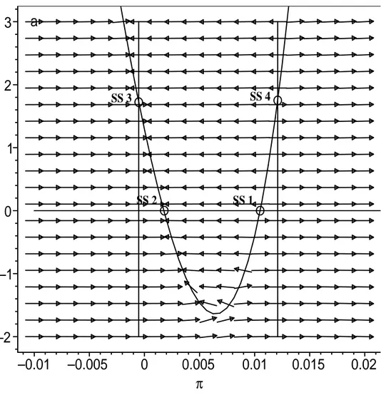
Figure 1 plots the associated phase diagram. The four steady states of our model, (π∗, a∗), (π, a), (eπ, ea), and (bπ, ba), are denoted by SS1, SS2, SS3, and
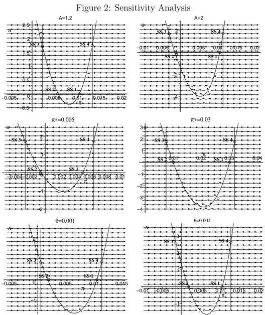
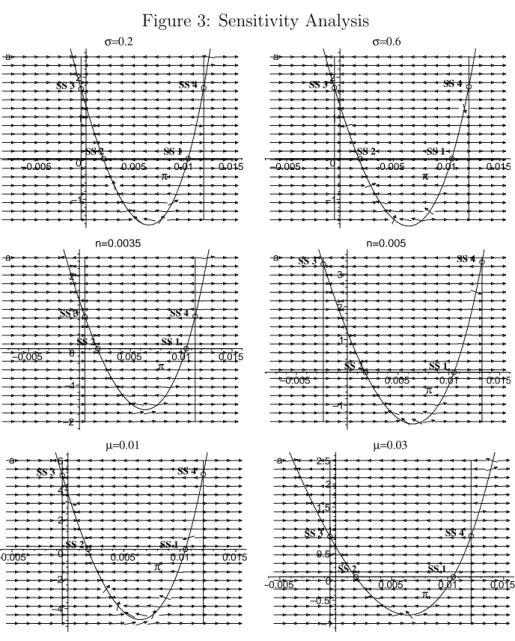
SS4, respectively. The figure reveals the existence of a number of decelerating inflation paths that originate around SS1 and SS4, at which monetary policy is active, and converge either to SS2 or to SS3, at which monetary policy is passive. The decelerating inflation trajectories characterizing the model global dynamics appear to be robust to changes in the baseline parameter values, as shown in Figures 2 and 3.
The economic intuition of our results can be explained as follows. Sup-pose agents expect a decrease in inflation. If the central bank follows the Taylor rule, agents must also expect a decrease in the nominal interest rate. The expected decrease in the opportunity cost of holding money brings about an expected increase in the demand for real balances. According to equation (10), for a given level of current real financial wealth, the expected increase in real balances generates an expected aggregate excess demand for goods. Equilibrium in the goods market requires a fall in the current real interest rate (see equation 15). Since monetary policy is active according to the Tay-lor rule, the decrease in the current real interest rate can occur only if current inflation falls. The decline in inflation is not offset by the presence of wealth effects on aggregate demand since the decrease in the real interest rate has a negative impact on the aggregate accumulation of total real financial wealth (see equation 17), hence amplifying the deflationary pressures over time. Un-der the Taylor rule, the associated self-fulfilling decelerating inflation path is exacerbated by the operation of wealth effects.
5
Conclusions
We have analyzed the role of wealth effects in an general equilibrium model with overlapping generations where the monetary authorities adopt interest-rate feedback rules of the the Taylor-type. Since the original contributions by Pigou (1943, 1947) and Patinkin (1965), wealth effects have been regarded as a channel to avoid the liquidity trap. We demonstrate that this cannel is not at work in our optimizing model. The explicit consideration of these effects
implies the existence of four steady-state equilibria under feedback monetary policy rules, that set the nominal interest rate as an increasing function of inflation, with the zero bound on nominal interest rates. The main conclusion of our analysis is that, also in the presence of wealth effects, the Taylor rule gives rise to an infinite number of perfect-foresight equilibrium paths, in the vicinity of the steady states at which the interest rate rule is active, leading the economy to a liquidity trap.
There are indeed “perils” in adopting Taylor rules, as originally demon-strated by Benhabib, Schmitt-Groh´e and Uribe (2001b). Liquidity traps can occur since the automatic stabilizing role of the Pigou-Patinkin effects is not at work when Taylor rules are implemented.
References
B´enassy, J-P. (2000) ‘Price Level Determinacy under a Pure Interest Rate Peg’, Review of Economic Dynamics 3, 194-211.
B´enassy, J-P. (2005) ‘Interest Rate Rules, Price Determinacy and the Value of Money in a Non-Ricardian World’, Review of Economic Dynamics 8, 651-667.
Benhabib J., S. Schmitt-Groh´e and M. Uribe (2001a), ‘Monetary Policy and Multiple Equilibria’, American Economic Review 91, 167-186.
Benhabib J., S. Schmitt-Groh´e and M. Uribe (2001b), ‘The Perils of Tay-lor Rules’, Journal of Economic Theory 96, 40-69.
Benhabib J., S. Schmitt-Groh´e and M. Uribe (2002), ‘Avoiding Liquidity Traps’, Journal of Political Economy 110, 535-563.
Blanchard, O. J. (1985), ‘Debt, Deficits, and Finite Horizons’, Journal of Political Economy 93, 223-247.
Chari, V.V., P.J. Kehoe and E.R. McGrattan (2000), ‘Sticky Price Mod-els of Business Cycle: Can the Contract Multiplier Solve the Persistence Problem?’, Econometrica 68, 1151-1179.
Ireland, P.N. (2005), ‘The Liquidity Trap, the Real Balances Effect, and the Friedman Rule’, International Economic Review 46, 1271-1301.
Kuznetsov, Y.A. (2004), Elements of Applied Bifurcation Theory, Berlin: Springer-Verlag.
Kuznetsov, Y.A. (2005), ‘Practical Computation of Normal Forms on Center Manifolds at Degenerate Bogdanov-Takens Bifurcation’, International Journal of Bifurcation and Chaos 15, 3535-3546.
Leeper, E. M. (1991), ‘Equilibria under “Active” and “Passive” Monetary and Fiscal Policy’, Journal of Monetary Economics 27, 129-147.
McCallum, B.T (2003), ‘Multiple-Solution Indeterminacies in Monetary Policy Analysis’, Journal of Monetary Economics 50, 1153-1175.
Obstfeld M. and K. Rogoff (1983), ‘Speculative Hyperinflations in Maxi-mizing Models: Can We Rule Them Out?’, Journal of Political Economy 91, 675-687.
Patinkin, D. (1965), Money, Interest, and Prices, New York: Harper and Row (2d Ed.)
Pigou, A.C. (1943), ‘The Classical Stationary State’, The Economic Jour-nal 53, 343-351.
Eco-Taylor, J. B. (1993), ‘Discretion Versus Policy Rules in Practice’, Carnegie-Rochester Conference Series on Public Policy 39, 195-214.
Taylor, J. B. (1999), ‘A Historical Analysis of Monetary Policy Rules’, in J.B.Taylor (Ed.), Monetary Policy Rules, Chicago and London: University of Chicago Press, 319-347.
Weil, P. (1989), ‘Overlapping Families of Infinitely-Lived Agents’, Journal of Public Economics 38, 183-198.
Woodford, M. (2003), Interest and Prices, Princeton and Oxford: Prince-ton University Press.
Yaari, M. E. (1965), ‘Uncertain Lifetime, Life Insurance, and the Theory of the Consumer’, The Review of Economic Studies 32, 137-150.
Yuan, Y. and P. Yu (2003), ‘A Matching Pursuit Technique for Com-puting the Simplest Normal Forms of Vector Fields’, Journal of Symbolic Computation 35, 591-615.
Appendix A
Function Γ(·) is such that Γ′(R
t) > 0 and Γ (Rt) − RtΓ′(Rt) > 0, where the
latter condition follows from the assumption that the elasticity of substitution between consumption and real money balances, σ = d
cs,t ms,t cs,t ms,t /dRt Rt , is less than
one. From (6), in fact:
dcs,t ms,t
= Γ′(Rt) dRt. (23)
Dividing both sides of (23) by cs,t
dcs,t ms,t cs,t ms,t = Γ ′(R t) Γ (Rt) Rt dRt Rt . (24)
It follows that the elasticity of substitution between consumption and real money balances can be expressed as:
σ = d cs,t ms,t cs,t ms,t /dRt Rt = Γ ′(R t) Γ (Rt) Rt. (25)
Appendix B
In the second stage of the individual optimization problem, the representative consumer born at time s solves an intertemporal optimization problem and derives the optimal time path of total consumption, zs,t, to maximize the
lifetime utility function (2), given (6) and the constraints (3) and (4). Using the definition of total consumption, zs,t= cs,t+Rtms,t, and the optimal
intra-temporal condition (6), the instantaneous utility function can be expressed in function of total consumption:
log Ω (cs,t, ms,t) = log qt+ log zs,t, (26)
where qt≡ Ω ³ Γ(Rt) Γ(Rt)+Rt, 1 Γ(Rt)+Rt ´
can be interpreted as the utility-based cost of living index of the basket of physical goods and real balances.
Using this result, the intertemporal optimization problem can be stated as follows: max {zs,t} Z ∞ 0 (log qt+ log zs,t) e−(µ+ρ)tdt, (27)
subject to
•
as,t = (Rt− πt+ µ) as,t+ ys,t− τs,t− zs,t, (28)
and given as,t.
The optimal solution yields the Euler equation characterizing the optimal path of total consumption for an individual:
•
zs,t = (Rt− πt− ρ)zs,t. (29)
Integrating forward the instantaneous budget constraint (28), given the transver-sality condition (4), and using (29) we can formulate total consumption as a linear function of total wealth:
zs,t = (µ + ρ)
¡
as,t+ hs,t
¢
, (30)
where hs,t is human wealth, defined as the present discounted value of
after-tax labor income, hs,t =
R∞ t ¡ ys,v− τs,v ¢ e−Rtv(Rk−πk+µ)dkdv.
Using the definition of total consumption and recalling (6) give:
zs,t= L(Rt)cs,t, (31) where L(Rt) = 1 +Γ(RRtt) with L′(Rt) = Γ(Rt)−RtΓ ′(R t) [Γ(Rt)]2 . Time-differentiating (31) yields: • zs,t = L′(Rt)cs,t • Rt+ L(Rt) • cs,t. (32)
dy-namic equation for individual consumption: • cs,t = (Rt− πt− ρ) cs,t− L′(R t) • Rt L(Rt) cs,t. (33)
This shows equation (8).
Appendix C
By definition, per capita aggregate financial wealth is:
at = β
Z t −∞
as,teβ(s−t)ds. (34)
Differentiating with respect to time the above equation using Leibnitz’s rule, one obtains: • at= βat,t− βat+ β Z t −∞ • as,teβ(s−t)ds, (35)
where βat,tis the newborns’ financial wealth and is equal to zero by
assump-tion (agents are born with zero wealth since there is no bequest motive). Using (3), (35) can be re-written as:
•
at = −βat+ µat+ (Rt− πt) at+ yt− τt− ct− Rtmt (36)
= (Rt− πt− n) at+ yt− τt− ct− Rtmt.
This shows (9).
the individual consumption function is obtained as: cs,t= µ + ρ L(Rt) ¡ as,t+ hs,t ¢ . (37)
The per capita consumption is thus given by:
ct= µ + ρ L(Rt) (at+ ht) , (38) where ht = R∞ t (yv− τv) e− Rv
t(Rk−πk+µ)dkdv. Differentiating with respect
to time the definition of per capita consumption, ct = βe−βt
Rt −∞cs,teβsds, yields: • ct= βct,t− βct+ β Z t −∞ • cs,teβ(s−t)ds, (39)
where the term βct,t denotes consumption of the newborn generation and is
equal to βct,t = β(µ + ρ)ht/L(Rt). Using (8) and (38) into (39) results in the
following time path of consumption per unit of labor:
• ct = (Rt− πt− ρ) ct− L′(R t) • Rt L(Rt) ct− β(ρ + µ) L(Rt) at. (40) This shows (10).
Appendix D
In order to translate the interior equilibrium to the origin and simplify no-tation, we set ιt ≡ πt− π∗ and ℓt ≡ −Lβ(ρ+µ)′(R∗)Aat. The model (16)-(17) given
the Taylor rule (11) can be re-written as: • ιt = £ R∗e(A/R∗)xt − ι t− π∗− ρ ¤ L£R∗e(A/R∗)ιt¤ L′[R∗e(A/R∗)ιt ] Ae(A/R∗)ιt + (41) + L ′(R∗) A L′[R∗e(A/R∗)ιt ] Ae(A/R∗)ιtℓt • ℓt= £ R∗e(A/R∗)ιt − ι t− π∗− n − θ ¤ L′(R∗) A β(ρ + µ)ℓt (42)
At (0, 0), for A = 1 and θ = ρ − n, there is a double zero eigenvalue. In fact, the Jordan block is of the form:
J = 0 1 0 0 , (43)
which is a necessary condition for a Bogdanov-Takens bifurcation.
The bifurcation scenario near the Bogdanov-Takens point depends on the coefficients of the critical normal form on the two-dimensional center manifold which is of the form (Kuznetsov, 2004, 2005):
• u1 = u2, (44) • u2 = X k≥2 ¡ akuk1 + bkuk−11 u2 ¢ . (45)
In order to compute the simplest normal form of this Bogdanov-Takens sin-gularity, we use the matching pursuit technique proposed by Yu and Yuan (2003) under the assumption that the sub-utility function is of the form
Ω(cs,t, ms,t) =
£
ηcγs,t+ (1 − η)mγs,t¤1/γ. We get the following result:
• u1 = u2, (46) • u2 = b1u1u2+ b2u21u2+ a4u41, (47) where b1 ≡ π∗+³ η 1−η ´σ (π∗+ ρ)σ + ρ (π∗+ ρ) (1 − σ) , b2 ≡ (π∗+ ρ)σ³ η 1−η ´σ (3σ − 2) + (2 − σ) (π∗+ ρ) 2 (π∗+ ρ)2(1 − σ) , a4 ≡ − 1 4 π∗+³ η 1−η ´σ (π∗+ ρ)σ + ρ (π∗+ ρ)2(1 − σ) .
Since a2 = 0, the Bogdanov-Takens bifurcation at (0, 0) for A = 1 and
Table 1: Baseline Calibration
Rate of population growth n 0.004
Probability of death µ 0.02
Rate of time preference ρ 0.018/4
Elasticity of substitution between consumption and real money balances σ 0.39
Weight of consumption in the utility function η 0.94
Monetary policy parameter A 1.5
Fiscal rule parameter θ 0.0015
Figure 1: Phase Diagram under the Baseline Calibration SS 3 SS 1
a
SS 2 SS 4–2
–1
0
1
2
3
–0.01
–0.005
0
0.005
0.01
0.015
0.02
π
Figure 2: Sensitivity Analysis A=1.2 a SS 2 SS 4 SS 1 SS 3 –0.5 0 0.5 1 1.5 2 2.5 –0.005 0.005 0.01 0.015 0.02 π A=2 a SS 1 SS 4 SS 3 SS 2 –4 –2 0 2 –0.01 –0.005 0.005 0.01π 0.015 0.02 π∗=0.005 SS 2 a SS 4 SS 3 SS 1 –2 –1 0 1 2 –0.004–0.002 0.002 0.004 0.006 0.008 0.01 π π∗=0.03 SS 1 SS 4 SS 3 SS 2 a –4 –3 –2 –1 1 2 3 0.01 0.02π 0.03 0.04 θ=0.001 SS 2 a SS 4 SS 1 SS 3 –1 0 1 2 –0.005 0.005 0.01 0.015 π θ=0.002 a SS 4 SS 3 SS 1 SS 2 –1 1 2 3 –0.01 –0.005 0.005 0.01 0.015 0.02 π
Figure 3: Sensitivity Analysis σ=0.2 SS 2 a SS 4 SS 3 SS 1 –1 0 1 2 –0.005 0.005 0.01 0.015 π σ=0.6 SS 2 a SS 3 SS 1 SS 4 –1 0 1 2 –0.005 0.005 0.01 0.015 π n=0.0035 a SS 3 SS 2 SS 1 SS 4 –2 –1 0 1 2 –0.005 0.005 0.01 0.015 π n=0.005 SS 2 a SS 1 SS 4 SS 3 –1 1 2 3 –0.005 0.005 0.01 0.015 π µ=0.01 a SS 2 SS 4 SS 3 SS 1 –4 –2 0 2 4 6 –0.005 0.005 0.01 0.015 π µ=0.03 SS 3 a SS 2 SS 1 SS 4 –1 –0.5 0 0.5 1 1.5 2 2.5 –0.005 0.005 0.01 0.015 π