3GPP LTE-Advanced, the evolution of LTE release 8, represents the next gen-eration technology for wireless mobile networks. Wireless backhauling, whereby usually smaller cells use the wireless links as a coordinated backhaul technol-ogy in lieu of wired connection, is one of the key technoltechnol-ogy enhancements in LTE-Advanced to fulfill the performance requirements and to improve the user experience.
Two modes have been envisaged for this technology: the in-band mode, considered in most studies, is the focus of the current 3GPP LTE-Advanced specification. In the latter, transmission to cellular users take place using the same resources as backhauling. However, with evolution of cellular systems, a multi-carrier option is expected to be available. This enables implementation of the out-band operation mode, in an operator controlled spectrum, accord-ing to which the time/frequency resources used for cellular transmission and backhauling are separate.
In any case, backhauling transmissions must be scheduled in order to avoid interference. In this work, we present an energy-efficient link scheduler for out-of-band multi-hop wireless backhauling, with three objectives: first, to be able to carry a required load at each node. Second, to reduce the power consumed by the nodes during transmission and enable coverage extension. Third, to increase network reliability by allowing for fast rerouting of traffic demands in case of a node/link failure. We study the problem from three complementary points of view: the planning one, for which we provide tools that allow a planner to compute worst-case link quality given the phyisical layout of the network. second, the (long-term) link-scheduling one, for which we provide an optimal algorithm to route demands that keeps into account power consumption and avoids unreliable nodes as much as possible. Third, we propose a recovery algorithm that is able to reroute demands in the presence of a failure, at a lower computation cost than recomputing the whole link schedule.
Contents
1 Introduction 8
1.1 Evolution of mobile systems . . . 8
1.2 Backhauling problem . . . 9
1.3 Thesis contributions . . . 9
1.4 Organization of this thesis . . . 10
2 Background 11 2.1 LTE Technology . . . 11
2.1.1 LTE Targets . . . 11
2.1.2 System Architecture . . . 11
2.1.3 Physical Resources . . . 12
2.2 The Heterogeneous Network . . . 13
2.3 Wireless Mesh Network Architecture . . . 14
2.4 Mobile Backhaul . . . 15
2.4.1 Mobile Backhaul overview . . . 15
2.4.2 Backhaul connections . . . 15
2.5 Power Model . . . 16
2.6 CPLEX . . . 18
2.6.1 What is CPLEX . . . 18
2.6.2 Callable Library Component . . . 19
2.6.3 Example of use . . . 20
2.7 Related work . . . 22
2.7.1 Relay . . . 22
2.7.2 Backhauling . . . 23
2.7.3 Critical review . . . 23
3 System model and problem formulation 24 3.1 Problem description . . . 24 3.2 Problem division . . . 25 3.3 Software Implementation . . . 26 4 Node Deployment 27 4.1 Target . . . 27 4.2 Grid Deployment . . . 27 4.3 Random Deployment . . . 27 4.4 Configuration Deployment . . . 28
5 Network Planning 30
5.1 Problem Description . . . 30
5.2 Connectivity Graph . . . 30
5.3 Conflict Graph . . . 31
5.4 Worst-Case CQI computing . . . 31
5.4.1 Problem Formulation . . . 32
6 Routing and Link scheduling power efficient algorithm 34 6.1 Problem description . . . 34
6.2 Formulation of the power efficient link scheduling algorithm . . . 35
7 Recovery Problem 39 7.1 Problem Description . . . 39 7.2 Problem Formulation . . . 42 8 Performance evaluation 45 8.1 Scenario . . . 45 8.1.1 Grid Scenario . . . 45 8.1.2 Ring Scenario . . . 45 8.1.3 Baseline . . . 45 8.2 Preliminary Assumption . . . 45 8.3 Grid Scenario . . . 49 8.3.1 Baseline . . . 49 8.3.2 Scenario Set-up . . . 50 8.3.3 Scenario Evaluation . . . 54 8.4 Ring Scenario . . . 61 8.4.1 Baseline Ring . . . 61 8.4.2 Scenario Set-up . . . 62 8.4.3 Scenario Evaluation . . . 66 9 Conclusion 72 10 Acknowledgement 73
List of Figures
2.1 LTE Evolved Packet System . . . 122.2 LTE time-frequency resource . . . 13
2.3 Heterogeneus network . . . 14
2.4 Heterogeneous and Wireless Mesh Network . . . 15
2.6 View of the Callable Library . . . 20 3.1 Hyperframe . . . 24 3.2 Hyperframe Vector . . . 25 3.3 Problem Division . . . 25 4.1 Grid Deployment . . . 28 4.2 Random Deployment . . . 29
5.1 Example of Connectivity Graph . . . 30
5.2 Logical connectivity graph (left) and conflict graph (right) of a Wireless Mesh Network (WMN) . . . 32
5.3 Worst Case Graph . . . 32
6.1 Relevant quantities in link scheduling . . . 34
6.2 Simple flow’s path . . . 35
6.3 Worst-case delay . . . 35
6.4 Overlapping Flows . . . 37
6.5 Flow Conservation . . . 38
6.6 Resource Allocation . . . 38
7.1 Example Network . . . 39
7.2 Example Network after the failure . . . 40
7.3 Network during node failure . . . 40
7.4 Network’s path after recovery phase . . . 40
7.5 Resource allocation before (a) and after (b) node failure . . . 41
7.6 Resource Block indexes during recovery phase . . . 44
8.1 Node Deployment Example . . . 46
8.2 Node Deployment Example: Edge Number trend . . . 47
8.3 Node Deployment Example - Edge Number trend . . . 48
8.4 Grid Baseline : Connectivity Fulfilled . . . 49
8.5 Grid Baseline : Average Bit-Rate Trend . . . 50
8.6 Grid Scenario . . . 51
8.7 Grid Scenario - Average bit-rate trend . . . 51
8.8 Grid Scenario - Step Configurations . . . 53
8.9 Grid Scenario - Step Configurations Comparison : PLH . . . 53
8.10 Grid Scenario - Number of Conflict Comparison : PLH . . . 54
8.11 Grid Scenario - Simultaneous Transmissions: PLH . . . 54
8.12 Grid Scenario - Step Configurations Comparison : PLL . . . 55
8.13 Grid Scenario - Number of Conflict Comparison : PLL . . . 55
8.14 Grid Scenario - Simultaneous Transmissions: PLL . . . 56
8.15 Grid Scenario - Uplink Traffic Load Managed . . . 57
8.16 Grid Scenario - Uplink Power Consumed . . . 57
8.17 Grid Scenario - Uplink RBs Usage . . . 58
8.19 Grid Scenario - Downlink Power Consumed . . . 60
8.20 Grid Scenario - Downlink RBs Usage . . . 60
8.21 Ring Baseline - Connectivity Fulfilled . . . 61
8.22 Ring Baseline - Average Bit-Rate Trend . . . 62
8.23 Ring Scenario . . . 62
8.24 Ring Scenario - Average bit-rate trend . . . 63
8.25 Ring Scenario - Step Configurations . . . 64
8.26 Ring Scenario - Step Configurations Comparison : PLH . . . 65
8.27 Ring Scenario - Number of Conflict Comparison : PLH . . . 65
8.28 Ring Scenario - Simultaneous Transmissions : PLH . . . 66
8.29 Ring Scenario - Step Configurations Comparison : PLL . . . 66
8.30 Ring Scenario - Number of Conflict Comparison : PLL . . . 67
8.31 Ring Scenario - Simultaneous Transmissions : PLL . . . 67
8.32 Ring Scenario - Uplink Traffic Load Managed . . . 68
8.33 Ring Scenario - Uplink Power Consumed . . . 69
8.34 Ring Scenario - Uplink RBs Usage . . . 69
8.35 Ring Scenario - Downlink Traffic Load Managed . . . 70
8.36 Ring Scenario - Downlink Power Consumed . . . 70
8.37 Ring Scenario - Downlink RBs Usage . . . 71
List of Tables
2.1 Power consumption parameter . . . 162.2 Power Model parameter . . . 17
2.3 Power Model parameters . . . 18
4.1 Example of micro antenna configuration in grid deployment . . . 27
4.2 Example of macro antenna configuration in grid deployment . . . 28
4.3 Example of parameter settings in random deployment . . . 29
5.1 Example of CQI interference . . . 31
8.1 Micro Node Settings . . . 46
8.2 Macro Node Settings . . . 46
8.3 Grid Baseline - Node Settings . . . 50
8.4 Grid Scenario - Micro Node Settings . . . 50
8.5 Grid Scenario - Distance threshold . . . 52
8.6 Grid Scenario - Power Level . . . 52
8.7 Grid Scenario - Settings . . . 54
8.8 Grid Scenario - Simulation parameters . . . 56
8.9 Ring Baseline - Node Settings . . . 61
8.10 Ring Scenario - Micro Node Settings . . . 63
8.12 Ring Scenario - Power Level . . . 64 8.13 Ring Scenario - Settings . . . 65 8.14 Ring Scenario - Simulation parameters . . . 68
Acronyms
3GPP Third Generation Partnership Project CQI Channel Quality Index
DF Decode and Forward eNb Evolved NodeB EPC Evolved Packet Core
E-UTRAN Evolved UMTS Terrestrial Radio Access Network HetNet Heterogeneous Network
HSPA High Speed Packet Access LOS Line Of Sight
LP Linear Programming LTE Long Term Evolution LTE-A LTE-Advanced
MIMO Multiple Input Multiple Output MIP Mixed Integer Programming MME Mobility Management Entity
OFDM Orthogonal Frequency Division Multiplexing POP Point of Presence
RB Resource Block
SAE System Architecture Evolution
SAE-GW System Architecture Evolution Gateway TDMA Time Division Multiple Access
TTI Transmission Time Interval UE User Equipment
WCD Worst Case Delay WMN Wireless Mesh Network
1
Introduction
The first chapter describes the evolution of the mobile systems technology and the reasons that led to the development of the next generation wireless networks are presented.
In section 1.1 a description of the evolution of mobile systems up to the development of LTE-Advanced (LTE-A).
In section 1.2 the backahuling problem is discussed, in section 1.3 the con-tributions of this thesis are given.
The organization of this thesis end the chapter, in section 1.4.
1.1
Evolution of mobile systems
Mobile communications have become an everyday commodity. In the last decades, they have evolved from being an expensive technology for a few selected individ-uals to today’s ubiquitous systems used by a majority of the world’s population. The task of developing mobile technologies has also changed, from being a national or regional concern to becoming an increasingly complex task under-taken by global standard-developing organizations such as the Third Generation Partnership Project (3GPP) [1] and involving thousand of people.
Mobile communication technologies are often divided into generations, with 1G being the analog mobile radio systems of the 1980s, 2G the first digital mobile systems, and 3G the first mobile systems handling broadband data.
The recent increase of mobile data usage and emergence of new applications such as Mobile TV, Web 2.0 and Streaming Video have motivated the 3GPP to work on the next generation of wireless technology called Long Term Evolution (LTE).
The LTE [2] and LTE-A [3] releases are the most important step towards the development of the fourth generation (4G) system.
3GPP has been working on various aspects to improve LTE performance which includes higher order Multiple Input Multiple Output (MIMO), carrier aggregation and heterogeneous networks. The improvements in spectral effi-ciency per link is approaching theoretical limits with 3G and LTE, the next generation of technology is about improving spectral efficiency per unit area.
LTE-Advanced needs to provide an uniform user experience to users any-where inside a cell by changing the topology of traditional networks. A key aspect of LTE-Advanced is about this new deployment strategy using Hetero-geneous Network that implies the use of multiple types of antennas to provide wide area coverage.
The heterogeneous cellular system consists of placement of macro base-station that typically transmits at high power level, overlaid with several micro
base-stations, femto base-station and relay base-stations, which transmits at lower power levels.
Small cells are primarily added to increase capacity in hot-spots with high user demand and to fill in areas not covered by the macro network. They also improve network performance and service quality by offloading from the large macro-cells. The result is a heterogeneous network with large macro-cells in combination with small-cell providing increased bit-rates per unit area.
1.2
Backhauling problem
With the increasing number of smaller base station sites, backhauling these connections to nearest operator Point of Presence (POP) will eventually become problematic. The fiber infrastructure used in aggregation and core transport is not always feasible extended due to the cost and the location accessibility. One way to backhaul the sites is to use wireless links due to their flexibility and their installation cost.
Backhaul link can either be in-band or out-band. The former case, treated in most of the studies, operate in the same spectrum as communication from/to mobile terminals. The use of the same resources lead to a reduction of those used by the user worsening the user-experience. Accordingly to the above statement and with evolution of cellular systems, a multi-carrier option is expected to be available. This enable the implementation of the out-band backhauling where the time/frequency resources used for cellular transmission and backhauling are separate.
1.3
Thesis contributions
As seen in previous section the backhauling and its link-scheduling it’s become challenging and it’s assuming more importance with the increasing number of smaller base station used in the LTE-A network deployment. This work ap-proach the problem of resource allocation of backhauling traffic taking account of the following aspects:
• Energy-efficiency • Flows’ delay • Network reliability
The idea is to use multi-hopping among the antennas to schedule the back-haul traffic.
Backhauling transmissions must be scheduled in order to avoid interference. This thesis approach the backhaul traffic resource allocation
1.4
Organization of this thesis
A review of the LTE technology and a detailed explanation of the main concept studied in the thesis is given in Chapter 2. Chapter 3 presents an overall view of the system. In Chapters 4, 5, 6 and in 7 the designed system is explained in each part. In Chapter 8 performance evaluation of the proposed system is given. Chapter 9 ends the thesis.
2
Background
In this chapter an overview of the LTE is given to better understand the analysis made in the following sections.
In section 2.1 the major concepts related to LTE are described. Section 2.2 presents the concept of heterogeneous network. In section 2.4 we will give a detailed description of the Mobile Backhaul
2.1
LTE Technology
2.1.1 LTE Targets
The work towards 3GPP LTE started in 2004 with the definition of the targets. It takes more than 5 years from setting the system targets to commercial de-ployment using interoperable standards. A few driving forces can be identified advancing LTE development: wireline capability evolution, the need for addi-tional wireless capacity, the need for lower cost wireless data delivery and the competition of other wireless technologies.
LTE must be able to deliver superior performance compared to existing 3GPP networks based on High Speed Packet Access (HSPA) technology. The performance targets in 3GPP are defined relative to HSPA in Release 6. The main performance targets are listed below :
• spectral efficiency two to four times more than with HSPA Release 6 • peak rates exceed 100 Mbps in downlink and 50 Mbps in uplink • enables round trip time lower than 10 ms
• packet switched optimized
• high level of mobility and security • optimized terminal power efficiency
• frequency flexibility with from below 1.5 MHz up to 20 MHz allocations
2.1.2 System Architecture
The system architecture of LTE is based on 3GPP System Architecture Evolu-tion (SAE) and is designed aiming to optimize packet switched services, high data rates and low packet delivery delays.
The architecture is divided into three main levels (Figure 2.1 ). Our work is focused on two of them, User Equipment and Evolved UMTS Terrestrial Radio Access Network (E-UTRAN). A detailed explanation about LTE SAE can be found in [4].
Figure 2.1: LTE Evolved Packet System
User Equipment (UE) is the device that the end user uses for communication. Functionally the UE is a platform for communication applications,which signal with the network for setting up, maintaining and removing the communication links the end user needs.
The E-UTRAN part is composed by the Evolved NodeB (eNb). Nodes are connected through a wired link to the Evolved Packet Core (EPC) network using S1 interface and are connected each other using the X2 interface.
The eNb is a radio base station that is in control off all radio related func-tions in the fixed part of the system. Base station such as eNb are distributed throughout the networks coverage area, each eNb resides near the actual ra-dio antennas. eNb acts as a layer 2 bridge between UE and EPC, by being the termination point of all the radio protocols towards the UE, and relaying data between the radio connection and the corresponding IP based connectivity towards the core network.
The EPC comprises the Mobility Management Entity (MME) and the
Sys-tem Architecture Evolution Gateway (SAE-GW). The former take cares of
authentication and security, subscription and service connectivity and mobility. The latter, instead, is responsible of data forwarding.
2.1.3 Physical Resources
LTE uses Orthogonal Frequency Division Multiplexing (OFDM) as basic trans-mission scheme for both uplink and downlink transtrans-mission. OFDM carries out the same functions as any other multiple access technique, by allowing the base station to communicate with several different mobiles at the same time.
Transmitter divides the information into several parallel sub-streams, and send each sub-stream on a different frequency known as a sub-carrier with a spacing equal to 15 KHz for both downlink and uplink.
In time domain, LTE transmissions are organized into frames of length 10ms, each of which is divided into ten subframes of length 1ms. Each subframe
consists of two equally sized slots of length 0.5ms, with each slot consisting of 6/7 OFDM symbols.
A resource element, consisting of one sub-carrier during one OFDM sym-bol, is the smallest physical resource in LTE. Furthermore, resource elements are grouped into resource blocks, where each resource block consists of 12 con-secutive sub-carriers in the frequency domain and one 0.5 ms slot in the time domain.
Although resource blocks are defined over one slot, the basic time-domain unit for dynamic scheduling in LTE is one subframe, consisting of two consec-utive slots : this 1ms time is called Transmission Time Interval (TTI). The overall time-frequency structure is depicted in Figure 2.2.
Figure 2.2: LTE time-frequency resource
2.2
The Heterogeneous Network
In the past years mobile data traffics has grown exponentially, to battle this expansion LTE-Advanced introduced the concept of heterogeneous network de-ployments along its antenna and radio interface specific addition. With het-erogeneous networks, a coverage area of a macro-node is enhanced by adding base stations with shorter coverage to handle some of the traffic of the macro-nodes. Small cells are primarily added to increase capacity in hot-spots with high user demand and to fill in areas not covered by the macro network. They also improve network performance and service quality by offloading from the large macro-cells.
Figure 2.3 shows the heterogeneus’ network deployment in a singular cell. The result is a heterogeneous network with large macro-cells in combination with small-cell providing increased bit-rates per unit area. Small cells are connected to the Macro with a one hop wired or wireless link. Cell contains two type of node : macro-node and micro-node, in the downlink period macro-node are the traffic source and in the uplink period are the destinations.
of-Figure 2.3: Heterogeneus network
floaded to the micro-node improving the overall system performance. Micro-node are used to improve the performance of the UE near the cell edge, the deployment of micro-node near cell edge or where the traffic demand is high improve the capacity of the network and the throughput fairness over the cell. Micro-node can be also used to provide more Line Of Sight (LOS) connection. In the urban deployment, for example, micro-node are placed in unusual loca-tion like lamp posts, bridges and building walls. Wired backhaul is not always feasible in this kind of deployment so wireless connections become more attrac-tive. Wireless connection are also cheaper and easier to install than the wired connection.
The heterogeneous network are characterized by one-hop connections be-tween Macro and Micro nodes. Connections can be improved to obtain a WMN as explained in the following section.
2.3
Wireless Mesh Network Architecture
WMN consists of stationary wireless routers interconnected by wireless links with a small fraction acting as gateways to the Internet via wired or wireless links. WMNs can provide broadband access in remote area or difficult-to-wire areas keeping the cost-efficiency. Moreover WMN provide larger cover area, lower costs of backhaul connections and ensure alternative paths in case of node failure.
The WMN deployment impose to solve the problem of interference among wireless links, interference can be treated either in frequency or time domain. In the former case different frequencies are assigned to interfering links, the latter assign to each link the full spectrum but interfering links are separated in time domain (Time Division Multiple Access (TDMA)). In case of frequency division it’s necessary to solve a problem of channel assignment, in time-domain the time is slotted and a link scheduling problem activates the non-interfering
links in the same time slot.
Figure 2.4: Heterogeneous and Wireless Mesh Network
As we can see in Figure 2.4 WMN has more edges compared to the Hetero-geneous Network solution. WMN deployment introduce the possibility to have more that one possibly path but also introduce more point-of-failure. The above characteristic are challenging during the WMN resource allocation.
2.4
Mobile Backhaul
The transport infrastructure between a radio access network and a core network is called the mobile backhaul. The basic function of mobile backhaul is to pro-vide transparent connectivity service between base stations and core controllers. Along with LTE- Advanced and heterogeneous networks, the backhaul design has proven challenging.
This section present the concept of mobile backhauling. In section 2.4.1 the basic functionalities of mobile backhauling are discussed. In section
2.4.1 Mobile Backhaul overview
The mobile network architecture illustrations presented in section give a rather high-level logical view on how the elements of a mobile network are intercon-nected. The interconnecting network between the access network and the EPC is the mobile backhaul transport network. Thus, the mobile backhaul connects a large number of eNb sites to a small amount of centralized control sites.
The mobile traffic growth inevitably affect the backhaul, its designing and its implementation need to evolve accordingly. Mobile backhaul need to give more support to mobile networks in term of resiliency, quality and cost-efficiency.
2.4.2 Backhaul connections
Mobile backhauling can be sorted out using different type of connections and resources. The available connections are wired or wireless. The former solution is to provide a wired connections to each base stations. This solution provide a
communication with low interference but introduce a high installation cost due to the wiring of each antenna. Furthermore provide a wired connections to each antennas is not always possible.
Wireless solution is cost-efficient and it’s always feasible even in difficult-to-wire areas. This solution implies a higher level of interference due to the difficult-to-wireless links, as seen in 2.3 this problem can be face in two different manner: time or frequency.
2.5
Power Model
One goal of the performance and evaluation phase is to establish the range of convenience of multi- hop and mesh solutions against one hop solution, to achieve this result we need to calculate the power used to transmit a resource block depending on the transmission power. In [5] and [6] the site’s power consumption in case of maximum load is modelled as follows:
PiM AX = ai∗ Ptx+ bi (2.1)
where,
PiM AX = consumed power in case of maximum load Pi = average consumed power
Ptx = average radiated power
ai = accounts for power consumption that scales with the average
radiated power due to amplifier and feeder losses as well as cooling of sites bi = models an offset of site power which is consumed independently
of the average transmit power due to signal processing The parameters’ value are summarized in 2.1 ([6]).
Base station type ai bi
Macro 21.45 354.44
Micro 5.5 38
Table 2.1: Power consumption parameter
In [6] the backhaul contribution is modelled like a step function. Two power regions(Plow−c andPhigh−c ) for each base station were defined, one for low
capacity traffic conditions and the other for high traffic capacity conditions. The backhaul traffic model presented in [6] doesnt take account of the number
of resource blocks used in the backhaul and result less accurate than the one presented as follows [7] and represented in Figure 2.5:
Pi0 = Pbase+ N ∗ Pin (2.2)
where,
Pin= power consumed to transmit one RB
Pbase = power consumed to turn on the antenna RB
N = number of blocks used in case of maximum load
Figure 2.5: Power Model
The parameters setting of the model presented in [7] are summarized in 2.2 Base station type Pin(W ) Ptx(dBm) Pbase(W ) N
Macro 2.51 40 320 100
Micro 0.450 30 16 100
Table 2.2: Power Model parameter
Considering the maximum load in the two presented models we can set the equality between equations 2.2 and 2.1. We obtain the following equation:
N ∗ Pin= ai∗ Ptx+ bi (2.3)
Using equation 2.3 and the relationship between ai and bi, given by data of
Table 2.1, we can define the problem as follows:
N ∗ Pin= ai∗ Ptx+ bi (2.4)
After solving equation 2.4 and 2.5 we obtain the parameters ai and bi : N ∗ Pin= ai∗ Ptx+ 16.524 ∗ ai ai= N ∗ Pin Ptx+ 16.524 = 4.44 bi= 16.524 ∗ ai= 73.367
We apply the power model reported in 2.4 and 2.5 to the micro and the macro antenna obtaining the parameters reported in Table 2.3 :
Base station type Pbase(W ) ai bi
Macro 320 4.44 73.367
Micro 16 1.22 8.430
Table 2.3: Power Model parameters
Using the parameters reported in Table 2.3 we define the consumed power to transmit a RB by a Macro (PM
in) and by a Micro (PinN) depending on the
transmission power as follows:
PinM = aMi ∗ PM tx + b M i (2.6) PinN = aNi ∗ PN tx + b N i (2.7)
2.6
CPLEX
In this section, we describe IBM ILOGR CPLEXR [8] [9], the tool usedR
to solve the mathematical models presented in the next chapters. The tool will be shown in each of its components, paying particular attention to ”Callable Library”.
In section 2.6.1 is reported a brief introduction to CPLEX , in sectionR
2.6.2 the Callable Library component is explained, in section 2.6.3 is shown an example of use.
2.6.1 What is CPLEX
IBM ILOGR CPLEXR Optimization Studio and the embedded IBM ILOGR
CPLEX CP Optimizer constraint programming engine provide serialized key-words and syntax for modeling detailed scheduling problems.
Offers C, C++, Java, .NET, and Python libraries that solve Linear Program-ming (LP) and related problems. Specifically, it solves linearly or quadratically constrained optimization problems where the objective to be optimized can be
expressed as a linear function or a convex quadratic function. CPLEX comesR
in these forms to meet a wide range of users’ needs:
• The CPLEX Interactive Optimizer is an executable program that canR
read a problem interactively or from files in certain standard formats, solve the problem, and deliver the solution interactively or into text files. The program consists of the file cplex.exe on Windows platforms or cplex on UNIX platforms.
• Concert Technology is a set of libraries offering an API that includes modeling facilities to allow a programmer to embed CPLEX optimizersR
in C++, Java, or .NET applications.
• The CPLEX Callable Library is a C library that allows the programmerR
to embed CPLEX optimizers in applications written in C, Visual Basic,R
Fortran or any other language that can call C functions. The library is provided as a DLL on Windows platforms and in a library (that is, with file extensions .a , .so , or .sl ) on UNIX platforms.
2.6.2 Callable Library Component
CPLEX Callable Library, is a matrix-oriented library with a C programming language interface for the ILOG CPLEX Optimizer. This interface can be ac-cessed from many languages like Python, Fortran, C, CPP.
Callable Library allow developers to efficiently embed IBM ILOG optimiza-tion technology directly in the applicaoptimiza-tions. A comprehensive set of routines is included for defining, solving, analyzing, querying and creating reports for optimization problems and solutions.
Structure As shown in Figure 2.6 the user’s application use the Callable Library to call the CPLEX optimizer. The Callable Library itself contains routines divided into several categories :
• problem modification routines let the user define a problem and change it after its creation
• optimization routines enable the user to optimize a problem and generate results
• utility routines handle application programming issues
• problem query routines access information about a problem after you have created it
• file reading and writing routines move information from the file system of operating system into user’s application, or from user’s application into the file system
• parameter routines enable the user to query, set, or modify parameter values maintained by CPLEX
Figure 2.6: View of the Callable Library
2.6.3 Example of use
Let us consider a simple Mixed Integer Programming (MIP) problem1 used in
the CPLEX tutorial [10].
The MIP problem is defined as follows :
Maximize x1+ 2x2+ 3x3+ x4 Subject to − x1+ x2+ x3+ 10x4≤ 20 (2.8) x1− 3x2+ x3≤ 30 (2.9) x2+ 3.54x4= 0 (2.10) with 0 ≤ x2≤ ∞ 0 ≤ x3≤ ∞ 2 ≤ x4≤ 3 x4∈ Z
The arrays that models the problem are filled as follows :
1A problem where some of the decision variables are constrained to be integer values at
0 /* The c o d e is f o r m a t t e d to m a k e a v i s u a l c o r r e s p o n d e n c e 1 b e t w e e n the m a t h e m a t i c a l l i n e a r p r o g r a m and the s p e c i f i c d a t a
2 i t e m s . */ 3 4 // z o b j [] c o n t a i n s the c o e f f i c i e n t of the t a r g e t f u n c t i o n 5 z o b j [0] = 1 . 0 ; z o b j [1] = 2 . 0 ; z o b j [2] = 3 . 0 ; z o b j [3] = 1 . 0 ; 6 7 // z m a t b e g [] s p e c i f i e s the s t a r t i n d e c e s of the c o n s t r a i n t s 8 z m a t b e g [0] = 0; z m a t b e g [1] = 2; z m a t b e g [2] = 5; z m a t b e g [3] = 7; 9 z m a t c n t [0] = 2; z m a t c n t [1] = 3; z m a t c n t [2] = 2; z m a t c n t [3] = 2; 10 11 // z m a t i n d [] s p e c i f i e s w h i c h d e c i s i o n v a r i a b l e has the c o e f f i c i e n t s p e c i f i e d in z m a t v a l 12 // z m a t v a l [] s p e c i f i e s the c o e f f i c i e n t of the c o n s t r a i n t s 13 z m a t i n d [0] = 0; z m a t i n d [2] = 0; z m a t i n d [5] = 0; z m a t i n d [7] = 0; 14 z m a t v a l [0] = -1.0; z m a t v a l [2] = 1 . 0 ; z m a t v a l [5] = 1 . 0 ; z m a t v a l [7] = 1 0 . 0 ; 15 16 z m a t i n d [1] = 1; z m a t i n d [3] = 1; z m a t i n d [6] = 1; 17 z m a t v a l [1] = 1 . 0 ; z m a t v a l [3] = -3.0; z m a t v a l [6] = 1 . 0 ; 18 19 z m a t i n d [4] = 2; z m a t i n d [8] = 2; 20 z m a t v a l [4] = 1 . 0 ; z m a t v a l [8] = -3.5; 21
22 // zlb [] and zub [] s p e c i f i e s l o w e r and u p p e r b o u n d of the d e c i s i o n v a r i a b l e s 23
24 zlb [0] = 0 . 0 ; zlb [1] = 0 . 0 ; zlb [2] = 0 . 0 ; zlb [3] = 2 . 0 ;
25 zub [0] = 4 0 . 0 ; zub [1] = C P X _ I N F B O U N D ; zub [2] = C P X _ I N F B O U N D ; zub [3] = 3 . 0 ;
26 27 // z c t y p e s p e c i f i e s the t y p e of v a r i a b l e s ( ’ C ’ : c o n t i n u o s ) 28 29 z c t y p e [0] = ’ C ’; z c t y p e [1] = ’ C ’; z c t y p e [2] = ’ C ’; z c t y p e [3] = ’ I ’; 30 31 // z s e n s e [] s p e c i f i e s the d i s e q u a l i t y of e a c h c o n s t r a i n t 32 // z r h s [] s p e c i f i e s the r i g h t h a n d s i d e of e a c h c o n s t r a i n t 33 z s e n s e [0] = ’ L ’; 34 z r h s [0] = 2 0 . 0 ; 35 36 z s e n s e [1] = ’ L ’; 37 z r h s [1] = 3 0 . 0 ; 38 39 z s e n s e [2] = ’ E ’; 40 z r h s [2] = 0 . 0 ;
Listing 1: CPLEX - Array Filling Once the data structures are filled we need :
• initialize the CPLEX environment • create the problem
• copy the problem data
• optimize the problem and obtain solution • write the output
The CPLEX’s output is depicted in Listing 2. The output shows the solution of the objective function, the decision variable values and the constraint’s slack.
0 S o l u t i o n s t a t u s = 101 1 S o l u t i o n v a l u e = 1 2 2 . 5 0 0 0 0 0 2 3 Row 0: S l a c k = 0 . 0 0 0 0 0 0 4 Row 1: S l a c k = 2 . 0 0 0 0 0 0 5 Row 2: S l a c k = 0 . 0 0 0 0 0 0 6 C o l u m n 0: V a l u e = 4 0 . 0 0 0 0 0 0 7 C o l u m n 1: V a l u e = 1 0 . 5 0 0 0 0 0 8 C o l u m n 2: V a l u e = 1 9 . 5 0 0 0 0 0 9 C o l u m n 3: V a l u e = 3 . 0 0 0 0 0 0
Listing 2: CPLEX output
2.7
Related work
Out-of-band backhauling is not treated in recent studies. The works related to the topics of this thesis can be divided in the following categories:
• Relay • Backhauling
In sections 2.7.1 and 2.7.2 the state of art is discussed, explained the result obtained in recent studies. In section 2.7.3 a critical review is proposed.
2.7.1 Relay
Works [11] and [12] studies the effects of relaying on network coverage and user experience.
The former considers Decode and Forward (DF) relaying, proposing a novel evaluation methodology that finds the relation between number of eNb and relay node. They identify scenarios where relay extension present a remarkable throughput increase with respect to eNb only deployment. The results are carried out with simulation comparing different combinations of relay nodes per sector and eNb with equal performance.
In [12] they investigate the feasibility of relay node deployments in terms of system throughput and cell coverage area extension as compared to pico node deployments and traditional homogeneous single-hop macro cells. Results show that the performance difference between relay node and Pico eNb deployments is small and also show the significant gain of heterogeneous deployments over traditional networks in terms of cell throughput.
2.7.2 Backhauling
In [13] they evaluate the impact of backhauling on throughput in Type-1 relay2.
They assign a fix number of sub-frame to the backhaul link and investigate the impact of backhauling on the network’s average throughput The impacts of backhauling evaluation is carried out assigning an increasing number of sub-frame to the backhaul.
Works [14] propose a formula to evaluate the impacts of backhauling in a scenario with 2 hop.
In [15] a power consumption model for a mobile radio network considering backhaul it’s proposed. The model is designed for a network with all backahul links in optical fiber. Results denotes that the impact of backhauling is non-negligible compared to the total power consumption.
2.7.3 Critical review
As seen in 2.7 recent studies do not discuss about out-of-band backhauling that is the major concept of this works. Recent studies give a great importance to the deployment of heterogeneous networks proposing that as an alternative to improve the cell throughput and the energy efficiency of the network ([11] [12]). Furthermore demonstrate how backhauling traffic is important and non neg-ligible as see in works [13], [14] and [15].
If we want to improve these works we need to find where they are defective. Recent studies do not approach the out-of band backhauling, only the case of in-band is considered. Link scheduling of the backhaul traffic it’s not treated, the scheduling is done in a static manner assigning a constant number of RB to the backhaul ([13]).
The multi-hopping is limited to a case of two-hop paths ([14]).
The proposed power model for backhaul traffic considers network composed by wired links so doesn’t consider the interference between channels and theirs quality.
During the research has been taken into account the works presented in [16], where a link-scheduling algorithm for WMN it’s been proposed. Work [16] aims to minimize the maximum deadline violation in a real time traffic scenario considering homogeneous’ antennas that shares resources.
In this thesis we consider a different scenario with heterogeneous antennas with different transmission power. Furthermore the aim of this work is to pro-vide a link-scheduling that takes account of edges’ reliability and paths’ delay.
3
System model and problem formulation
In this chapter we present an overview of the implemented system used to carried out the resource allocation in a multi-hop scenario. In section 3.1 a definition of the problem we want to solve is given, in section 3.2 a brief overview of the main components of the system.
The software characteristics of system’s implementation are given in section 3.3.
3.1
Problem description
The problem we want to solve is to provide an energy-efficient link scheduler for out-of-band multi-hop wireless backhauling, with three objectives: first, to be able to carry a required load at each node. Second, to reduce the power con-sumed by the nodes during transmission and enable coverage extension. Third, to increase network reliability by allowing for fast rerouting of traffic demands in case of a node/link failure.
In the following we suppose that the node backhauling is out-of-band, the frequencies used for the access communication will be different from those used for the backhaul. As a result of this hypothesis the access and the backhaul link doesn’t interfere each other.
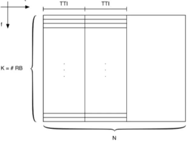
The usable resources are considered as a frequency-time period as depicted in Figure 3.1 with K RB for each TTI, which do not interfere each other. Instead of viewing the period as a matrix we can consider it like a vector of N ∗ K RB as depicted in Figure 3.2
Figure 3.2: Hyperframe Vector
3.2
Problem division
The problem, as explained in 3.1 , can be divided into three parts: Network Planning, Routing and Link Scheduling and Recovery. The three parts has different goals and periodicities.
The solutions adopted in the three parts do not affect each other and can be considered as three unrelated problems.The main components of the system are reported in Figure 3.3.
Figure 3.3: Problem Division
The system take in input a physical network deployment and returns a re-source allocation able to fulfill the network demands.
Network Planning phase analyze the physical deployment of the antenna in order to establish the architecture of the network. The result of this phase are: Connectivity Graph, specifying each connection among antennas, Conflict Graph that identify the interfering links and the Channel Quality Index (CQI) of each link representing the worst quality that a channel experiments.
Energy Efficient Routing and Link Scheduling given the traffic demands and the outputs of the previous section performs the resource allocation in order to fulfill each flows of the network. Routing and Link Scheduling algorithm aims to minimize the power consumed by the network and to maximize the reliability
of the paths.
Recovery permits to reroute demands in presence of a failure at a lower computation cost than recomputing the whole link schedule.
Each parts of the system will be analyzed in detail in Chapter 5, 6 ad in 7.
3.3
Software Implementation
In order to evaluate the proposed link-scheduler is needed to implement a simu-lator that, given a physical network deployment, carried out the system’s eval-uation. The simulator has been implemented using C + + language.
During implementation, particular attention was given to the reusability and the configurability of each part of the system.
In order to achieve this goal each block that composes the system (Figure 3.3) has been implemented as a stand-alone module.
This choice allowed us to create a library of reusable and configurable mod-ules to manage mesh networks.
The system is composed by the following modules : • Node deployment
• Network planning
• Energy efficient routing and link-scheduling • Recovery
4
Node Deployment
In this chapter we discuss about the Node deployment module. In section 4.1 we discuss the module’s objectives. The other parts of the chapter present the available type of deployment.
4.1
Target
The objective of this module is to provide a physical deployment of a network composed by two type of nodes: Macro and Micro nodes. In order to achieve this goal has been implemented a tool that permits to define the elements’ position. The elements can be deployed using one of the following criteria:
• Grid Deployment • Random Deployment • Configuration Deployment
4.2
Grid Deployment
The nodes are deployed in grid shape. The size of the grid and the distance between two adjacent nodes are configurable. In Table 4.1 is depicted a typical parameter configuration.
Parameter Name Distance (m) Configuration Number
dX 250 (i) dY 250 (ii) Min X 250 (iii) Max X 1250 (iv) Min Y 250 (v) Max Y 1250 (vi)
Table 4.1: Example of micro antenna configuration in grid deployment
Configurations (i,ii) impose horizontal and vertical distances, respectively, between two adjacent nodes. Configurations (iii,iv) and (v,vi) impose, respec-tively, the range of the horizontal and vertical deployments.
Given the parameter reported in Table 4.1 and in Table 4.2 the scenario deployed by the tool is shown in Figure 4.1.
4.3
Random Deployment
Nodes are deployed in a given area, the size of scenario and the number of each type of nodes are configurable as we can see in Table 4.3
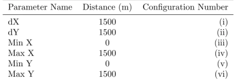
Parameter Name Distance (m) Configuration Number dX 1500 (i) dY 1500 (ii) Min X 0 (iii) Max X 1500 (iv) Min Y 0 (v) Max Y 1500 (vi)
Table 4.2: Example of macro antenna configuration in grid deployment
Figure 4.1: Grid Deployment
Configurations (i,ii) specifies the number of micro and macro nodes, the configurations (iii,iv) specifies the size of the scenario. Given the configuration specified in Table 4.3 the output of the tool is the deployment shown in Figure 4.2.
4.4
Configuration Deployment
Nodes deployment is specified using an input file. The input file specify in each line the parameters of the node to allocate. The configurable parameters are :
• Antenna Id • Position (x,y)
Parameter Name Distance (m) Configuration Number
Number of Micro 10 (i)
Number of Macro 3 (ii)
Max X 1000 (iv)
Max Y 1000 (vi)
Table 4.3: Example of parameter settings in random deployment
Figure 4.2: Random Deployment
• Gateway
An example of configuration file is reported in Listing 3. 0 1 100 100 1 0
1 2 500 100 1 0
2 3 500 500 1 1
3 4 100 500 1 0
4 5 600 600 1 0
5
Network Planning
In this chapter, we describe the network planning, this part of the system provide informations about connectivity and channel quality given a particular physical deployment.
In section 5.1 we discuss about the problem target. Sections 5.2 and 5.3 describe the graphs used during this phase. In section 5.4 the worst-caseCQI computing is carried out and explained as an optimization problem.
5.1
Problem Description
The objective of Network Planning is to determine which connections exist between the nodes and assign to each of them the worst-case CQI.
Given a node deployment the Network Planning phase returns in output : • Connectivity Graph
• Conflict Graph • Worst-Case CQI
The Connectivity Graph define which connection an antenna can establish, Conflict Graph specifying which communications can not be simultaneously and Worst-Case CQI define the channel quality in the worst-case.
5.2
Connectivity Graph
The network’s connections are modelled through the Connectivity Graph, G = (V, E) whose nodes V = {v1, ..., vn} are macro or micro nodes and whose edges
E = {e1, ..., em} are wireless links connecting a transmitter to a receiver.
The graph is computed evaluating the power received by a node and compar-ing it with the Connectivity Threshold. Given the antennas’ transmission power and the Connectivity Threshold we can define a transmission range for each antenna and so we can define every network’s connections. Figure 5.1 shows an example of the correspondence between physical deployment and Connectivity Graph. In green is depicted the antenna transmission range.
5.3
Conflict Graph
The Conflict Graph provide informations about which communications can not be simultaneous.
We have to take account to the physical interference phenomenon. For each edge of the network e ∈ E we define a conflicting set of edges I(e) which includes all the edges belonging to E which interfere with e.
The interference between two links implies a CQI reduction. We have to define a criterion to discriminate the conflicting link. One way to address the problem, and applied in this thesis, is to add the interference link into the conflict graph if the CQI, experienced by a node subjected to interference, is less than a certain CQIth.
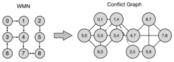
In the example shown in Figure 5.2 and in Table 5.1 the links : {1, 4; 0, 3; 2, 5} interfere with each other. In Table 5.1 are reported two cases of conflicting edges : {1,4; 0,3} and {1,4; 2,5}, the interferences are reported in the conflict graph with a dotted-line. The conflicts reported with a continuous line represents the protocol constraints3.
The use of CQIth is not the only way to discriminate the conflicting edge,
another way to account the problem is to define a maximum interference offset evaluating the interference caused by a link to the other. We translate the interference condition to a conflict graph Gc = (E, C) shown in Figure 5.2,
whose nodes are the set of links of the connectivity graph and whose edges C = (c1, ..., cr) model the conflicts within the network.
CQI
CQIth= 7 CQI threshold
CQI0(1,4)= 15 CQI on the link (1,4) without interference
CQI(2,5)(1,4)= 6 CQI on the link (1,4) with (2,5) interference
CQI(0,3)(1,4)= 5 CQI on the link (1,4) with (0,3) interference
CQI(5,8)(1,4)= 13 CQI on the link (1,4) with (5,8) interference
Table 5.1: Example of CQI interference
The criteria applied by the algorithm to compute the graph characterizing the network is explained in the next paragraphs.
5.4
Worst-Case CQI computing
The CQI on a certain transmission have to take into account the interference caused by the simultaneous transmissions done by other nodes of the network.
Figure 5.2: Logical connectivity graph (left) and conflict graph (right) of a WMN
The CQI computation have to be done for each edge of the connectivity graph. The Connectivity Graph labelled with the worst CQI value experimented by the edge its called Worst-Case Graph(Figure 5.3).
Figure 5.3: Worst Case Graph
Given a certain edge e its CQI value need to take account of the highest interference that edge e can experience, these CQI values its called Worst-case CQI cause are the minimum that the edges can experiments.
The maximum interference experimented by an edge is carried out by ap-plying a variation of the Stable Set Problem.
A stable set of a graph G is a set of nodes S with the property that the nodes of S are pairwise non adjacent. To achieve our purpose and calculate the maximum interference experimented by an edge we need to vary the stable set problem adding the interference on each node. The algorithm formulation is reported in section 5.4.1.
5.4.1 Problem Formulation
Given the Conflict Graph of the network CG = (V, E) and a certain edge k, of which we want to calculate the worst-case CQI, we define the problem as follows:
Maximize X i∈Vk xi∗ Pi,k Subject to xk= 1 (5.1) xi+ xj≤ 1 {i, j} ∈ CG (5.2) X e xe≤ 1 e ∈ OU T (v), ∀v ∈ V (5.3) X e xe≤ 1 e ∈ IN (v), ∀v ∈ V (5.4) xi∈ {0, 1}
OU T (v) = set of the edges outgoing from v IN (v) = set of the edges incoming in v
Pi,k= interference done by the edge i on the edge k
xi= equal to one if the edge is active
The objective function maximize the interference power experienced by the edge k. Constraint 5.1 impose to one the edge examined. This constraint impose that the edges adjacent to edge k are inactives. Constraint 5.2 impose that two adjacent nodes of the conflict graph cannot be active simultaneously. Constraints 5.3 and 5.4 avoid multiple transmission from or to an antenna. This model find the stable set of the conflict graph weighted with the interference power.
6
Routing and Link scheduling power efficient
algorithm
In this chapter, we propose a link scheduling algorithm, which take account of energy efficiency and reliability during the resource allocation process. In section 6.1 we define the problem and we introduce the targets. In section 6.2 we discuss the constraint in resource allocation and we define the algorithm as an optimization problem.
6.1
Problem description
The objectives of this phase are to provide routing and link scheduling that minimize the nodes’ power consumption, the delay experienced by a flow and maximize network’s reliability given the outputs of the network planning phase. Every link e has associated quantities such activation offset πe , 0 ≤ πe≤
(K ∗ N ) − 1, and transmission duration ∆e. Figure 6.1 shows the above
quan-tities.
Figure 6.1: Relevant quantities in link scheduling
A bit belonging to a flow experiences a delay dependent on the number of th ehop o fits path. Every hop in fact introduce a certain delay dependent on the amount of traffic managed by the nodes. We can estimate an upper bound dependent on the number of hop and the number of TTI, on which a schedule is composed, used by the algorithm (N ).
To better understanding the delay upper bound let’s consider the simple path of a flow shown in Figure 6.2. The flow goes from a source (s) to a destination (d) with three hops. The Worst Case Delay (WCD) experienced by this flow can be defined as follows:
W CD = numHop ∗ N
WCD of the path represented in Figure 6.2 with: numHop = 3
N = 3
Figure 6.2: Simple flow’s path
Figure 6.3: Worst-case delay
6.2
Formulation of the power efficient link scheduling
al-gorithm
Minimize (1−α)[X e Pe∗∆e+ X v,s onVv,s∗(Pbase,v−Pof f,v)]+α ∗ X e,q tqe∗ρq∗U NeSubject to : πi− πj+ ∆i ≤ (1 − oij) ∗ K ∀ i, j ∈ Cf (6.1) πj− πi+ ∆j ≤ oij∗ K ∀ i, j ∈ Cf (6.2) πi+ ∆i ≤ K ∗ N − 1 ∀ e ∈ E (6.3) X e∈OU T (v) tqe− X e∈IN (v) tqe= 1 if v = s(q) −1 if v = d(q) 0 otherwise ∀v ∈ V, ∀q ∈ Q (6.4) ∆e≥ X q∈Q ∆qe ∀ e ∈ E (6.5) ∆qe≤ K ∗ tq e ∀e ∈ E, ∀q ∈ Q (6.6) ∆q e N ∗ CQIe≥ ρq∗ t q e ∀ q if e ∈ Pq (6.7)
num hopPq∗ N ≤ Dmaxq ∀Pq (6.8)
num hopPq∗ N = X
e
tqe ∀e ∈ E, ∀q ∈ Q (6.9)
πe≥ onEe,s∗ s ∗ K ∀e ∈ E, ∀s (6.10)
πe+ ∆e≤ [(s + 1) ∗ K] + (1 − onEe,s) ∗ N ∗ K ∀e ∈ E, ∀s (6.11)
onVv,s≥ onEe,s
∀e ∈ IN (v) ∨ OU T (v)
∀v ∈ V (6.12)
X
s
onEe,s≥ tqe ∀e ∈ E, ∀q ∈ Q (6.13)
X
s
onEe,s≤ 1 ∀e ∈ E (6.14)
onEe,s≤ X q tqe ∀e ∈ E(6.15) oij ∈ {0, 1} 0 ≤ πi≤ (K ∗ N ) − 1 tqe∈ {0, 1} onVv,s∈ {0, 1} onEe,s∈ {0, 1} α ∈ [0, 1] xe, ye∈ N 0 ≤ s < N
∆e= number of resource blocks flowing through edge e
πe= activation offset of the edge e
ρq = rate of the flow q
U Ne= unreliability of the edge e
onEe,s= equal to one if the edge e is active during TTI s
onVv,s= equal to one if the node v is active during the TTI s
The objective function to be minimized take account of the power con-sumed by all the nodes of the network and aims to improve reliability. The first sum((1 − α)P
ePe∗ ∆e) takes into account the power consumed to
trans-mit the RBs on all the edges. The second sum (P
v,sonVv,s∗ (Pbase,v− Pof f,v))
consider the power consumption of a node to be turned on without transmitting.
The third sum (α ∗P
e,qt q
e∗ ρq∗ U Ne ) improve the reliability of the network
minimizing the rate of the unreliable flows. Alpha coefficient (α ∈ [0, 1]) de-termines which part of the objective functions assumes more importance in the minimizing operations. Keeping low traffic on the unreliable edge improves the reliability of the network. Constraints (6.1, 6.2) ensure that two conflicting flows do not overlaps as shown in Figure 6.4. Constraint (6.3) ensure that each link complete its transmission within the period duration. Constraint (6.4) ensure the flow conservation. In Figure 20 the node 1 is a source, node 2 is a desti-nation. Constraint (6.5) impose that the number of RBs allocated on a certain edge e is at least equal to the sum of the resource blocks allocated to the paths flowing through that edge. Constraint (6.6) impose an upper bound to the RBs allocated to a certain path flowing through an edge, the RBs transmitted can be at most K (3.1).
Figure 6.4: Overlapping Flows
Constraint (6.7) ensure that the rate of the RBs going through a certain edge e is at least the sum of the rate of the paths flowing through e. Constraint (6.8) impose an upper bound to the maximum delay experienced by a bit
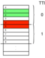
be-longing to a certain flow. Constraint (6.9) compute the number of hop of a path. Constraint (6.10, 6.11) does not allow resource assignments between adjacent TTI, Figure 7.5 shows two resource assignments : the green one is allowed, the red one is not permissible due to constraint (6.11). Constraints (6.12) ensure that when an edge, incoming or outgoing from a node v, is active the node v is active. Constraint (6.13) impose that if a flow goes through a certain edge e the edge is turned on at least in one TTI. Constraint (6.14) impose that an edge e is active at most for one TTI. Constraint (6.15) turn off the edge e if no flows going through that edge.
Figure 6.5: Flow Conservation
7
Recovery Problem
In this chapter, we describe the recovery phase, the third part of our problem as seen in Figure 3.3.
In section 7.1 a definition of the problem we want to solve is given. In section 7.2, we discuss the constraints in recovery problem and we describe the recovery problem as an optimization problem.
7.1
Problem Description
The problem we want to solve is to recover from a fail in the network in the shortest time possible.
The failure implies changes in the network topology and in the resource allocation made. The network’s section involved in the failure need to be re-scheduled and re-routed to ensure that all the flow are fulfilled. The re-routing have to take account of changes in the network due to node failure, the con-flict graph must be modified and the link-scheduling must take account about resources already reserved.
Suppose a network and its conflict graph shown in Figure 7.1, in case of failure of node 4 the conflict graph need to be modified as shown in Figure 7.2 where the links related to node 4 have been deleted. The re-routing decision need to take account of the new network topology and the new conflict graph. All the flow passing through the node 4 need to be re-routed and re-scheduled to find a new path going from source to destination.
Figure 7.1: Example Network
Figure 7.3 shows the path situation in case of node 4 failure. The left part of the figure shows the network and its path before the failure, the right part instead shows the network after the failure. Recovery phase involved only the flows that pass through the failed node, such flows reduction makes the recovery phase faster than the entire link-scheduling. The only flow that must be re-routed and re- scheduled, in this case, is the green one in dotted line. During
Figure 7.2: Example Network after the failure
the recovery phase only a subset of the original resources are allocable. Figure 7.4 shows the paths after the recovery phase, the green path has been re-routed through node 2 to reach its destination.
Figure 7.3: Network during node failure
Figure 7.4: Network’s path after recovery phase
As said before the usable resources in the recovery phase are limited. Sup-pose to have the network and its paths shown in Figure 7.3. The resource reservation, before the failure, is depicted in Figure 7.5 (a), when node 4 fail the resources allocated to flow 3 are no longer needed so they become free, as shown in Figure 7.5 (b). The recovery phase re-schedule flow 3 taking into account only the free resources (Figure 7.5 (b)).
Figure 7.5: Resource allocation before (a) and after (b) node failure
(Ed) become inactive. After the failure the flows can be divided into two subset : active flows, Fa ,and inactive flows, Fd. The flows become inactive , after the
failure, if in their path is present at least one inactive edge (Ed). The procedure
described above can be modelled as follows :
Vf = vi Va = {V − Vf} Ed= {e ∈ OU T (Vf) ∨ e ∈ IN (Vf)} Ea= {E − Ed} Fd= {∀q ∈ Q, ∀e ∈ Ed, e | e ∈ Pq} Fa= {Q − Fd}
The number of RB allocable in the recovery phase on a certain edge ( F reee
) can be calculated removing from all the resources assigned to an edge (K ∗ N ) the one allocated to the active flows after the failure (P
q∈Fa∆e,q∗ tqe) as follows : F reee= (K ∗ N ) − X q∈Fa ∆e,q∗ tqe
7.2
Problem Formulation
MinimizeX e Pe∗ X b Ze,b+ X v,s onVv,s∗ (Pbase,v− Pof f,v) + α ∗ X e,q tqe∗ ρq∗ U Ne Subject to : Zi,b+ Zj,b≤ 1 ∀ i, j ∈ Cf (7.1)onEe,s≥ Ze,b b ∈ (s ∩ F reee) (7.2)
X b Ze,b≥ X q∈Q ∆e, q (7.3)
onEe,s≥ onEe,s ∀e ∈ Ea, ∀s (7.4)
onVv,s≥ onVv,s ∀e ∈ Va, ∀s (7.5)
X e∈OU T (v) tqe− X e∈IN (v) tqe= 1 if v = s(q) −1 if v = d(q) 0 otherwise ∀v ∈ Va, ∀q ∈ Fa (7.6) ∆e= X q∈Q ∆e,q ∀e ∈ E (7.7) ∆qe≥ F reee∗ t q e ∀e ∈ E (7.8) ∆qe N ∗ CQIe≥ ρq∗ t q e ∀ q if e ∈ Pq (7.9)
onVv,s≥ onEe,s ∀e ∈ Ea, ∀e ∈ Va, ∀s (7.10)
X s onEe,s≥ t q e (7.11) X s onEe,s≤ 1 (7.12)
onEe,s− onEe,s≤
X q tqe (7.13) Vf ⊂ V Fd⊂ Q Fa⊂ Q 0 ≤ F reee≤ K ∗ N
Ze,b, onEe,s, onVv,s, tqe∈ {0, 1}
Vf = failed node
ed= inactive edge due to the failure Fd= set of flow to re-route and re-schedule Fa= set of active flow
Pq = path of the flow q
Q = set of all the flows
Ze,b = equal to one if the RB b is allocated for the edge e
onEe,s= equal to one if the edge e is active during the TTI s
onVv,s= equal to one if the node v is active during the TTI s
∆qe= number of RBs of the flow q going through edge e
tqe= equal to one if flow q going through edge e, zero otherwise
The objective function to be minimized take account of the power consumed by all the nodes of the network and aims to improve reliability. The first sum (P
ePe∗PbZe,b) consider the power consumed to transmit the RBs on all the
edges. The sum P
bZe,b represent the number of RB used by the edge e, as
depicted in Figure 7.6 the index e represent the edge number and the index b the RB number.
The second sum (P
v,sonVv,s∗ (Pbase,v− Pof f,v)) consider the power
con-sumed by a node when is turned on without transmitting. The third sum
(α ∗P
e,qt q
e∗ ρq∗ U Ne) aims to improve the reliability of the network
minimiz-ing the rate of the unreliable flows. Alpha coefficient (α ∈ [0, 1]) determines which part of the objective functions assumes more importance in the minimiz-ing operations.
Constraint 7.1 impose that two conflicting edges dont overlaps during trans-mission. Constraint 7.2 impose that an edge e is active during the TTIs if at least a RB of that edge is allocated. Constraints 7.3 impose that the number of RBs active on a certain edge e is at least equal to the number of RBs allocated to the paths going through the edge. Constraints 7.4 and 7.5 impose that an edge or a node, active before the failure, remains active after the failure. Con-straint 7.5 ensure the flow conservation. ConCon-straint 7.7 impose that the number of RBs allocated on a certain edge e is at least equal to the sum of the resource blocks allocated to the paths flowing through that edge. Constraint 7.8 impose an upper bound to the RBs allocated to a certain path flowing through an edge, the RBs transmitted can be at most F reee(Figure 7.5 ). Constraint 7.9 ensure
rate of the paths flowing through e. Constraints 7.10 ensure that when an edge, incoming or outgoing from a node v, is active the node v is active. Constraint 7.11 impose that if a flow goes through a certain edge e the edge is turned on at least in one TTI. Constraint 7.12 impose that an edge e is active at most for one TTI. Constraint 7.13 impose that if an edge e become active during routing and link scheduling at least one edge flows through that edge.
8
Performance evaluation
In this chapter, we evaluate the performance of the system described in the previous chapter.
In section 8.1, we describe the scenarios and the baseline used to evaluate the system’s performance. In section 8.2, using a tool network, is presented the network behaviour due to the change of input parameters. In section 8.3 and in section 8.4 the analysis and the results of the two analysed scenarios are reported.
8.1
Scenario
The scenarios that will be taken into account in this phase are the following: • Grid Deployment
• Ring Deployment
the scenarios’ analysis is carried out comparing the obtained result to the base-line (8.1.3).
8.1.1 Grid Scenario
The nodes are deployed in a grid shape. Micro deployment is carried out using the Grid Deployment tool (see 4.2).
8.1.2 Ring Scenario
The nodes are deployed in a ring shape. The deployment is provided using the Configuration Deployment tool (see 4.4)
The scenarios will be compared to the baseline presented in 8.1.3
8.1.3 Baseline
The baseline is an Heterogeneous Network (HetNet) composed by Macro and Micro node connected each other by a wireless one hop link. As explained in 2.3 the HetNet have been introduced in the past year to tackle the exponential growth of traffic demand and they’re employed in nowadays LTE deployment.
8.2
Preliminary Assumption
In this chapter a more detailed analysis is carried out to understand the system behaviour due to the input parameters’ changes.
Connectivity and Conflict threshold affects network topology and system behaviour. Connectivity Threshold affects the number of connection between
antennas, we expect that an increase of the Connectivity Threshold leads to a reduction of the edge number in the Connectivity Graph. The value of Conflict Threshold define which edge of the Connectivity graph goes into the Conflict Graph. A low Conflict Threshold value implies that more edge goes into the Conflict Graph, consequently simultaneous transmissions are more often avoided and the interference level is lower.
In order to show the network behaviour due to the thresholds’ change let us consider the node deployment example depicted in 8.1, the micro and macro settings are reported respectively in table 8.1 and in table 8.2.
Figure 8.1: Node Deployment Example
Node Type dX dY Min (X,Y) (m) Max(X,Y) (m) Tx Power (dBm)
Micro 100 100 100 300 8
Table 8.1: Micro Node Settings
Node Type X Y Tx Power (dBm)
Macro 100 100 10
Table 8.2: Macro Node Settings
The system’s behaviour due to Connectivity and Conflict Threshold change is depicted in Figure 8.2 and in Figure 8.3. Figure 8.2 shows how the edge
number is related to the Connectivity Threshold, Figure 8.3 shows the Conflict Threshold influence on the system. A higher Conflict Threshold implies fewer conflicts and more frequent simultaneous transmissions this causes a reduction of the average bit-rate of the network.
8.3
Grid Scenario
In this section the analysis of the grid scenario is carried out and the obtained results are presented.
In section 8.3.1, we introduce the baseline used to compare the results ob-tained. In section 8.3.2 a preliminary analysis of the grid scenario is carried out in order to tune the system’s parameter. In section 8.3.3 taking account to the preliminary assumptions we evaluate the scenario.
8.3.1 Baseline
Baseline’s parameters need to ensure the connectivity of the network, each link between Micros and Macro node need to be fulfilled, as shown in Figure 8.4. To ensure the above condition we need to analyse the system behaviour due to the power transmission change.
Figure 8.4: Grid Baseline : Connectivity Fulfilled
In Figure 8.5 is depicted the average bit-rate experimented by the network due to the Micros’ power transmission change.
The green line identify when all the uplink connections are fulfilled. The minimum value of macro’s transmission power to ensure downlink is lower than the value of the micro, we suppose that the value of the macro is at least equal to the micro. The analysis carried out on the baseline network implies the settings reported in Table 8.3.
Figure 8.5: Grid Baseline : Average Bit-Rate Trend
Node Transmission Power (dBm) Antenna Gain (dBm)
Micro 11 11
Macro 11 13
Table 8.3: Grid Baseline - Node Settings
8.3.2 Scenario Set-up
The considered scenario is depicted in Figure 8.6. The uplink transmissions represents the bottleneck of this scenario due to the lower micro transmission power. In order to achieve a full connected network at least one Micro need to be connected to the Macro (network’s gateway). The Micro transmission power in the case reported in Figure 8.6 must provide at least the connection between Micro 1 and Macro 0. The settings configuration that fulfil the above condition are reported in Table 8.4.
Configuration Micro Power (dBm) Connectivity Threshold (dBm)
A 9 -90
B 6 -93
C 3 -96
Table 8.4: Grid Scenario - Micro Node Settings
Figure 8.7 reports the analysis of the average bit-rate in the three proposed configurations, as we can see configuration “A” provide the best average bit-rate,
Figure 8.6: Grid Scenario
so it will be used in the analysis.
The settings of configuration “A” are the minimum necessary to ensure the connection from the Micro (1) to the Macro (0) but they result oversized for the other Micro involved in the scenario due to the antennas’ proximity. An oversized transmission power cause a greater number of conflicts between an-tennas . A high number of conflicts makes the transmissions more difficult. In order to avoid this situation we propose two level of Micro’s transmission power, the higher one (HighT P) will be used for the antennas closer to the Macro, the
lower (LowT P) will be used for the other ones.
The antennas further apart than a certain distance threshold from the macro will have a lower transmission power. Three threshold distances and two level of transmission power are defined as reported in Table 8.5 and 8.6.
Configuration Name Distance (m)
Step1 142
Step2 182
Step3 225
Table 8.5: Grid Scenario - Distance threshold
Configuration Name HighT P (dBm) LowT P (dBm)
PLH 9 8
PLL 9 6
Table 8.6: Grid Scenario - Power Level
In Figure 8.8 are reported the Micros involved in each configuration. In order to choose the best power transmission deployment it is necessary to analyse the system behaviour in case of PLH and PLL configurations.
The analysis of configurations PLH and PLL is carried out taking into ac-count the average bit-rate and the number of conflict between antennas.
As depicted in Figure 8.9, where the PLH configuration has been applied, the average bit-rate remains unchanged. The PLH power model application influence the number of conflict of the network. As shown in 8.10 the number of conflicts is less than in configuration “A”, this implies a greater number of simultaneous transmissions that increase the parallelism but they do not decrease the average bit-rate. As depicted in 8.11 the number of simultaneous transmissions is lower when configuration “A” is applied. The application of the PLH power level does not change the bit-rate and improves the network’s parallelism.
Figure 8.8: Grid Scenario - Step Configurations
Figure 8.9: Grid Scenario - Step Configurations Comparison : PLH
PLL configuration usage, in this case the average bit rate decreased compared to the configuration “A”. The observed decrease in average bit-rate makes the configuration unsuitable for our purpose.
The result of the preliminary analysis suggest to use the settings reported in Table 8.7.
Figure 8.10: Grid Scenario - Number of Conflict Comparison : PLH
Figure 8.11: Grid Scenario - Simultaneous Transmissions: PLH
Scenario Configuration Power Level Distance Threshold
Grid A PLH 142 (Step1)
Table 8.7: Grid Scenario - Settings
8.3.3 Scenario Evaluation
The metrics to be evaluated are the power consumed by the entire system and the traffic load that the system can handle. We evaluate the system’s behaviour