(will be inserted by the editor)
A perturbation approach for
the identification of uncertain
structures
Egidio Lofrano · Achille Paolone · Marcello Vasta
Received: date / Accepted: date
Abstract This paper deals with the identification of a linear structural systems with random parameters. The stiffness matrix of a four-storey shear frame structure is assumed to be linearly dependent by a random pa-rameter ruling the damage evolution of the columns. The evaluation of natural frequencies and the mode-shapes are in the context of random eigenvalue prob-lems in structural dynamics. A perturbation technique is first applied to derive the asymptotic solution up to the second order and to identify the mass and stiffness matrices. Then, the evaluation of the statistic of the frequencies and mode-shapes are derived up to the sec-ond order. Finally a stochastic identification technique is proposed to characterize the statistics of the random parameter.
Keywords Stochastic structural system identifica-tion· Uncertain structures · Perturbation approach
Egidio Lofrano
Department of Structural & Geotechnical Engineering, Sapienza University of Rome, Italy
18, Eudossiana St., 00184, Rome, Italy Tel.: +39-06-44585399
Fax: +39-06-488452
E-mail: [email protected] Achille Paolone
Department of Structural & Geotechnical Engineering, Sapienza University of Rome, Italy
Marcello Vasta
Engineering and Geology Department INGEO, University G. D’Annunzio of Chieti-Pescara, Italy
1 Introduction
The interest in the ability to monitor a structure and to detect its structural characteristics and damage at earliest possible stage is pervasive throughout the civil, mechanical and aerospace engineering communities. To this end, the number of identification techniques avail-able in literature have increased in the last twenty years [5]. These can be divided in two large group of tech-niques, namely the time domain identification techniques and the frequency domain identification techniques [6, 10]. A further classification of identification techniques consider the question when the input of the structure is unknown, undetectable or unmeasurable, called Output− Only identification techniques [3, 12] as these are based on response measurement only [14, 13].
In the safety assessment of many engineering struc-tures, randomness of various structural properties can be a crucial factor, especially when dynamic responses are of concern [4, 6, 2]. During structural dynamic analy-sis uncertainty is often present in structural parameters such as the material properties and dimensions. In the case of structural systems with random parameters one deals with stochastic structural system identification. However the probabilistic structure of these parame-ters is unknown in general and information need to be acquired via experimental setup. In literature many pa-pers deal with the direct problem, admitting a known form of the probabilistic structure of the parameters and then evaluating the response statistics (static or dynamic) of a given structure to an assumed distribu-tion of the parameters [11, 1]. However the inverse prob-lem for structure with uncertain parameter has received less attention and only few contributions are available in literature [8, 9]. There is a need therefore to develop ad hoc identification techniques taking into account the uncertain nature of the parameters and to identify their statistical properties. Although the uncertain nature of structure parameters seems reasonable and confirmed by experimental evidence, taking into account the sta-tistical nature of the parameters of a given structure increase the number of parameters to be identified as we will then be dealing with the statistics of these pa-rameters of any order. The natural way to achieve in-formation by experimental analysis is to proceed with the statistics of the acquired quantities. Under these circumstances it is necessary to incorporate probabilis-tic information into an overall model and to identify the statistics of the parameters, using both the model and available experimental data.
This papers focus on the estimation of the mean and variances of the parameters of a linear four-storey shear frame structure undergoing free vibrations. The
stiffness matrix is assumed to be linearly dependent by a random Gaussian parameter ruling the damage evolu-tion of the columns. The evaluaevolu-tion of natural frequen-cies and the mode-shapes are in the context of ran-dom eigenvalue problems in structural dynamics [1]. A perturbation technique [7] is first applied to derive the asymptotic solution up to the second order and to iden-tify the mass and stiffness matrices. Then, the evalua-tion of the statistic of the eigenvalues and mode-shapes are derived up to the second order. Finally an identifica-tion technique is proposed to characterize the statistics of the random parameter.
2 Direct problem: perturbative approximation of eigensolution statistics
Let be ε a Gaussian distributed random parameter with mean µεand variance σε2and M(ε), K(ε) the mass and stiffness matrices of a linear structure with no damping. The free vibrations of the structure are ruled by the following random matrix equation
M(ε)¨u(t) + K(ε)u(t) = 0 (1)
where u(t) represent the displacement vector of the structure. In modal analysis it is well known that the solution of the equation of motion are given by
u(t) =
n ∑ i=1
ϕiρisin(ωit + θi) = Φq(t) (2)
where n is the number of degree of freedom of the structure, q(t) the modal coordinate vector and Φ = [ϕ1· · · ϕn] the modal matrix. Inserting the displace-ment vector u(t) in Eq. (1) requires the solution of the following eigenvalue problem
{
(K(ε)− λiM(ε))ϕi = 0 λi= (2πfi)2
i = 1, . . . , n (3)
where λiand ϕi are the eigenvalues and eigenvectors of the dynamic system Eq. (1), and fi the corresponding frequencies.
Pointing out that the related random characteristic equation
det(K(ε)− λiM(ε)) = 0 i = 1, . . . , n (4) is nonlinear, in the following a perturbative approach will be considered [7]. For non defective systems, i.e., showing n distinct eigenvalues, it is possible to con-sider a Taylor expansion of the quantities of interest (fractional series expansions are needed for defective system).
Let us consider the Taylor series expansion of the mass and stiffness matrices around ε = 0
{ M(ε) = M0+ εM1+ ε2M2+ . . . K(ε) = K0+ εK1+ ε2K2+ . . . ∥ε∥ ≪ 1 (5) with Mj = 1 j! djM(ε) dεj ε=0 Kj= 1 j! djK(ε) dεj ε=0 (6)
The Taylor series expansion around ε = 0 can be con-sidered also for the eigenvalues and eigenvectors of the problem in Eqs. (3-4) { λi= λ0i+ ελ1i+ ε2λ2i+ . . . ϕi = ϕ0i+ εϕ1i+ ε2ϕ 2i+ . . . (7) with λji= 1 j! djλi(ε) dεj ε=0 ϕji= 1 j! djϕi(ε) dεj ε=0 (8)
Substituting Eqs. (5-7) in Eq. (3) and equating to zero the coefficients with the same power in ε, we obtain the following set of relationships
ε0: (K 0− λ0iM0)ϕ0i= 0 ε1: (K0− λ0iM0)ϕ1i= = (λ0iM1+ λ1iM0− K1)ϕ0i ε2: (K 0− λ0iM0)ϕ2i= = (λ0iM1+ λ1iM0− K1)ϕ1i+ +(λ0iM2+ λ1iM1+ λ2iM0− K2)ϕ0i . . . (9)
The perturbation procedure consider first the solution of the generating equation Eq. (9a), an eigenvalue prob-lem, to obtain the zero order solution (λ0i, ϕ0i). Then, one can solve Eq. (9b) to get (λ1i, ϕ1i), Eq. (9c) to get (λ2i, ϕ2i) and so on. It is worth noting that all these quantities are deterministic (as they do not depend on the random parameter ε) and that only one eigenvalue problem must be solved. It can be shown that the
per-turbative terms appearing in Eq.(9) are given by λ1i= ϕ⊤0i(K1− λ0iM1)ϕ0i ϕ⊤0iM0ϕ0i λ2i= ϕ⊤0i(K1− λ0iM1− λ1iM0)ϕ1i ϕ⊤0iM0ϕ0i + +ϕ ⊤ 0i(K2− λ0iM2− λ1iM1)ϕ0i ϕ⊤0iM0ϕ0i ϕ1i= αiiϕ0i+ n ∑ j=1 j̸=i ϕ⊤0j(K1− λ0iM1)ϕ0i (λ0i− λ0j)ϕ⊤0jM0ϕ0j ϕ0j ϕ2i= βiiϕ0i+ + n ∑ j=1 j̸=i (ϕ⊤ 0j(K1− λ0iM1− λ1iM0)ϕ1i (λ0i− λ0j)ϕ⊤0jM0ϕ0j + +ϕ ⊤ 0j(K2− λ0iM2− λ1iM1)ϕ0i (λ0i− λ0j)ϕ⊤0jM0ϕ0j ) ϕ0j (10)
where αii and βii are real coefficients that can be fixed imposing a normalization conditions.
Since in real life applications, the estimation of fre-quencies is more easy and reliable than the evaluation of mode-shapes, only the eigenvalue statistics are con-sidered in the following relationships. In detail, for the identification purpose, we start from Eq. (7a) and use the stochastic average operator E[•] in order to find the first and second order statistics of eigenvalues
E[λi] = λ0i+ E[ε]λ1i+ E[ε2]λ2i E[λiλj] = λ0i ( λ0j+ λ1jE[ε] + λ2jE[ε2] ) + +λ1i (
λ0jE[ε] + λ1jE[ε2] + λ2jE[ε3] )
+ +λ2i
(
λ0jE[ε2] + λ1jE[ε3] + λ2jE[ε4] )
(11)
Manipulating and simplifying Eqs. (11), the following relations for mean and covariance of λi are obtained µλi= λ0i+ µελ1i+ ( µ2 ε+ σ2ε ) λ2i+ o(ε2) σλiλj = σ 2 ελ1iλ1j+ 2σ2εµε(λ1iλ2j+ λ1jλ2i)+ +(2σ4 ε+ 4σε2µ2ε)λ2iλ2j+ o(ε2) (12)
obviously, if the λ2i, λ2j terms are neglected, a first or-der solution is employed; in this case, because of the lin-ear relationship between the eigensolution and the pa-rameter, also the eigenvalues appear as Gaussian vari-ables.
3 Inverse problem: identification of uncertain parameters
Different well posed techniques are available in litera-ture for the identification of the modal model of a struc-ture. They can be divided in time domain (e.g., Ibrahim Time Domain), frequency domain (e.g., Peak Picking)
and mixed time-frequency (e.g., Wavelet Based) identi-fication techniques. The main goal of these techniques consists in the identification of the main dynamic prop-erties of the structure, i.e. frequency and mode shapes [6].
In the framework of stochastic perturbation iden-tification techniques, the equations previously derived may be used to stochastically quantify the stiffness and mass matrix of a given structure. In particular, we as-sume that (M0, K0) are known matrices, obtained from the project analysis or from a preliminary experimental campaign; it is clear that in this work we are assuming these spatial quantities of the structure in its reference configuration as deterministic. Thus we proceed with the evaluation of the statistics of the uncertain param-eter from the knowledge of the measured and analytical eigenvalues statistics; since the random variables ε is as-sumed to be gaussian, its mean and standard deviation allow a complete statistical description of its PDF.
In our approach we also admit that the perturba-tive quantities (λ1i, λ2i, . . . ) are known, that is, we as-sume to known where the uncertain parameter acts; this assumption can be justified starting from the phys-ical meaning of the parameters. Since the formulation is designed for a dynamic system without damping, the range of possibilities is reduced to the analysis of alter-ations of mass or stiffness
– change in mass: it mainly occurs when one or more parts of the structure undergo a change of use or when a structural reinforcement is performed (in-deed, the variations for mass degradation and/or damage may be considered negligible);
– increase of stiffness: it occurs in the presence of a structural reinforcement;
– reduction of stiffness: it occurs when the structure is affected by a damage, visible or not.
In the first two cases, change in the mass and/or in-crease of the stiffness, the dependence of the model from the physical parameters representative of the structural changes can certainly be considered known a priori. For a stiffness reduction, i.e., a damage uncertain parame-ter, undoubtedly the most interesting case from an engi-neering point of view, in general the damage is not visi-ble (because the damage is not macroscopic or because the area is not accessible); in this case the dependence of the model from the parameter can be gathered em-ploying at upstream an ad hoc technique able to locate the damage, i.e., one of the so called level two damage identification technique [5].
Summarizing, in the applications under considera-tion the number of unknown is, regardless the perturba-tion order, equal to two, the couple (µε, σε); regarding
the number of equations, since in practical applications only a small number of eigenvalues can be measured, in what follows we will refer to an amount of measured eigenvalues nλ less than n and, accordingly, Eqs. (12) furnish 2nλgoverning relationships. As it is well known, a problem of this kind may be approached computing an objective function: to this aim we define the follow-ing functional E(µε, σε) = nλ ∑ i=1 ( 1− Kλ i Kλ˜ i )2 (13)
having indicated with K a fractile measure and where the amountKλiare analytic quantities, depending only by (µε, σε), while the termsKλ˜i represent the relevant measured counterparts. In other words, the objective function in Eq. (13) is a sum of squared errors defined as normalized eigenvalues discrepancies. Therefore, the proposed identification procedure belongs to the class of least square methods, for which the solving equation can be written in the form
(˜µε, ˜σε) = arg minE(µε, σε) σε≥ 0 (14) that is, we look for the couple (˜µε, ˜σε) that minimize the objective function with the constrain σε ≥ 0, plus relevant other constraints dictated by the physics of the problem (the mass and the stiffness of an element are strictly positive quantities).
The advantage of the proposed approach consists in the possibility of knowing the quantities (λ1i, λ2i, . . . ), that is to keep the advantages of the computational techniques based on perturbative approaches, regard-less of the chosen order of approximation. The following section discusses the choice of the fractile, while the sec-tion 4 shows an applicasec-tion of the proposed technique.
3.1 Choice of fractile
In the formulation of the objective function we pre-served the stochastic character of the problem express-ing the eigenvalues with reference to fractile measures. It’s a simple and intuitive method to account for un-certainties, and, moreover, it’s commonly used in the direct problem.
As regards the choice of the fractile, the calculation may not be so straightforward: even if the eigenvalue problem is a function of a Gaussian variable, usually the eigensolution is not (it is so only for first order so-lution). A simple solution to the issue, however, can be found through an alternative definition of fractile; if it’s regarded as an upper limit of the response [2], then we can simply put
Kλ
i = µλi+ 3 σλi (15)
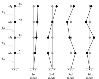
Fig. 1 Structural model and its unperturbed mode-shapes
(and similar for the measured quantities) where the choice of the value 3 comes from a similarity condi-tion with the value of the coefficient c such that if x is a Gaussian variable with mean µxand standard devia-tion σx, then
Kx = µ
x+ c σx (16)
has a probability of not exceeding equal to 99.9 %, ap-proximately.
4 Numerical example
Let us consider a four degrees of freedom planar struc-tural model as in Fig. 1, sketch on the left.
The equation of motion Eq.(1) can be written as follows (cfr. [4]) M1 0 0 0 0 M2 0 0 0 0 M3 0 0 0 0 M4 ¨ u1 ¨ u2 ¨ u3 ¨ u4 + + K1+K2 −K2 0 0 −K2 K2+K3 −K3 0 0 −K3 K3+K4−K4 0 0 −K4 K4 u1 u2 u3 u4 = 0 (17)
The following values of mass and stiffness are con-sidered Mi= 1 kg i = 1, 2, 3, 4 Ki= 1800 N/m i = 1, 2, 4 K3= 1800 (1− ε) N/m ε : p(ε) = N (µε, σε2) (18)
where p(ε) represents the probability density function (PDF) of the variable ε.
Table 1 Modal characteristics of the unperturbed system Mode λ0i, (rad/s)2 ω0i, rad/s f0i, Hz T0i, s
1 217.1 14.735 2.345 0.426 2 1800.0 42.426 6.752 0.148 3 4225.1 65.001 10.345 0.097 4 6357.8 79.736 12.690 0.079 DoF ϕ01 ϕ02 ϕ03 ϕ04 1 0.347 1.000 1.000 -0.653 2 0.653 1.000 -0.347 1.000 3 0.879 0.000 -0.879 -0.879 4 1.000 -1.000 0.653 0.347
Following the perturbative approach, Eqs.(6) return M0= 1 0 0 0 0 1 0 0 0 0 1 0 0 0 0 1 K0= 3600 −1800 0 0 −1800 3600 −1800 0 0 −1800 3600 −1800 0 0 −1800 1800 (19)
for the 0th-order terms,
M1= 0 K1= 0 0 0 0 0−1800 1800 0 0 1800 −1800 0 0 0 0 0 (20)
for the 1st-order terms,
M2= 0 K2= 0 (21)
for the 2nd-order terms.
For the unperturbed system (M0, K0), Table 1 shows the eigenvalues λ0i and the corresponding angular fre-quencies ω0i, cyclic frequencies f0i and periods T0i; in the same table are also listed the components of the eigenvectors ϕ0i, that are sketched in Fig. 1.
Two cases are taken under consideration – case 1 - deterministic: µθ∈ (0, 0.5], σθ2= 0;
– case 2 - stochastic : µθ∈ (0, 0.5], σ2θ= (0.05 µθ)2; that is, a deterministic/stochastic damage localized at the third level of the structure. The mean value is in-creased up to 0.5 in order to explore a wide neighbour-hood of the given configuration (50 % reduction of the third stiffness) and a constant coefficient of variation of the 5 % is considered to describe an increasing of dispersion with damage increasing.
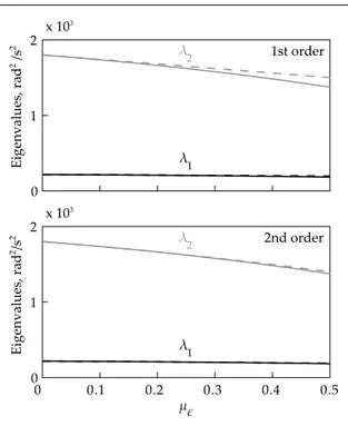
Fig. 2 Eigenvalues sensitivity, case 1
Hereafter we suppose that the first two frequencies has been detected during the tests (here numerically simulated). Before analyzing the inverse problem, in or-der to better interpret the results, we study the sensi-tivity of the eigensolution. The solution obtained with the perturbative approach (PA) using relationships (12) is compared with the solution of the eigenvalue prob-lem (1): for the deterministic case this can be easily done substituting the current value of µε (ES); for the stochastic case a Monte Carlo (MC) analysis was per-formed with up to 5000 simulations for each couple of (µε, σ2ε). The results are shown in Fig. 2, for case 1, and in Fig. 3, for case 2:
– caso 1 - deterministic: continuous line ES, dashed line PA;
– caso 2 - stochastic: continuous line MC, dashed line PA; thick and thin lines refer to mean and mean plus/minus three standard deviations values, respec-tively (although for the first eigenvalue λ1 the re-lated curves are practically indistinguishable). These figures show that, as suggested by the physics of the problem, the error committed by the perturbative approach increases by increasing the intensity of the sensitivity parameter ε, both in the deterministic (case 1) and stochastic (case 2) problem; it is also clear the contribution of the second order terms. To quantify the discrepancy when using the perturbative approach, the following comparisons are developed
– case 1 - deterministic: comparison between ES and PA;
Fig. 3 Eigenvalues sensitivity, case 2
– case 1 vs case 2: comparison among the mean val-ues obtained by the deterministic eigensolution (ES) and the ones obtained in the stochastic case by Monte Carlo simulations (MC);
– case 2 - stochastic: comparison between the mean values and the standard deviations given by Monte Carlo simultation (MC) with that obtained by the perturbative approach (PA).
The analysis of the numerical results allows for the following conclusions
– the continuous curves, for the case 1 (ES vs PA), and the dashed lines, for the case 2 (MC vs PA), of Fig. 4 show the percentage error in the mean val-ues evaluation. The error increase by increasing the mean value of the damage under consideration. The maximum error (in absolute value) is approximately equal to 10 and 4 %, for respectively first and second order approach;
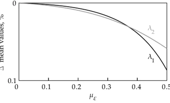
– the overlaps among the previous curves can be re-garded as a low influence of the parameter variance σ2
ε on the mean of the eigenvalues. This circum-stance is confirmed from an analytical point of view by the results in Fig. 5: the percentage discrepancy between the mean eigenvalues obtained by the de-terministic eigensolution (ES) and the ones obtained in the stochastic case by Monte Carlo simulations (MC) is less than 0.1 %;
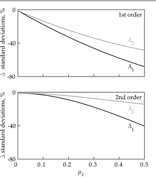
– in the stochastic case, the variations of the standard deviation (MC vs PA), Fig.s 6, highlight a maximum
Fig. 4 Percentage error for the mean values, cases 1 and 2
Fig. 5 Percentage error for the mean values, ES vs MC
error (in absolute value) of about 70 and 40 %, for respectively first and second order approach. These results suggest that, yet retaining the second or-der terms, the neighborhood properly identifiable in the inverse problem will shrink strongly going from the de-terministic to the stochastic case.
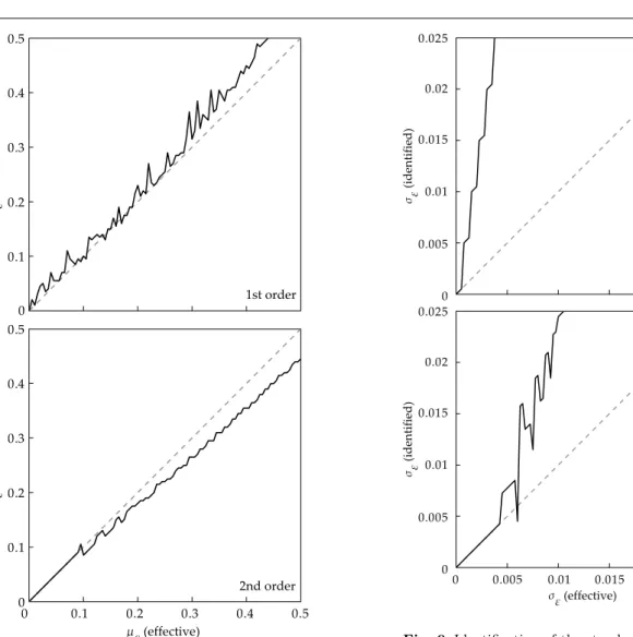
Going to the inverse problem, the experimental quan-titiesKλ˜i are here obtained numerically, starting from the solution of the eigenvalue problem (1): for the de-terministic case by replacing the value of the parameter µε, for the uncertain case performing a Monte Carlo simulation of 5000 samples drawn from a normal dis-tributionN (µε, σε2). Afterwards we try to identify the uncertain parameter applying the relationships (13-14). For the case 1, deterministic, the results obtained are those of Fig. 7, which contains both the the first and second order solutions for the identification of mean value of ε. Each of the graphs shows a dashed line, the bisector of the first quadrant of the effective-identified
Fig. 6 Percentage error for the standard deviations, case 2
plane of the parameter, representing the path of ideal minimum of the objective function (the identified pa-rameter equals the actual papa-rameter). In this manner, it’s easy to gather a qualitative measure of the goodness of the technique as the deviation of the obtained path, represented in the plots with a solid line, from the ideal (dashed) one. A similar convention is adopted for the case 2, stochastic, see Fig. 8, for the mean value, and Fig. 9, for the standard deviation.
Analyzing these results, it turns out that the error made in measuring the damage in our four degrees of freedom planar structural model can be void (in numer-ical limits) if
– deterministic damage: the stiffness reduction is smaller than 10 %, in the case of first order solution, and than 25 %, in the case of second order solution; – stochastic damage: the average stiffness reduction
is smaller than 10 % (corresponding to a standard deviation of 0.05 for the damage parameter, since a coefficient of variation of 5 % has been assumed) and at least a second order solution is adopted.
In other words, in the stochastic case not only the neigh-borhood properly identifiable is smaller than the one obtained for the deterministic case (as we expected from the sensitivity analysis), but also the second order terms become essential for a suitable implementation of the technique; indeed, if the first order solution suddenly tends to diverge from the effective statistics of parame-ter, the second order approximations is able to explore the neighborhood of the unperturbed solution.
Fig. 7 Identification of the mean value µε, case 1
5 Final remarks and further developments In this paper the identification of a linear structural sys-tems with random parameters is performed. The struc-tural system under consideration is a four-storey shear frame structure with a stiffness matrix linearly depen-dent by a random parameter ruling the damage evolu-tion of the columns. Using a perturbative approach the natural frequencies and mode-shapes are pursued in the context of random eigenvalue problems in structural dy-namics. The perturbation technique is first applied to derive the asymptotic solution up to the second order to identify the mass and stiffness matrices. Then, the evaluation of the statistic of the eigenvalues and mode-shapes are derived up to the second order. A stochastic identification technique is proposed to characterize the statistics of the quantities of interest and of the ran-dom parameter. Particular attention has been devoted in this paper with the identification of the first two frequencies of the structural system and to the mean
Fig. 8 Identification of the mean value µε, case 2
and variance of the random parameter assumed Gaus-sian without loss of generality. The numerical analy-sis show that the proposed identification technique is capable of identifying with very limited error the fre-quencies and the statistics of the random parameter. As further developments we mention here the question of non Gaussianity of the frequencies and mode-shape, the dependance of the parameters by a random vector (multiparametric case), the noise effect and finally the model updating and continuous model updating. All these aspects are under examination and will be tackle in the near future by the authors.
References
1. Adhikari, S., Friswell, M.I.: “Random eigen-value problems in structural dynamics”. 45th
AIAA/ASME/ASCE/AHS/ASC Structures, Struc-tural Dynamics & Materials Conference (2004)
Fig. 9 Identification of the standard deviation σε, case 2
2. Apley, D.W., Liu, J., Chen, W.: “Understanding the
ef-fects of model uncertainty in robust design with computer experiments”. Journal of Mechanical Design 128(1), 946–
958 (2006)
3. Brincker, R., Zhang, L., Andersen, P.: Modal
identifica-tion of output-only systems using frequency domain de-composition. Smart Materials and Structures 10(3), 441–
446 (2001)
4. Chopra, A.K.: “Dinamycs of structures”, Engineering
monographs on earthquake criteria, structural design, and strong motion records, vol. 2, 1a edn. Earthquake
engineering research institute (1980)
5. Doebling, S.W., Farrar, C.R., Prime, M.B., Shevitz, D.W.: “Damage identification and health monitoring of
structural and mechanical systems from changes in their vibration characteristics: a literature review”. Technical Report Los Alamos National Laboratory, LA-13070-MS
(1996)
6. Ewins, D.J.: “Modal testing: theory and practice”,
Engi-neering dynamics series, vol. 2, 1aedn. Research Studies
Press (1984)
7. Hajj, M.R., Fung, J., Nayfeh, A.H., Fahey, S.O.:
“Damp-ing identification us“Damp-ing perturbation techniques and higher-order spectra”. Nonlinear Dynamics 23(2), 189–
203 (2000)
8. Li, J., Roberts, J.B.: “Stochastic structural system
Compu-tational Mechanics 24(3), 206–210 (1999)
9. Li, J., Roberts, J.B.: “Stochastic structural system
iden-tification. Part 2: Variance parameter estimation”. Com-putational Mechanics 24(3), 211–215 (1999)
10. Maia, N.M.M., Silva, J.M.M.: “Theoretical and exper-imental modal analysis”, Engineering dynamics series, vol. 9, 1aedn. Research Studies Press (1997)
11. Manohar, C.S., Ibrahim, R.A.: “Progress in structural
dynamics with stochastic parameter variations: 1987 to 1996”. Applied Mechanics Reviews 52(5), 177–197
(1999)
12. Peeters, B., De Roeck, G.: “Stochastic System
Identifica-tion for OperaIdentifica-tional Modal Analysis: a review”. Journal of Dynamic Systems, Measurement, and Control 123(4),
659–667 (2001)
13. Roberts, J., Vasta, M.: “Markov modelling and
stochas-tic identification for nonlinear ship rolling in random waves”. Philosophical Transactions of the Royal Society of London. Series A: Mathematical, Physical and Engi-neering Sciences 358(1771), 1917–1941 (2000)
14. Roberts, J., Vasta, M.: “Parametric identification of
sys-tems with non-Gaussian excitation using measured re-sponse spectra”. Probabilistic Engineering Mechanics 15(1), 59–71 (2000)