An index of structural complexity for Apennine beech forests

Introduction

The theoretical and practical relevance of the structural attributes of forest stands is be-ing increasbe-ingly acknowledged (Franklin et al. 2002, Lindenmayer et al. 2000). Forest structure exerts a strong control upon biolo-gical diversity, since some structural compo-nents, such as coarse woody debris or cavity trees, provide resources and habitat for a wide range of species belonging to several taxonomic groups, such as birds, bats, in-sects, mosses, and lichens (Winter & Moller 2008, Brunialti et al. 2010, Jung et al. 2012). A broad interest exists in developing struc-ture-based indicators to use as proxies for other attributes that are difficult to assess. Several studies have tried to quantify the di-versity of forest structures in a stand through the definition of synthetic indexes. Some of these indexes were designed to rank forest stands on the basis of management intensity (Schall & Ammer 2013), developmental phases (Whitman & Hagan 2007) or

natural-ness (McRoberts et al. 2012), while others quantify the overall forest structural comple-xity, also referred to as structural heteroge-neity, based on several attributes (Staudham-mer & LeMay 2001, Zenner & Hibbs 2000, Houghton 2005).

Stand structural complexity is essentially a measure of the variety and relative abun-dance of different structural attributes in a given stand. Particular attention is usually paid to those attributes that quantify varia-tion (e.g., standard deviavaria-tion of tree diame-ters) because they directly describe habitat heterogeneity at the stand scale (McElhinny et al. 2005, Staudhammer & LeMay 2001). In forestry, structural heterogeneity is strictly related to the spatial pattern, size distribution and height variability of trees, whether living or dead. However, depending on the objec-tive of the study, other sources of complexity may be taken into account; for instance, vas-cular flora or litter distribution may still host certain organisms, modulate the resource

di-stribution and create patchy environmental conditions. Furthermore, structural comple-xity can be defined at different scales (e.g., plot, stand, forest or landscape scale), and each scale can be assumed to be important for specific categories of organisms, depen-ding on their size, dispersal ability and over-all “perception” of the physical environment. A stand-scale index of structural complexi-ty may facilitate the comparison of stands based on their potential contribution to bio-diversity (McElhinny et al. 2006, Whitman & Hagan 2007), since structural heterogene-ity is usually assumed to be correlated with different components of plant and animal di-versity (Neumann & Starlinger 2001, Bartels & Chen 2009, Brunialti et al. 2010, Taboada et al. 2010, Jung et al. 2012). Ideally, an index of structural complexity should be eas-ily applied by forest and land managers, and should use data routinely collected in Natio-nal Forest Inventories (NFIs) so as to be widely applicable (Chirici et al. 2011, Coro-na et al. 2011).

Ranking stands according to their struc-tural complexity may be challenging, since even ecologically similar forest stands within the same region may accumulate complexity in different ways (Donato et al. 2012). Struc-tural heterogeneity arises from the occur-rence of a number of different attributes whose complex interactions make its quan-tification an extremely difficult task (Whit-man & Hagan 2007). Furthermore, the rela-tive contribution of each structural attribute to forest complexity may vary consistently across systems. Indeed, different subsets of attributes have been used by different au-thors for calculating stand structural hetero-geneity in different regions and forest types, and all the proposed indexes are context-de-pendent to some extent (McElhinny et al. 2005).

(1) Department of Environmental Biology, University of Rome “La Sapienza”, p.le Aldo Moro 5, I-00185 Rome (Italy); (2) Dipartimento di Bioscienze e Territorio, Università degli Studi del Molise, c.da F.te Lappone snc, I-86090 Pesche (IS, Italy)

@

@

(francescomaria.sabatini@uniroma1.it) Received: Oct 22, 2013 - Accepted: May 21, 2014

Citation: Sabatini FM, Burrascano S, Lom-bardi F, Chirici G, Blasi C, 2015. An index of structural complexity for Apennine beech forests. iForest 8: 314-323 [online 2014-09-03] URL: http://www.sisef.it/iforest/ contents/?id=ifor1160-007

Communicated by: Renzo Motta

An index of structural complexity for

Apennine beech forests

Francesco Maria Sabatini

_{, Sabina Burrascano}

_{, Fabio Lombardi}

_,

Gherardo Chirici

_{, Carlo Blasi}

A broad interest exists in developing structure-based indicators to use as pro-xies for other attributes that are difficult to assess, such as biological diversity. Summary variables that account for stand-scale forest structural complexity could facilitate the comparison among stands and provide a means of ranking stands in terms of their potential contribution to biodiversity. We developed an index of structural heterogeneity (SHI) for beech forests in southern Italy: (i) we established a preliminary list of 23 structural variables obtained from data routinely collected in forest inventories; (ii) we quantified these variables in a set of 64 beech-dominated stands encompassing a wide range of variability in the Cilento, Vallo di Diano and Alburni National Park; (iii) we identified a core set of attributes that take into account the main sources of structural he-terogeneity identified in reference old-growth forests; and (iv) we combined these core attributes into a simple additive index (SHI). We identified eight core attributes that were rescaled to the range 0 to 10 using regression equa-tions based on raw attribute data. The SHI was calculated as the sum of these attribute scores and then expressed as a percentage. The index performance was evaluated against ten reference old-growth beech stands in the Apen-nines. The index ranged between 38 and 79.1 (median=59.4) and was distri-buted normally for the calibration dataset. The SHI successfully discriminated between old-growth (range=71.9-99.9, median=85.1) and early-mature to ma-ture forests. Furthermore, the SHI linearly increased with stand age and was higher in multi-layer high forests than in single- and double-layer forests. How-ever, a large variation was detected within both management types and age classes. SHI could be helpful for foresters as a tool for quantifying and compa-ring structural heterogeneity before and after a silvicultural intervention ai-med at restoring the structural complexity in second-growth stands.

Keywords: “Cilento, Vallo di Diano and Alburni” National Park, Fagus sylva-tica, National Forest Inventories, Old-growth Forests, Structural Heterogeneity Index

Recently, McElhinny et al. (2006) propo-sed an objective and quantitative methodo-logy for constructing an index of structural complexity that identifies key structures to take into account in a specific context. They first established a comprehensive suite of stand structural attributes. These attributes were then measured in a set of stands repre-senting the range of conditions occurring in a given region. From the analysis of these data, they finally identified a core set of at-tributes that were subsequently combined into a simple additive index, in which at-tributes were scored according to their over-all regional variability (McElhinny et al. 2006).

Here, we applied this methodology to de-velop a stand-scale index of structural he-terogeneity for Apennine beech forests. To identify the suite of attributes to include in this index of structural heterogeneity, we first explicitly defined the main sources of structural complexity commonly reported for beech natural forests in Italy and southern Europe. We considered old-growth condi-tion as the reference state, given that late successional forests, especially old-growth stands, are known to have a high horizontal

and vertical structural diversification (Piove-san et al. 2005, Bianchi et al. 2011, Calamini et al. 2011, Motta et al. 2011, Travaglini et al. 2012, Rugani et al. 2013, Sabatini et al. 2010, 2014).

The aim of our study was thus: (i) to de-velop an index of structural heterogeneity for southern Apennine beech forests; (ii) to test whether different age classes and forest ma-nagement types were characterized by diffe-rent levels of structural heterogeneity; (iii) to compare levels of structural heterogeneity among some well-studied reference old-growth beech stands in the Apennines and forest stands that do not display old-growth attributes.

We hypothesized that, with the exception of recently established stands, which were not considered in this work, stand structural heterogeneity increases with forest age, and differs according to the management type, with double- or multi-layered uneven-aged stands having significantly higher structural heterogeneity values than even-aged single-layered stands. We also expected old-growth to be more heterogeneous than other early-mature to early-mature forest stands.

Materials and Methods

Study area and data collection

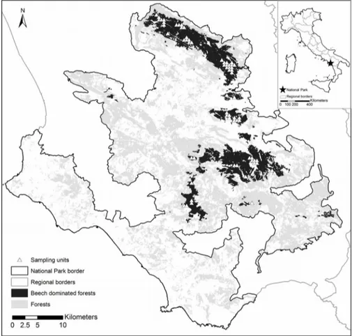
Data were collected in forest stands domi-nated by beech (Fagus sylvatica) in the Cilento, Vallo di Diano and Alburni Natio-nal Park (hereafter referred to as Cilento Na-tional Park), southern Italy (Fig. 1). We limi-ted our analysis to beech forests since they account for almost 10% of the Italian forests (more than 1 million ha, Gasparini & Tabac-chi 2011) and encompass 21.7% of the Cilento National Park. Furthermore, most of the remnant old-growth stands in southern Europe are dominated by beech. This has led to a body of knowledge being accumulated in recent years about the structure and varia-bility of this forest type under natural dyna-mics (Bianchi et al. 2011, Motta et al. 2011, Travaglini et al. 2012, Rugani et al. 2013, Sabatini et al. 2014).

Sampling units were identified based on an aligned systematic design, overlaying a 500 m grid on the beech forest distribution map. Plots were selected with the help of the Park planning records and photo-interpretation of digital aerial photographs (Flight IT2000, nominal resolution 1 m), with a nominal sca-le of 1:25.000. We excluded areas whose structural heterogeneity could derive from recent harvesting, i.e., by the creation of stumps and the co-occurrence of remnant trees (or standards) and very young trees. We focused on early-mature to mature fo-rests where structural heterogeneity is likely due to natural forest dynamics (tree senes-cence and death, establishment of natural re-generation and gap dynamics, etc).

Overall, 64 sampling units across 12 forest areas were selected, encompassing an area of about 137 km2 _{(Fig. 1). These included}

stands diversely managed, ranging from cop-pices with different standard densities, to even- and uneven-aged high forests. Some of the stands showed old-growth features, such as large old trees, logs and snags.

A circular plot of 20-m radius (1256 m2₎

was established in each unit. Living trees in each plot were calipered in concentric circu-lar areas with a radius of 4, 13 and 20 m, with thresholds of minimum diameter at breast height (DBH) of 2.5, 10 and 50 cm, respectively. Height was measured using a Haglof Vertex on one out of ten sampled trees, chosen randomly. For the remaining trees, the height was estimated with a tradi-tional H=f(DBH) model calculated on the basis of the trees whose height was mea-sured. In the intermediate circular area (13 m radius), the length and diameter of all the ly-ing deadwood components (with a minimum diameter ≥ 10 cm) were measured, as well as their decay level according to Hunter (1990). The age of each stand was estimated in the field by expert opinion on the basis of evi-dence of past disturbance or harvest, as well

Fig. 1 - Distribution of forests in the Cilento, Vallo di Diano and Alburni National Park.

Forests (light gray), beech forests (dark gray) and location of the sampling units within the beech forests (white triangles) are shown.

as on the mean size of canopy trees. Age was assigned to one out of six broad classes (1: < 50 yrs; 2: 50-80; 3: 80-100; 4: 100-120; 5: 120-140; and 6: > 140 yrs old). Stands were classified according to their management type and structure in the following groups: single-, double-, and multi-layer high forests, and coppices. The distribution of estimated ages across forest types is reported in Fig. S4 (Appendix 4). For a more detailed descrip-tion of the forest structure data collecdescrip-tion and preliminary analysis, see Blasi et al. (2010) and Burrascano et al. (2011).

As an additional dataset, we selected 10 beech-dominated stands in central Italy with old-growth features (such as high density of large living trees, high amount of deadwood, uneven-aged structure), whose high struc-tural heterogeneity was previously reported in several studies (Piovesan et al. 2005, Bur-rascano et al. 2008, Lombardi et al. 2010, Sabatini et al. 2010, 2014, Calamini et al. 2011, Travaglini et al. 2012). Information on location, climate, underlying bedrock and time since last disturbance of these stands is provided in Tab. S1 and Fig. S1.1 (Appen-dix 1).

Living trees and deadwood were sampled within a 1 ha plot in all the study sites except two (Cozzo Ferriero, 0.16 ha; Fosso Cecita, 0.45 ha), in which plot size was reduced be-cause of the very steep slopes. The position, species, DBH (minimum threshold of 3 cm) and height of every tree in the plot were recorded, as well as the position, diameter and length (or height) of standing dead trees, downed dead trees, snags and stumps. Dead-wood pieces were sampled if they met the following requirements: minimum diameter > 5 cm, more than half the base of their thicker end lying within the plot, length > 1 m. Further details are reported by Lombardi et al. (2010) and Calamini et al. (2011).

Selection of structural variables to be

included in the Index

An index of structural heterogeneity was built according to the methodology proposed by McElhinny et al. (2006). This four-stage approach starts from (i) the definition of a comprehensive suite of structural attributes that are (ii) then sampled and analyzed in or-der to (iii) identify a core set of attributes and (iv) combine them into an index.

We compiled a preliminary list of 23 struc-tural variables that may easily be derived from routinely collected data in forest moni-toring programmes and NFIs (Chirici et al. 2011). This list comprised: (1) basal area; (2) growing stock; (3) number of DBH classes; (4) DBH diversity (calculated using the Gini-Simpson Index); (5) DBH range; (6) number of living trees with DBH>40cm; (7) tree species richness; (8) quadratic mean DBH; (9) living stem density; (10) height; (11) height standard deviation; (12) snags

volume; (13) standing dead trees volume; (14) Total standing deadwood volume; (15) density of standing deadwood (both snags and standing dead trees); (16) basal area of standing deadwood (both snags and standing dead trees); (17) stumps volume; (18) lying coarse woody debris volume; (19) the loga-rithm of the sum of the lengths of lying coarse woody debris pieces (hereafter re-ferred to as “total log length”); (20) total deadwood volume; (21) ratio between dead-wood and living dead-wood volumes; (22) num-ber of decay classes occurring in the plot; (23) coarse woody debris index (CWDI, see Appendix 2 for calculation according to Mc-Elhinny et al. 2006).

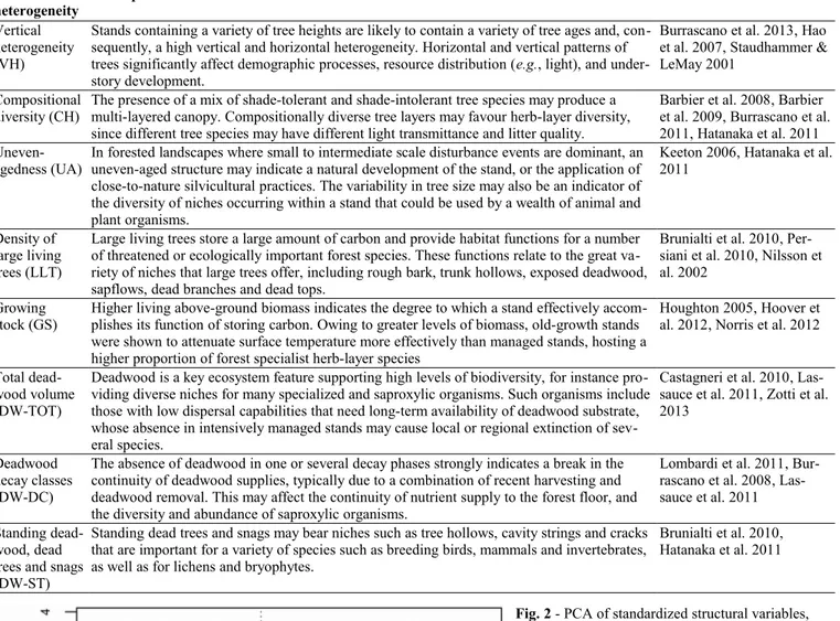
To define the suite of attributes to be con-sidered in the final core set of attributes, we first listed the main sources of structural complexity occurring in beech natural fo-rests, as reported in recent literature on old-growth forests in southern Europe (Piovesan et al. 2005, Bianchi et al. 2011, Calamini et al. 2011, Motta et al. 2011, Travaglini et al. 2012, Lombardi et al. 2012, Rugani et al. 2013, Sabatini et al. 2014). We considered above all sources of heterogeneity correla-ting with other desirable properties, e.g., plant and fungi biodiversity, faunal habitat availability and carbon stocking (Houghton 2005, Burrascano et al. 2008, Blasi et al. 2010, Taboada et al. 2010, Hatanaka et al. 2011, Zotti et al. 2013). Eight sources of structural complexity were considered: (1) vertical heterogeneity; (2) compositional di-versity; (3) uneven-agedness; (4) density of large living trees; (5) growing stock; (6) total deadwood volume; (7) deadwood decay clas-ses; (8) standing dead trees and snags. A brief description of these elements and how they relate to other ecosystem properties are reported in Tab. 1.

When designing an index of structural complexity, one should focus on attributes that: (i) have a low kurtosis, since a high kurtosis would indicate similar values of an attribute for several sites; (ii) may help to distinguish between categories of interest (e.g., early- versus late-successional stands); (iii) are proxies of other variables or origi-nally contribute to the overall structural stand complexity; (iv) are easily measurable in the field (McElhinny et al. 2006, Chirici et al. 2011).

Both logarithm and square-root transfor-mations were applied to improve the distri-bution of attributes showing a high kurtosis (<2): in the selection stage, we only retained the transformation that most improved their distribution.

Since we assumed that structural comple-xity increases with age, early- and late-suc-cessional stands were separated choosing an age threshold of 100 years (which represents the usual harvest return interval for beech forests in the Apennines) and then

com-pared. Differences between the two men-tioned groups were tested for each structural variable by Mann-Whitney test.

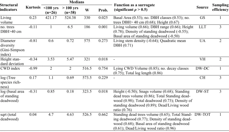
Pairwise correlation between variables was calculated using the Spearman’s ρ coeffi-cient. To visualize the multi-correlation structure of variables and evaluate their re-dundancy, we performed a Principal Compo-nents Analysis (PCA) and represented it in Gabriel’s plots (only the first 2 principal components, accounting for 42.3% of the to-tal variance, are shown in Fig. 2).

To help in variable selection, we also esti-mated whether they were more or less diffi-cult to sample and/or calculate. Variables that only need tree diameter data (e.g., Gini-Simpson’s diversity, basal area) were consi-dered having a sampling efficiency higher than variables requiring the estimation of other parameters, such as tree height or deadwood debris decay class. To this purpo-se, variables were grouped in 3 sampling ef-ficiency classes (1: low to 3: high). When se-lecting between two or more highly corre-lated variables to be included in the index, those with a high sampling efficiency were favored (see Appendix 3).

Finally, we created a core set of structural attributes that included a variable for each of the eight sources of structural complexity listed in Tab. 1. Considering the first source of structural complexity (VH), the variable best describing this feature (height standard deviation) was included, provided that it matched the four selection criteria listed above. A similar procedure was adopted for the next sources of structural complexity un-til all eight sources were represented in the core set. We took tha additional care that the new variable added to the set had the lowest correlation with the variables included in the previous steps. If no variable matched all the selection criteria for a given source of com-plexity, variables showing low kurtosis and low correlation with those already included were favored. The eight structural variables included in the core set are listed in Tab. 2.

Construction of a Structural

Heterogeneity Index (SHI)

A score ranging from 0 to 10 was assigned to each attribute in the core set based on li-near regression through quartiles (Tab. 3). We first set a score of 2.5, 5, 7.5 and 10 to the quartile midpoints (corresponding to the 12.5, 37.5, 62.5 and 87.5 percentiles, respec-tively) of the raw attribute distribution. Then, a linear regression through quartile values was fitted to ensure that the attribute scores were evenly distributed between 0 and 10. This regression equation was used to associate a score with each observation. Re-gression was constrained between 0 and 10 to prevent extremely low and high values from taking scores outside the range. The maximum attribute score of 10 was

attri-Fig. 2 - PCA of standardized structural variables,

axes 1-2. (Green): Live trees structural variables; (Red): Deadwood-related variables; (Blue): Tree Height-related variables. (BA): Basal area; (RangeDBH): range of diameter distribution; (QMDBH): quadratic mean diameter; (LivVol): growing stock; (Ndbh): number of diameter classes; (StemDens): Stem density; (TreeRich): tree species richness. (CWD): Coarse woody debris volume; (Stumps): volume of stumps; (Snags): volume of standing dead trees broken above 1.3 m; (StDw): volume of standing dead trees; (SnagStDw): volume of standing dead trees (including snags);

(NsnagsStDW): number of standing dead trees (in-cluding snags); (BASnagSt): basal area of standing dead trees (including snags); (DWtot): Deadwood (standing + CWD) total volume; (DWLivRatio): li-ving wood/Deadwood volume ratio; (CWDI): coarse woody debris index (see Appendix 2);

(DwlogLength): log of the sum of lengths of every coarse woody debris piece; (H): mean height; (Hsd): height standard deviation.

Tab. 1 List of the eight sources of structural heterogeneity considered in the present study and their ecological importance for forest biodi

-versity. This list represents the basis to select the structural attributes for constructing the SHI (Structural Heterogeneity Index).

Sources of structural

heterogeneity Description References

Vertical heterogeneity (VH)

Stands containing a variety of tree heights are likely to contain a variety of tree ages and, con-sequently, a high vertical and horizontal heterogeneity. Horizontal and vertical patterns of trees significantly affect demographic processes, resource distribution (e.g., light), and under-story development.

Burrascano et al. 2013, Hao et al. 2007, Staudhammer & LeMay 2001

Compositional

diversity (CH) The presence of a mix of shade-tolerant and shade-intolerant tree species may produce a multi-layered canopy. Compositionally diverse tree layers may favour herb-layer diversity, since different tree species may have different light transmittance and litter quality.

Barbier et al. 2008, Barbier et al. 2009, Burrascano et al. 2011, Hatanaka et al. 2011

Uneven-agedness (UA) In forested landscapes where small to intermediate scale disturbance events are dominant, an uneven-aged structure may indicate a natural development of the stand, or the application of close-to-nature silvicultural practices. The variability in tree size may also be an indicator of the diversity of niches occurring within a stand that could be used by a wealth of animal and plant organisms.

Keeton 2006, Hatanaka et al. 2011

Density of large living trees (LLT)

Large living trees store a large amount of carbon and provide habitat functions for a number of threatened or ecologically important forest species. These functions relate to the great va-riety of niches that large trees offer, including rough bark, trunk hollows, exposed deadwood, sapflows, dead branches and dead tops.

Brunialti et al. 2010, Per-siani et al. 2010, Nilsson et al. 2002

Growing

stock (GS) Higher living above-ground biomass indicates the degree to which a stand effectively accom-plishes its function of storing carbon. Owing to greater levels of biomass, old-growth stands were shown to attenuate surface temperature more effectively than managed stands, hosting a higher proportion of forest specialist herb-layer species

Houghton 2005, Hoover et al. 2012, Norris et al. 2012 Total

dead-wood volume (DW-TOT)

Deadwood is a key ecosystem feature supporting high levels of biodiversity, for instance pro-viding diverse niches for many specialized and saproxylic organisms. Such organisms include those with low dispersal capabilities that need long-term availability of deadwood substrate, whose absence in intensively managed stands may cause local or regional extinction of sev-eral species.

Castagneri et al. 2010, Las-sauce et al. 2011, Zotti et al. 2013

Deadwood decay classes (DW-DC)

The absence of deadwood in one or several decay phases strongly indicates a break in the continuity of deadwood supplies, typically due to a combination of recent harvesting and deadwood removal. This may affect the continuity of nutrient supply to the forest floor, and the diversity and abundance of saproxylic organisms.

Lombardi et al. 2011, Bur-rascano et al. 2008, Las-sauce et al. 2011 Standing

dead-wood, dead trees and snags (DW-ST)

Standing dead trees and snags may bear niches such as tree hollows, cavity strings and cracks that are important for a variety of species such as breeding birds, mammals and invertebrates, as well as for lichens and bryophytes.

Brunialti et al. 2010, Hatanaka et al. 2011

buted to the 87.5 percentile. Compared with a simple scaling of values in the range -1 to 1, the above technique has the advantage of avoiding possible distortions due to the oc-currence of extremely high or low outliers, and yielding a more even distribution of in-dex scores across the range of variability of the raw attributes.

Finally, a Structural Heterogeneity Index (SHI) was obtained by summing the scores in the range 0-10 assigned to each variable in the core set, and then expressed as a per-centage. Score weighting was not considered here because: (i) it could imply an arbitrary choice; (ii) index performances were found to be independent of the weighting of at-tributes (McElhinny et al. 2006); (iii) an un-weighted index provides a clearer picture of the relative contribution of different sources of heterogeneity.

Testing the Structural Heterogeneity

Index

SHI values calculated for the 64 forest plots in the Cilento National Park were tested for significant differences between broad classes based on age and management type using non-parametric Kruskal-Wallis test. We used multiple regression to test whether the SHI significantly increases with

age, and covariates with management type as well as with other environmental attributes (i.e., altitude, slope, aspect). Backwards se-lection was applied to discard non-signifi-cant terms.

As an additional evaluation of index per-formances, we calculated the SHI on the set of 10 beech-dominated, old-growth forests from central Italy (Fig. S1.1, Tab. S1 - Ap-pendix 1), whose structural data were not used during the calibration process. SHI va-lues of such forests were compared with those obtained for plots in early-mature to mature stands in the Cilento National Park. We tested for significant differences by

means of the Kruskal-Wallis test.

All analyses were performed using the soft-ware package R 2.14.1 (R Development Co-re Team 2011).

Results

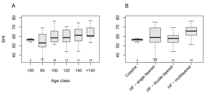
Beech stands in the Cilento National Park showed index values ranging between 38 and 79.1 (median 59.4) and showing no de-parture from normal distribution (Fig. S5.1). The SHI appeared to have a minimum in the 80 year-age class, and a slow increase with age (Fig. 3A). A high variability of SHI va-lues was observed within each age class, and no significant differences among classes

Tab. 2 Core set of structural variables and selection criteria. (W): Wilcoxon test (equivalent to MannWhitney); (Source): the source of he

-terogeneity indicates whether the variable could be a proxy of one of the eight features described in Tab. 1; (VH): vertical he-terogeneity; (CH): composition heterogeneity; (UA): uneven-agedness; (LLT): occurrence of large living trees; (GS): high growing stock; (DW-TOT): occurrence of a relatively high deadwood volume; (DW-DC): occurrence of deadwood in different decay classes; (DW-ST): occurrence of standing deadwood, dead trees and snags. Sampling efficiency: 1 - poor, 2 - medium, 3 - high.

Structural

indicators Kurtosis

Medians

Function as a surrogate

(significant ρ > 0.5) Source Samplingefficiency

<100 yrs

(n=26) > 100 yrs(n=38) W Prob.

Living volume

0.23 421.17 524.38 330 0.025 Basal Area (0.53); no. DBH classes (0.53); no. trees DBH> 40 cm (0.68); Height (0.67)

GS 1

no. trees

DBH>40 cm -0.11 1 6.5 186 0.001 Living volume (0.66); DBH range (0.66); Height(0.78); Density of standing deadwood (-0.55); Basal area of standing deadwood (-0.50)

LLT 3

Diameter diversity (Gini-Simpson index)

-0.81 0.6 0.72 575 0.273 Living stem density (-0.64); Quadratic mean

DBH (0.71) UA 2

Height stan-dard deviation

-0.34 3.53 5.47 321 0.018 - VH 2

CWD index -0.99 2 2 516.5 0.754 Lying CWD Volume (0.85); no. decay classes

(0.75); Total log length (0.86) DW-DC 1

log (Tree species rich-ness)

0.17 1.1 0.69 573.5 0.229 - CH 3

log (basal area of standing deadwood)

-0.31 0.85 0.18 323.5 0.018 Height (-0.50); Snags volume (0.68); Standing dead trees volume (0.86); Total Standing dead-wood (0.98); Total deaddead-wood (0.73); Density of standing deadwood (0.89); Dead/Living wood ratio (0.76)

DW-ST 3

sqrt (total deadwood)

0.04 4.7 4.63 526.5 0.662 Standing dead trees volume (0.65); Total Stand-ing deadwood (0.77); Density of standStand-ing dead-wood (0.68); Basal area of standing deaddead-wood (0.61); Dead/Living wood ratio (0.96)

DW-TOT 1

Tab. 3 - Regression equations used to assign a score to attributes on a scale of 0-10,

ob-tained from 64 beech dominated forest stands in the Cilento, Vallo di Diano e Alburni Na-tional Park, southern Italy. For more details, see Materials and Methods.

Attribute Regression equation R2

Living volume Score = -2.021 + X · 0.016 0.938

no. Large Living Trees DBH> 40 cm Score = 3.274 + X · 0.595 0.952 DBH diversity (Gini-Simpson index) Score = -2.233 + X · 14.034 0.969 Height standard deviation Score = 1.815 + X · 0.811 0.918

CWD index Score = 3.750 + X · 1.25 0.900

Log (Tree species richness) Score = -2.511 + log(X) · 9.053 0.900 Log (basal area of standing deadwood) Score = 3.536 + log(X) · 4.221 0.924 sqrt (Total deadwood volume) Score = 1.167 + sqrt(X) · 1.083 0.999

(Kruskal-Wallis H = 6.08, df = 5, p = 0.297). On the other hand, the SHI significantly dif-fered across management types (H = 10.39, df = 3, p = 0.015). However, the only signifi-cant (p<0.05) difference using post-hoc

tiple comparison was detected between mul-ti-layer and double-layer high forests (Fig. 3B). Multiple regression showed a signifi-cant linear increase in the SHI with stand age (b = 0.064, t(61) = 2.48, p = 0.015) and a

ne-gative relationship with altitude (b = -0.022, t(61) = -3.31, p = 0.002). Adjusted-R2 was

0.19. Based on the above analysis, neither management type, nor the interaction be-tween management type and age, were sig-nificant predictors of the SHI.

Structural heterogeneity of a set of

Italian beech old-growth forests

The SHI of the selected old-growth stands ranged between 71.7 and 99.9 (median 85.1). The SHI was significantly higher for reference old-growth stands than for the beech stands included in the main dataset (H = 27.7, df = 2, p < 0.001 - Fig. 4, Tab. 4).

The high SHI values observed in the old-growth stands stem from the high scores of index subcomponents, whose relative impor-tance varied greatly across stands (Tab. 4). According to the SHI, each of the 10 old-growth stands was structurally heteroge-neous in a unique way; the most important sources of SHI variability among old-growth stands were living volume, tree height

stan-Fig. 3 - Boxplot of SHI across age classes (A) and structural types (B). Small numbers below the boxes represent the sample size. (HF): High

forest.

Fig. 4 - SHI comparison

be-tween early-mature to ma-ture, and old-growth stands. The boxplots refer to the SHI of managed beech forests in the Cilento Na-tional Park (left) with those of a set of beech forests with old-growth features located throughout the Apennines (right). Small numbers be-low the boxes represent the sample size.

Tab. 4 SHI values and scores for its subcomponents calculated for 10 beech stands with oldgrowth features located throughout the Apen

-nines. Scores for each structural variable was obtined by the regression equations reported in Tab. 3. SHI was calculated as the sum of va-riable scores, normalized on a percent basis.

Stand _volumeLiving _{DBH>40 cm}No. trees _{(Gini-Simpson)}DBH diversity Height_sd CWD_index (tree sp.Log richness) Log (BA stand dw) Sqrt (total dw) SHI Abeti Soprani 6.9 10.0 10.0 6.8 10.0 10.0 9.4 10.0 91.4 Collemeluccio 6.7 10.0 10.0 6.6 10.0 10.0 4.8 5.7 79.8 Cozzo Ferriero 10.0 10.0 10.0 8.4 10.0 0.0 7.1 10.0 81.8 Fonte Novello 10.0 10.0 10.0 7.3 10.0 0.0 10.0 10.0 84.1 Gargano-Pavari 8.4 10.0 10.0 10.0 10.0 7.4 9.1 10.0 93.7 Monte Cimino 10.0 10.0 9.3 10.0 10.0 10.0 5.0 7.3 89.5 Monte di Mezzo 9.0 10.0 10.0 7.8 10.0 10.0 5.4 6.7 86.2 Monte Sacro 5.3 10.0 8.3 7.9 10.0 0.0 5.9 10.0 71.7 Sasso Fratino 10.0 10.0 10.0 10.0 10.0 10.0 10.0 9.9 99.9 Val Cervara 3.7 10.0 8.6 8.6 10.0 0.0 10.0 10.0 76.1

dard deviation, canopy tree species richness and basal area of standing deadwood. For in-stance, living volume greatly varied across the 10 old-growth stands, probably as a re-sult of differences in altitude, site fertility and time since last disturbance. Although “Val Cervara” is probably the best preserved old-growth beech stands in central Apenni-nes, this stand only attained a very low score for living volume (3.7 out of 10), when com-pared with other stands located at lower alti-tudes and in more favorable site conditions (e.g., “Fonte Novello” or “Monte Cimino”). The basal area of standing deadwood also strongly varied across stands (from 4.8 in “Collemeluccio” to 10 in “Fonte Novello”, “Sasso Fratino” and “Val Cervara”). Species richness of the tree layer varied markedly and clearly distinguished between pure beech stands (e.g., “Fonte Novello”, “Val Cervara”) and beech stands mixed with other taxa such as Abies alba (e.g., “Abeti So-prani”, “Sasso Fratino”), or other broad-leaved species, such as Ilex aquifolium and Acer obtusatum in “Gargano-Pavari”, or A. obtusatum and A. pseudoplatanus in “Monte Cimino”.

Discussion

Management, disturbance history, and

environmental factors contribute to

current forest heterogeneity

We applied an acknowledged methodology to obtain an index of structural heterogeneity for southern Italy beech forests. Forest struc-tural heterogeneity, as indicated by the SHI, linearly increased with stand age and was higher for multi-layer high forests than for single- and double-layer forests.

The positive relationship between the SHI and stand age closely matched our expecta-tions, although there was a marked variabi-lity both within management types and age classes. Such variability was likely due to the wide range of site conditions, soil ferti-lity, disturbance and forest management his-tories found in the study area. In particular, the SHI revealed a very high degree of va-riation in single- and double-layer high fo-rests. These management types encompassed stands with highly variable amounts of gro-wing stock (whose index sub-scores ranged between 2 and 10 for single-layered and be-tween 1.1 and 10 for double-layered stands), height standard deviations (scores ranging between 2.6-10 and 3.3-10, respectively) and coarse woody debris volumes (1.1-10 and 1.1-9.4, respectively).

Although part of this variability can be ac-counted for by differences in age classes and altitude, the relationship observed between stand age and complexity should be consi-dered only as a general trend. Since the ma-nagement history of most stands is only par-tially known (harvest archives in most

muni-cipalities of the study area date back no lon-ger than the 1990s), stands were only classi-fied into broad age classes on the basis of expert opinion. More detailed stand age data, including accurate dendrochronological re-constructions of their past disturbances, would be required to quantify the actual rate at which forest complexity increases over time.

Besides stand age, most of the remaining variability is likely to be dependent on the different disturbance and harvesting histories of these stands. Forests in southern Italy are characterized by a peculiar history: in the 19th _{century, a forest law prescribed clearcuts}

with the release of 45 standards per hectare to be applied indistinctly to all the forests of the Kingdom of the two Sicilies (which in-cluded southern Italy and Sicily). However, this law was never extensively applied, and most of the forests continued to be subject to selective cuttings (Gualdi & Tartarino 2006), even well into the 20th _{century. Although the}

shelterwood system began to be applied re-gularly to the Apennine beech forests in the 20th _{century, beech forests in southern Italy}

have been frequently managed according to models based on “local knowledge”, resul-ting in a wide range of silvicultural and har-vesting practices that have contributed to the current variability of the forest structures in the study area.

Use of SHI for the classification of

old-growth forests

In an operational context, structural indica-tors may prove very useful to distinguish old-growth forests from younger develop-mental stages, as well as to rank forests along “old-growthness” gradients (Linden-mayer et al. 2000, Franklin et al. 2002). However, old-growth characteristics should be defined not only on the basis of a set of structures providing desirable functions, but also based on the developmental processes producing such structures. The SHI does not discriminate the process (anthropogenic vs. natural) that resulted in a certain amount of heterogeneity accumulating in a stand. Ne-vertheless, we believe this index may be use-ful for assessing how far a stand is from ref-erence old-growth characteristics, but only when no further information on long-term disturbance history is available.

Recently, Chiavetta et al. (2012) have at-tempted to rank Italian beech forests on a scale of “old-growthness” based on the mul-tivariate dissimilarity of studied stands from a reference virtual old-growth stand whose structural attributes were derived from the literature. In our opinion, this is an interes-ting approach, though suffering from the fact that literature data on old-growth structural variability is either very scarce or completely lacking for most forest types in Europe, and reference attributes had to be derived from

unrelated biogeographical regions. Unlike the above approach, the SHI was only based on the structural variability observed in the study region, as suggested by McElhinny et al. (2006), and on a list of desirable features widely recognized as important sources of heterogeneity in old-growth stands. There-fore, the SHI is less likely to be subject to bias deriving from incorrect assumptions.

In this study, old-growth stands showed very high SHI values, sometimes close to the maximum as in the case of the “Sasso Fra-tino” stand. This result confirmed that this index effectively captures aspects of struc-tural heterogeneity recognized as important in reference beech old-growth forests in sou-thern Europe (Piovesan et al. 2005, Motta et al. 2011, Rugani et al. 2013, Sabatini et al. 2014). The core set of structural attributes considered here may be further expanded including other significant sources of com-plexity, such as gap fraction, diversity of shrubs or other vascular plants, or litter dis-tribution variability. However, a trade-off exists between the relevance of information included in the index and its cost in terms of time or expertise required (Chirici et al. 2011, McRoberts et al. 2012). In this study, we chose to include in the SHI only those structural variables that can easily be ob-tained from routinely collected data in plot-based forest inventories, with no need of vegetation surveys (e.g., understory diversity or abundance assessments) or analysis on a broader spatial scale (e.g., to estimate forest gap fraction).

Since SHI successfully distinguished be-tween old-growth and younger stands, the question arises whether this index could also be used to assess the “naturalness” of a fo-rest stand. The concept of “naturalness” is related to the degree to which forest ecosys-tems are characterized by natural processes and/or the absence of human influences (McRoberts et al. 2012). To this regard, the SHI does not include any metrics to measure human impact. In theory, very high SHI va-lues may be obtained also for forest stands deeply modified by silvicultural practices aimed at enhancing its structural complexity. Therefore, we recommend the application of SHI only in studies aimed at assessing the structural heterogeneity of forest stands.

Potential and limitations of the SHI

There is a great need for simple tools that can help forest managers to improve stand biodiversity (Whitman & Hagan 2007). To this purpose, the SHI may be useful to test the effectiveness of silvicultural practices aimed at restoring the complexity in second-growth stands, by comparing the structural heterogeneity before and after the interven-tion.

One of the main advantage of the SHI is that it simply consists of the sum of scores

for each structural attribute, obtaining a “synthetic” index of stand complexity. On the other hand, similar SHI values may mask different underlying source of heterogeneity. This was the case of the “Abeti Soprani” and “Monte Cimino” old-growth stands (Tab. 4), sharing similar SHI values but strongly dif-fering in attributes such as tree height stan-dard deviation, basal area of standing dead-wood and total deaddead-wood volume. However, the additive structure of the SHI may help forest managers to assess the relative contri-bution of each attribute to overall stand hete-rogeneity, thereby helping to prioritize spe-cific silvicultural interventions aimed at in-creasing forest structural complexity. This is particularly relevant in the context of adap-tive management.

The SHI relies upon input data routinely acquired by almost all the NFIs in the world (Chirici et al. 2011). Therefore, it may be ap-piled to stands from a wide range of biogeo-graphical regions (Chirici et al. 2012). So far, we tested its performance on a relatively wide set of forest stands, encompassing all the climatic, topographical and soil variabi-lity found in beech forests in the Cilento Na-tional Park. However, before its use in other contexts, we recommend a fine-tuning of the SHI on an adequately comprehensive data-set, such as that from the last Italian natio nal forest inventory (Gasparini & Tabacchi 2011).

Forest structural indicators may also be sensitive to the field methods used for their assessment, such as plot size and minimum DBH thresholds (McRoberts et al. 2012, Chirici et al. 2012). The need for harmoniza-tion procedures in the calculaharmoniza-tion of struc-tural indexes from different field acquisitions has often been advocated (Ståhl et al. 2012). In our study, we used two different datasets that had consistently similar deadwood and living wood diameter thresholds, but a sub-stantially different plot size (1256 m2 _{vs. 1}

ha). This may represent a potential source of bias, though we do not expect this could se-verely affect our results. Indeed, data col-lected in small plots may provide an estima-tion of structural parameters less accurate than those from large plots but, as long as plots are randomly located, an unbiased esti-mation of structural attributes on a per hec-tare basis is still obtained. Such difference in precision may be particularly marked when structural attributes associated with relative-ly rare elements are considered, such as stan-ding dead trees, though the estimation of the SHI will still be substantially unbiased.

In conclusion, indicators based on key structural parameters are of considerable in-terest as practical surrogates for attributes that are normally too expensive or difficult to measure, such as biodiversity or ecosys-tem functioning. The common assumption that the structural, functional, and

composi-tional attributes of a stand are inter-depen-dent (Franklin et al. 2002, Hatanaka et al. 2011) requires further testing. Future analy-ses are needed to asanaly-sess the performance of the SHI outside the study area and its rela-tionship with several important ecosystem functions, such as forest biodiversity, pro-ductivity and resilience, biogeochemical cy-cles or wildlife food availability.

Acknowledgements

We thank the Cilento, Vallo di Diano and Alburni National Park for funding this re-search and the State Forestry Corps for their assistance during the fieldwork. We also wish to thank all the colleagues who took part in the field campaign. FMS and SB con-ceived the study, FMS performed the statisti-cal analysis, FL and GC provided old-growth forests data. FMS, SB, FL, GC and CB interpreted the data and contributed to the drafting of the manuscript. We would also like to thank our language reviewer Lewis Baker.

References

Barbier S, Gosselin F, Balandier P (2008). Influ-ence of tree species on understory vegetation di-versity and mechanisms involved - A critical re-view for temperate and boreal forests. Forest Ecology and Management 254: 1-15. - doi: 10.1016/j.foreco.2007.09.038

Barbier S, Chevalier R, Loussot P, Bergès L, Gos-selin F (2009). Improving biodiversity indicators of sustainable forest management: tree genus abundance rather than tree genus richness and dominance for understory vegetation in French lowland oak hornbeam forests. Forest Ecology and Management 258: S176-S186. - doi: 10.1016/j.foreco.2009.09.004

Bartels SF, Chen HYH (2009). Is understory plant species diversity driven by resource quantity or resource heterogeneity? Ecology 91: 1931-1938. - doi: 10.1890/09-1376.1

Bianchi L, Bottacci A, Calamini G, Maltoni A, Mariotti B, Quilghini G, Salbitano F, Tani A, Zoccola A, Paci M (2011). Structure and dynam-ics of a beech forest in a fully protected area in the northern Apennines (Sasso Fratino, Italy). iForest 4: 136-144. - doi: 10.3832/ifor0564-004 Blasi C, Marchetti M, Chiavetta U, Aleffi M,

Au-disio P, Azzella MM, Brunialti G, Capotorti G, Del Vico E, Lattanzi E, Persiani AM, Ravera S, Tilia A, Burrascano S (2010). Multi-taxon and forest structure sampling for identification of in-dicators and monitoring of old-growth forest. Plant Biosystems 144: 160-170. - doi: 10.1080/ 11263500903560538

Brunialti G, Frati L, Aleffi M, Marignani M, Ro-sati L, Burrascano S, Ravera S (2010). Lichens and bryophytes as indicators of old-growth fea-tures in Mediterranean forests. Plant Biosystems 144: 221-233. - doi: 10.1080/112635009035609 59

Burrascano S, Lombardi F, Marchetti M (2008). Old-growth forest structure and deadwood: are

they indicators of plant species composition? A case study from central Italy. Plant Biosystems 142: 313-323. - doi: 10.1080/112635008021506 13

Burrascano S, Sabatini FM, Blasi C (2011). Tes-ting indicators of sustainable forest management on understorey composition and diversity in southern Italy through variation partitioning. Plant Ecology 212: 829-841. - doi: 10.1007/s11 258-010-9866-y

Burrascano S, Keeton WS, Sabatini FM, Blasi C (2013). Commonality and variability in the structural attributes of moist temperate old-growth forests: a global review. Forest Ecology and Management 291: 458-479. - doi: 10.1016/j. foreco.2012.11.020

Calamini G, Maltoni A, Travaglini D, Iovino F, Nicolaci A, Menguzzato G, Corona P, Ferrari B, Di Santo D, Chirici G, Lombardi F (2011). Stand structure attributes in potential old-growth forests in the Apennines, Italy. L’Italia Forestale e Montana 66: 365-381. - doi: 10.4129/ifm.20 11.5.01

Castagneri D, Garbarino M, Berretti R, Motta R (2010). Site and stand effects on coarse woody debris in montane mixed forests of Eastern Ita-lian Alps. Forest Ecology and Management 260: 1592-1598. - doi: 10.1016/j.foreco.2010.08.008 Chiavetta U, Sallustio L, Garfì V, Maesano M,

Marchetti M (2012). Classification of the old-growthness of forest inventory plots with dissim-ilarity metrics in Italian National Parks. Euro-pean Journal of Forest Research 131: 1473-1483. - doi: 10.1007/s10342-012-0622-9

Chirici G, Winter S, McRoberts RE (2011). Na-tional forest inventories: contributions to forest biodiversity assessments. Springer, Berlin and Heidelberg, Germany, pp. 206. - doi: 10.1007/9 78-94-007-0482-4

Chirici G, McRoberts RE, Winter S, Bertini R, Brändli U-B, Asensio IA, Bastrup-Birk A, Ron-deux J, Barsoum N, Marchetti M (2012). Na-tional forest inventory contributions to forest biodiversity monitoring. Forest Science 58: 257-268. - doi: 10.5849/forsci.12-003

Corona P, Chirici G, McRoberts RE, Winter S, Barbati A (2011). Contribution of large-scale fo-rest inventories to biodiversity assessment and monitoring. Forest Ecology and Management 262: 2061-2069. - doi: 10.1016/j.foreco.2011.08. 044

Donato DC, Campbell JL, Franklin JF (2012). Multiple successional pathways and precocity in forest development: can some forests be born complex? Journal of Vegetation Science 23: 576-584. - doi: 10.1111/j.1654-1103.2011.01362.x Franklin JF, Spies TA, Van Pelt R, Carey AB,

Thornburgh DA, Berg DR, Lindenmayer DB, Harmon ME, Keeton WS, Shaw DC, Bible K, Chen JQ (2002). Disturbances and structural de-velopment of natural forest ecosystems with sil-vicultural implications, using Douglas-fir forests as an example. Forest Ecology and Management 155: 399-423. - doi: 10.1016/S0378-1127(01)00 575-8

Na-zionale delle Foreste e dei serbatoi forestali di Carbonio INFC 2005 [The national inventory of forests and carbon stocks INFC 2005.]. Secondo inventario forestale nazionale italiano. Metodi e risultati. Ministero delle Politiche Agricole, Ali-mentari e Forestali, Corpo Forestale dello Stato, Consiglio per la Ricerca e la Sperimentazione in Agricoltura, Unità di ricerca per il Monitoraggio e la Pianificazione Forestale, Edagricole-Il Sole 24 ore, Bologna, pp. 653.

Gualdi V, Tartarino P (2006). Altre riflessioni sulla gestione su basi assestamentali della foresta mediterranea europea [Further notes on the ma-nagement and harvest planning of European Me-diterranean forests]. Italia Forestale e Montana 61: 477487. [in Italian with English abstract] -doi: 10.4129/IFM.2006.6.01

Hao ZQ, Zhang J, Song B, Ye J, Li BH (2007). Vertical structure and spatial associations of dominant tree species in an old-growth temperate forest. Forest Ecology and Management 252: 1-11. - doi: 10.1016/j.foreco.2007.06.026 Hatanaka N, Wright W, Loyn RH, MacNally R

(2011). “Ecologically complex carbon” - linking biodiversity values, carbon storage and habitat structure in some austral temperate forests. Global Ecology and Biogeography 20: 260-271. - doi: 10.1111/j.1466-8238.2010.00591.x Hoover CM, Leak WB, Keel BG (2012).

Bench-mark carbon stocks from old-growth forests in northern New England, USA. Forest Ecology and Management 266: 108-114. - doi: 10.1016/j. foreco.2011.11.010

Houghton RA (2005). Aboveground forest bio-mass and the global carbon balance. Global Change Biology 11: 945-958. - doi: 10.1111/j. 1365-2486.2005.00955.x

Hunter ML (1990). Wildlife, forests and forestry: principles of managing forests for biological di-versity. Prentice Hall, Englewood Cliffs, NJ, USA, pp. 270.

Jung K, Kaiser S, Bohm S, Nieschulze J, Kalko EKV (2012). Moving in three dimensions: ef-fects of structural complexity on occurrence and activity of insectivorous bats in managed forest stands. Journal of Applied Ecology 49: 523-531. - doi: 10.1111/j.1365-2664.2012.02116.x Keeton WS (2006). Managing for

late-successio-nal/old-growth characteristics in northern hard-wood-conifer forests. Forest Ecology and Mana-gement 235: 129-142. - doi: 10.1016/j.foreco.20 06.08.005

Lassauce A, Paillet Y, Jactel H, Bouget C (2011). Deadwood as a surrogate for forest biodiversity: Meta-analysis of correlations between deadwood volume and species richness of saproxylic organisms. Ecological Indicators 11: 10271039. -doi: 10.1016/j.ecolind.2011.02.004

Lindenmayer DB, Margules CR, Botkin DB (2000). Indicators of biodiversity for ecologically sustainable forest management. Conservation Biology 14: 941-950. - doi: 10.1046/j.1523-173 9.2000.98533.x

Lombardi F, Cocozza C, Lasserre B, Tognetti R, Marchetti M (2011). Dendrochronological as-sessment of the time since death of dead wood in

an old growth Magellan’s beech forest, Navarino Island (Chile). Austral Ecology 36: 329340. -doi: 10.1111/j.1442-9993.2010.02154.x Lombardi F, Lasserre B, Chirici G, Tognetti R,

Marchetti M (2012). Deadwood occurrence and forest structure as indicators of old-growth forest conditions in Mediterranean mountainous eco-systems. Ecoscience 19: 344-355. - doi: 10.2980/ 19-4-3506

Lombardi F, Chirici G, Marchetti M, Tognetti R, Lasserre B, Corona P, Barbati A, Ferrari B, Di Paolo S, Giuliarelli D, Mason F, Iovino F, Nico-laci A, Bianchi L, Maltoni A, Travaglini D (2010). Deadwood in forest stands close to old-growthness under Mediterranean conditions in the Italian Peninsula. Italia Forestale e Montana 65: 481-504. - doi: 10.4129/ifm.2010.5.02 McElhinny C, Gibbons P, Brack C (2006). An

ob-jective and quantitative methodology for con-structing an index of stand structural complexity. Forest Ecology and Management 235: 5471. -doi: 10.1016/j.foreco.2006.07.024

McElhinny C, Gibbons P, Brack C, Bauhus J (2005). Forest and woodland stand structural complexity: Its definition and measurement. Fo-rest Ecology and Management 218: 1-24. - doi: 10.1016/j.foreco.2005.08.034

McRoberts RE, Winter S, Chirici G, Lapoint E (2012). Assessing Forest Naturalness. Forest Sci-ence 58 (3): 294-309. - doi: 10.5849/forsci.10-075

Motta R, Berretti R, Castagneri D, Dukic V, Gar-barino M, Govedar Z, Lingua E, Maunaga Z, Meloni F (2011). Toward a definition of the range of variability of central European mixed Fagus-Abies-Picea forests: the nearly steady-state forest of Lom (Bosnia and Herzegovina). Canadian Journal of Forest Research 41: 1871-1884. - doi: 10.1139/x11-098

Neumann M, Starlinger F (2001). The signifi-cance of different indices for stand structure and diversity in forests. Forest Ecology and Manage-ment 145: 91-106. - doi: 10.1016/S0378-1127 (00)00577-6

Nilsson SG, Niklasson M, Hedin J, Aronsson G, Gutowski JM, Linder P, Ljungberg H, Mikusin-ski G, Ranius T (2002). Densities of large living and dead trees in old-growth temperate and bo-real forests. Forest Ecology and Management 161: 189-204. - doi: 10.1016/S0378-1127(01) 00480-7

Norris C, Hobson P, Ibisch PL (2012). Microcli-mate and vegetation function as indicators of fo-rest thermodynamic efficiency. Journal of Ap-plied Ecology 49 (3): 562-570. - doi: 10.1111/j. 1365-2664.2011.02084.x

Persiani AM, Audisio P, Lunghini D, Maggi O, Granito VM, Biscaccianti AB, Chiavetta U, Marchetti M (2010). Linking taxonomical and functional biodiversity of saproxylic fungi and beetles in broad-leaved forests in southern Italy with varying management histories. Plant Biosystems 144: 250-261. - doi: 10.1080/11263 500903561114

Piovesan G, Di Filippo A, Alessandrini A, Biondi F, Schirone B (2005). Structure, dynamics and

dendroecology of an old-growth Fagus forest in the Apennines. Journal of Vegetation Science 16 (1): 13-28. - doi: 10.1111/j.1654-1103.2005.tb 02334.x

R Development Core Team (2011). R: a language and environment for statistical computing. R Foundation for Statistical Computing, Vienna, Austria. [online] URL: http://www.r-project.org/ Rugani T, Diaci J, Hladnik D (2013). Gap

dyna-mics and structure of two old-growth beech fo-rest remnants in Slovenia. PLoS ONE 8: e52641. - doi: 10.1371/journal.pone.0052641

Sabatini FM, Burrascano S, Blasi C (2010). Niche heterogeneity and old-growth conservation value. Italia Forestale e Montana 65: 621-636. - doi: 10.4129/IFM.2010.5.10

Sabatini FM, Burrascano S, Tuomisto H, Blasi C (2014). Ground layer plant species turnover and beta diversity in southern-european old-growth forests. PLoS One 9 (4): e95244. - doi: 10.1371/journal.pone.0095244

Schall P, Ammer C (2013). How to quantify forest management intensity in Central European fo-rests. European Journal of Forest Research 132: 379-396. - doi: 10.1007/s10342-013-0681-6 Ståhl G, Cienciala E, Chirici G, Lanz A, Vidal C,

Winter S, McRoberts RE, Rondeux J, Schadauer K, Tomppo E (2012). Bridging national and refe-rence definitions for harmonizing forest stati-stics. Forest Science 58: 214-223. - doi: 10.58 49/forsci.10-067

Staudhammer CL, LeMay VM (2001). Introduc-tion and evaluaIntroduc-tion of possible indices of stand structural diversity. Canadian Journal of Forest Research 31: 1105-1115. - doi: 10.1139/x01-033 Taboada A, Tarrega R, Calvo L, Marcos E, Mar-cos JA, Salgado JM (2010). Plant and carabid beetle species diversity in relation to forest type and structural heterogeneity. European Journal of Forest Research 129: 31-45. - doi: 10.1007/ s10342-008-0245-3

Travaglini D, Paffetti D, Bianchi L, Bottacci A, Bottalico F, Giovannini G, Maltoni A, Nocentini S, Vettori C, Calamini G (2012). Characteriza-tion, structure and genetic dating of an old-growth beech-fir forest in the northern Apennines (Italy). Plant Biosystems 146: 175188. -doi: 10.1080/11263504.2011.650731

Whitman AA, Hagan JM (2007). An index to identify late-successional forest in temperate and boreal zones. Forest Ecology and Management 246: 144-154. - doi: 10.1016/j.foreco.2007.03. 004

Winter S, Moller GC (2008). Microhabitats in lowland beech forests as monitoring tool for na-ture conservation. Forest Ecology and Manage-ment 255: 1251-1261. - doi: 10.1016/j.foreco.20 07.10.029

Zenner EK, Hibbs DE (2000). A new method for modeling the heterogeneity of forest structure. Forest Ecology and Management 129: 7587. -doi: 10.1016/S0378-1127(99)00140-1

Zotti M, Persiani AM, Ambrosio E, Vizzini A, Venturella G, Donnini D, Angelini P, Di Piazza S, Pavarino M, Lunghini D, Venanzoni R, Pole-mis E, Granito VM, Maggi O, Gargano ML,

Zer-vakis GI. (2013). Macrofungi as ecosystem re-sources: conservation versus exploitation. Plant Biosystems 147: 219-225. - doi: 10.1080/11263 504.2012.753133

Supplementary Material

Appendix 1 - Location and synthetic

de-scription of 10 old-growth stands used to evaluate the performance of the SHI.

Link: Sabatini_1160@suppl001.pdf

Appendix 2 - Construction of the CWD

in-dex.

Link: Sabatini_1160@suppl002.pdf

Appendix 3 - Structural variables, kurtosis

and correlations.

Link: Sabatini_1160@suppl003.pdf

Appendix 4 - Distribution of estimated ages

across forest types in Cilento National Park.

Link: Sabatini_1160@suppl004.pdf

Appendix 5 - Statistical distribution of the

SHI.