L
A
S
APIENZA
D
OCTORAL
T
HESIS
A deep X-ray view of Stripe-82:
improving the data legacy
in the search for new Blazars
Author:
Carlos Henrique
B
RANDTSupervisor:
Paolo G
IOMMIA thesis submitted in fulfillment of the requirements
for the degree of Doctor of Philosophy
in the
ICRANet, Physics department
July 9, 2018
Declaration of Authorship
I, Carlos Henrique BRANDT, declare that this thesis titled, “A deep X-ray
view of Stripe-82:
improving the data legacy
in the search for new Blazars” and the work presented in it are my own. I confirm that:
• This work was done wholly or mainly while in candidature for a re-search degree at this University.
• Where any part of this thesis has previously been submitted for a de-gree or any other qualification at this University or any other institu-tion, this has been clearly stated.
• Where I have consulted the published work of others, this is always clearly attributed.
• Where I have quoted from the work of others, the source is always given. With the exception of such quotations, this thesis is entirely my own work.
• I have acknowledged all main sources of help.
• Where the thesis is based on work done by myself jointly with others, I have made clear exactly what was done by others and what I have contributed myself.
Signed: Date:
“La calma è la virtù dei forti.” – Barista romano
UNIVERSITÀ DEGLI STUDI DI ROMA LA SAPIENZA
Abstract
Faculty Name Physics department Doctor of Philosophy
A deep X-ray view of Stripe-82: improving the data legacy in the search for new Blazars
by Carlos Henrique BRANDT
In the era of big data, multi-messenger astrophysics and abundant computa-tional resources, strategic uses of the available resources are key to address current data analysis demands. In this work, we developed a novel techno-logical approach to a fully automated data processing pipeline for Swift-XRT observations, where all images ever observed by the satellite are downloaded and combined to provide the deepest view of the Swift x-ray sky; Sources are automatically identified and their fluxes are measured in four differ-ent bands. The pipeline runs autonomously, implemdiffer-enting a truly portable model, finally uploading the results to a central VO-compliant server to build a science-ready, continuously-updated photometric catalog. We applied the Swift-DeepSky pipeline to the whole Stripe-82 region of the sky to build the deep-est X-ray sources catalog to the region; down to ≈ 2×10⁻¹⁶ erg s−1cm−2 (0.2-10 keV). Such catalog was used to the identification of Blazar candidates detected only after the DeepSky pipeline.
Acknowledgements
First of all, I would like to thank my country, Brazil, the Brazilian society, and our funding agency CAPES for the opportunity and support. I also thank the University of Rome La Sapienza and ICRANet for such effort.
I thank Paolo Giommi for the uncountable lessons given and trust placed in me. I’m talking about a distinguished scientist that will sit next to you if necessary to explain fundamental physics as well as high performance com-puting; or have a discussion about next-level science and how we should help our society to become a better place; or food, as every good italian. I have always been lucky to have great supervisors, but Paolo became also a mentor, an example to follow. In such atmosphere I’d like to thank Yu-Ling Chang and Bruno Arsioli, Paolo’ pupils that are also, not only great researchers but, amazing people.
I thank a particular group of researchers at CBPF, Brazil, Ulisses Barres, the brothers Marcio and Marcelo Portes and Martin Makler, for their current or earlier support in my career and example of passionate and responsible public servants. This is the group I hope to help build the future of science and technology of my country.
I would like also to thank Remo Ruffini for the opportunity of this PhD and in providing the interface to top-level discussions. At ICRANet I had the opportunity to meet scientists from all continents, which has been an incredible experience. A big thanks to the staff of the institute, in particular the girls from secretariat and the IT guys, always available to help and look after the students.
Friends. I have done great friends in Italy, people who taught me about people; a lot. In particular, I want to thank Ingrid Meika, Aurora Ianni, Ruben Abuhazi, Riccardo Dornio, Martina Pentimali and Salameh Shatnawi.
A special, deep, beloved thanks goes to Susan Higashi, who supported and cared about me with enormous patience and love; much more than I can perceive nowadays, I know, has been taught.
Finally, Family. There are no words to express my gratitude to my parents and siblings. They are everything that matters.
Contents
Declaration of Authorship iii
Abstract vii Acknowledgements ix 1 Introduction 1 1.1 Stripe 82 . . . 2 1.2 Blazars . . . 5 1.3 Data accessibility . . . 7
1.3.1 The Brazilian Science Data Center . . . 9
2 Swift DeepSky project 15 2.1 The pipeline . . . 17
2.1.1 Processing stages . . . 17
2.1.2 Results . . . 25
2.2 Creating a living catalog . . . 25
2.3 Surveying the Stripe82 . . . 27
2.3.1 Checking the results . . . 30
2.4 Pipeline distribution . . . 30
3 The SDS82 catalog 33 3.1 Blazars in SDS82 . . . 34
3.1.1 VOU-Blazars . . . 35
3.1.2 New Blazar candidates after SDS82 . . . 42
3.2 SDS82 value-added catalog . . . 45
3.2.1 Cross-matching astronomical catalogs . . . 45
3.2.2 Maximum Likelihood Estimator(MLE) . . . 47
3.2.3 Comparison of matching results: GC versus MLE . . . 50
4 Brazilian Science Data Center 55 4.1 Software solutions . . . 58
4.1.2 EADA . . . 62
4.2 Very High Energy data publication . . . 63
4.3 Tools currently in development . . . 66
4.3.1 UCDT: handling IVOA UCDs . . . 66
4.3.2 Assai: a portable SED builder . . . 68
5 Conclusion 71 A BSDC-VERITAS spectra data format 75 A.1 Data format - v3 . . . 75
A.1.1 Data format - v2 . . . 79
A.2 Summary . . . 84
List of Figures
1.1 Stripe82 surveys depth . . . 4
1.2 Unified model schema for AGNs . . . 5
1.3 Schematic SED for (non-)jetted AGN . . . 7
1.4 Spectral Energy Distribution: LBL example . . . 7
1.5 Spectral Energy Distribution: HBL example . . . 8
1.6 Virtual Observatory components . . . 13
1.7 Virtual Observatory infrastructure . . . 14
2.1 Swift-DeepSky workflow . . . 19
2.2 Swift XRT observation images example . . . 20
2.3 Swift XRT combined observations image example . . . 21
2.4 Swift XRT combined observations detection example . . . 22
2.5 Swift XRT combined observations per-band example . . . 23
2.6 Workflow of the DeepSky living catalog . . . 26
2.7 HEALPix pointings map example when covering a hypothet-ical contiguous region (A) and the representation of the Swift observations over the Stripe82 (B). . . 28
2.8 Countrates distributions SDS82 vs 1SXPS . . . 31
2.9 Countrates comparative plots SDS82 vs 1SXPS . . . 31
3.1 SDS82 νFν fluxes distribution . . . 33
3.2 SDS Countrates vs Exposure time . . . 34
3.3 VOU-Blazars first-phase results . . . 37
3.4 VOU-Blazars candidates 5, 6, 7 from figure 3.3 . . . 40
3.5 VOU-Blazars candidates 8, 9, 10 from figure 3.3 . . . 41
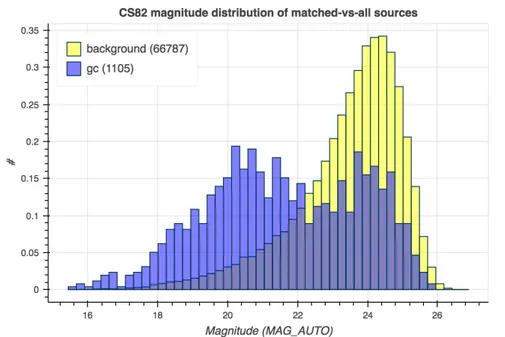
3.6 CS82 magnitude distribution of matched-vs-all sources . . . . 51
3.7 MAG_AUTO distribution for MLE cross-matched samples . . 52
3.8 SDS82 X-ray flux distribution of matched and non-matched sources . . . 52
3.9 SDS82 flux distributions for matched and non-matched sources 53 3.10 SDS82 distributions for matched and non-matched sources . . 53
4.2 Docker HEASoft container abstraction layers . . . 60
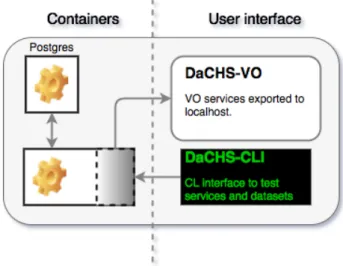
4.3 Docker-DaCHS containers interaction . . . 62
4.4 VERITAS processing workflow . . . 66
4.5 Assaisoftware design schema . . . 69
List of Tables
2.1 Swift-DeepSky x-ray energy bands . . . 17
2.2 Swift-DeepSky detected objects countrates . . . 24
2.3 Swift-DeepSky x-ray bands effective energy . . . 24
2.4 Swift-DeepSky detected objects fluxes . . . 25
3.1 Distribution of values in the SDS82 catalog. . . 35
3.2 Known blazars in SDS82 catalog. . . 36
3.3 VOU-Blazars candidates selection criteria . . . 37
3.4 VOU-Blazars candidates plot colors and symbols . . . 38
3.5 Catalogs (VO) used by VOU-Blazars . . . 39
Chapter 1
Introduction
Astrophysics lives its golden era of data, with multiple ground- and space-based instruments surveying the sky in all different wavelenghts – from gamma-rays, to X-gamma-rays, ultraviolet, optical, infrared, to radio band – as well as obser-vatories for astro-particles and gravitational waves brought astrophysics to a position of extreme wealth which we now need to work it out to extract the the best of knowledge from it to feed it back to the cycle of development.
To handle such plurality in data sets, computational infrastructure is a fundamental component of this discussion. Means to store, process and share data efficiently are critical to the mission of extracting and allowing others to analyze such data. Once data is being handled efficiently, the analysis of data through statistical and physical modeling is to be done with much more efficiency also.
Some efforts have been implemented in the last years to address the is-sue, the most prominent being the Virtual Observatories (VO), by the In-ternational Virtual Observatory Alliance (IVOA1). Most recently, the Open Universe initiative (OUN2) brought the discussion to the United Nations ar-guing that it is not only of the interest of the astronomical community but of the whole society to address this issue: on top of the VO achievements and individual solutions we, as a united society, organize a common agenda to effectively put in practice the well succeeded results and learn from each other – academia and industry – the failures.
The argument in place is about high-level data (also called science-ready data): easily accessible data, ready to be used for modelling and empirical inference. Data’s ultimate goal is to be used in its full extent, which in prac-tice it means to be frequently handled from various different perspectives. There are two major components under the high-level data discussion: the data itself – how comprehensive it is – and the software to handle it.
1http://www.ivoa.net/
To tackle the problem with a specific science case, we developed a pipeline to detect and measure x-ray sources from the Neil Gehrels Swift Observatory (former Swift Observatory, hereafter Swift) XRT instrument. The pipeline, called Swift DeepSky, handles all the processing from data download, de-tection and measurements, to data publication in the Virtual Observatory network if required by the user. After a basic set of input parameters, the pipeline delivers to the user a table of measurements ready for scientific use. As a science case, we applied the Swift DeepSky to the Stripe82 region, a prominent multi-wavelength field of the sky, in the search for blazars. Be-sides the pipeline, a set of software tools have been developed to access, correlate and publish data where we applied technical concepts we believe improve the everyday work we handle.
The work here presented has application in the Brazilian Science Data Center (BSDC), an infrastructure project started during this doctorate to de-velop the elements of high-level data. Together with the Open Universe ini-tiative, we are bringing the discussion here in place to the Brazilian society so that, in the near future, Brazil can not only become an important node in the astronomical data science network, but make this development a product for the society as a whole, beyond the academical walls.
The next sections of this introduction will present is some greater details the the elements this work builds upon and applies to: the scientific data ac-cess discussion and the Stripe82 data collection. Then, in the chapter ‘Swift DeepSky’ we describe the pipeline implemented and the production of the SDS82 catalog. The chapter ‘Brazilian Science Data Center’ presents the in-frastructure design and its implementation so far. Finally, in the conclusions, we summarise the work done.
1.1
Stripe 82
The Stripe82 is a 275 deg2 stripe along the celestial equator,−50 <RA <
60, −1.25 < Dec < 1.25 (≈ 1% of the sky), imaged more than 100 times as part of the Sloan Digital Sky Survey (SDSS) Supernovae Legacy survey (Annis et al., 2011; Abazajian and Survey, 2008). The name comes from SDSS’ sky survey plan, which cover the sky along stripes and that one is the 82 in the schema.
Repeated visits to the region created a collection in the archives of SDSS appealing to deep extragalactic studies, but by co-adding the Stripe82 images Annis et al. (2011) and Jiang et al. (2014) assembled a data set∼2 mag deeper
than the usual single pass data (magr ∼ 22.4) and with a median seeing of
≈ 1.1”, providing a unique field for the study of sensible objects like faint and distant quasars (Mao and Zhang, 2016).
The coverage strategy applied to the Stripe82 – considering also its partic-ular position in the Sky, being visible by telescopes in North and South hemi-spheres – made it particularly interesting for other observatories to follow-up. Stripe82 is emerging as the first of a new generation ofΩ ∼100 deg2 deep extragalactic survey fields, with an impressive array of multi-wavelength ob-servations already available or in progress. The wealth of multi-wavelength data in Stripe82 is unparalleled among extragalactic fields of comparable size. Besides dedicated surveys covering the Stripe, large area surveys cover the area in considerable extent: GALEX All-Sky Survey and Medium Imag-ing Survey (Martin et al., 2005) covered much of the field in the ultra-violet; UKIDSS (Lawrence et al., 2007) has targeted the Stripe as part of its Large Area Survey; parts of the Stripe82 are also in the footprint of FIRST, in the radio band.
At radio wavelengths, Hodge et al., 2011 provided a sources catalog con-taining ∼ 18K at 1.4GHz radio sources from observations of the Very Large Array with 1.8” spatial resolution. The catalog covers 92deg2of the Stripe82 down to 52µJy/beam, three times deeper than the previous, well known FIRST catalog (Becker, White, and Helfand, 1995) also covering the region.
Timlin et al., 2016 conducted deep infrared observations with the Spitzer Space Telescope in the Spitzer IRAC Equatorial Survey (SpIES), covering around one-third of the Stripe (∼115deg2) in 3.6 and 4.5µm bands, between−0.85 <
Dec < 0.85, −30 < RA < 35 and 13.9 < RA < 27.2, down to AB magni-tudes m3.6 =21.9 and m4.5 =22. SpIES provided 3 catalogs, for each
combi-nation of Spitzer-IRAC Channel-1 (3.6µm) and Channel-2 (4.5µm), each one providing more than∼ 6 million sources with spatial resolution better than (FWHM)∼2”.
In the far-infrared, Viero et al., 2013 observed the region with the Herschel Space Observatory SPIRE instrument to cover∼ 80deg2of the Stripe82 in the Herschel Stripe82 Survey (HerS). Observations go down to an average depth of 13, 12.9, 14.8 mJy/beam at 250, 350, 500µm, respectively. The band-merged catalog provided by HerS contains∼33000 sources.
High-resolution observations and deep sources catalog in optical was pro-vided by the CS82 collaboration (Soo et al., 2018; Charbonnier et al., 2017) us-ing the Canada-France-Hawaii Telescope coverus-ing∼170deg2of the Stripe down to magnitude mi =24.1 in the i-band with a 0.6” median seeing.
LaMassa et al., 2015 (see also LaMassa et al., 2012; LaMassa et al., 2013) combined Chandra archival data and new XMM-Newton observations to com-piled three source catalogs in X-ray (0.5< E(keV) < 10), covering∼31deg2, providing energy flux to a total of 6181 sources down to∼10−15erg s−1cm−2. Besides dedicated works to cover the Stripe82, a number of all-sky sur-veys of mapped either partially or entirely the region. The Dark Energy Sur-vey (DES) covered 200 deg2 down to magnitude mr ≈ 24.1 (()Abbott2018);
GALEX (Martin et al., 2005) observed 200 deg2 down to magnitude mNUV ≈
23; UKIDSS (Lawrence et al., 2007) covered the region in the infrared down to magnitude mJ ≈ 20.5; While (Lang2014) reprocessed WISE data to
pro-vide higher resolution coadded images. Figure 1.1 present the depths (in erg s−1cm−2) of the main surveys present to date covering the Stripe82 re-gion. The figure takes Timlin et al., 2016 (Table 2) as good summary of such list and considers also serendipitous reference the author crossed through.
FIGURE 1.1: Compilation of current surveys covering the
Stripe82, depth (in erg s−1cm−2) and observed waelengths
Multi-wavelength surveys are key to the study of Active Galactic Nuclei (AGN), as AGNs emit energy throughout the whole electromagnetic spec-trum. In particular to our interest, deep, multi-wavelength, wide-area sur-veys are key to the study of blazars.
To improve the Stripe82 data collections at the high energy range we cre-ated a deep x-ray catalog from the Neil Gehrels Swift Observatory observations, with data from the XRT instrument – 0.2 < E(keV) < 12. We designed a pipeline to combine all observations ever done by the Swift-XRT instrument (hereafter, Swift) to have the deepest catalog possible from Swift. We vis-ited every 120 Swift field and combined all observations overlapping in that field, detected and measured the flux in three independent wavebands: soft, medium, hard x-ray bands, besides the full band covering the entire energy range.
1.2
Blazars
The current paradigm for Active Galactic Nuclei (AGN) considers a cen-tral engine – a supermassive black hole (& 106M ) – being feed by a
sur-rounding accretion disk. Matter in the accretion disk comes from a thick torus, which is the structure delimiting the AGN food supply. Surround-ing this central engine there are clouds of dust more-or-less distant from the black hole which are perceived by spectral emission lines more-or-less broad. The clouds are would be trapped by the strong gravitational field and heated by the radiation coming out from the accretion disk while the matter (in the disk) is accelerated towards the black hole. In some objects we may observe a strong relativistic jet coming out from the central engine, roughly perpendic-ular to the disk; Such objects are called Radio-loud AGNs (Urry1995). Figure 1.2 offers a schematic view of such model.
FIGURE 1.2: Depending on the orientation between the ob-server and the AGN/galaxy different properties are observed. The Unified Model for AGNs states that different "types" of AGNs are effectively the result of which part of the system we are being able to observe. The figure presents a simple and clear view of observer’s point of view and type of object detected. Credit: GSFC/NASA Fermi collaboration website
(https://fermi.gsfc.nasa.gov/science/eteu/agn/)
Depending on the orientation relative to us of such system we will be able to observe different properties. For instance, if we are looking such system from the side (as in figure 1.2), the very central part and the accretion disk are going to be hidden by the torus, we should be able to see narrow emission
lines coming from the most distant clouds as well as both lobes (North/-South) from the relativistic jet in the Radio band.
In this model, blazars represent the fraction of AGNs with their jets aligned towards us – more precisely: at relatively small (.20−30°) angles to the line of sight. This produces strong amplification of the continuum emission ("rel-ativistic beaming") when viewed face-on. Radio-loud galaxies constitute a small fraction (∼ 10%) of the current known AGN population, around half of them are blazars (Padovani, 2017), making blazars a rare class of objects in our sky.
The blazar class includes flat-spectrum radio quasars (FSRQ) and BL Lac-ertae objects (BL Lac). The main difference between the two classes lies in their optical spectrum features: FSRQ presenting strong, broad emission lines supported by a non-thermal continuum, while BL Lacs present weak to no features at all, only the non-thermal continuum.
Blazars are characterized by emission of non-thermal radiation along a large spectral range, from radio to γ-rays, and possibly to ultra high ener-gies (Padovani et al., 2016). The overall Spectral Energy Distribution (SED, log(ν f(ν)) vs. log(ν) plane) of blazars is described by two humps, a
low-energy and a high-low-energy one. The peak of the low-low-energy hump can occur at widely different frequencies (νpeakS ), ranging from about ∼ 1012.5Hz (In-frared) to∼1018.5Hz (X-ray). The high-energy hump has a peak energy fre-quency somewhere at∼ 1020Hz to ∼ 1026Hz. Depending on the frequency of the low-energy hump BL Lacs can be divided in Low Synchrotron Peak (LSP or LBL) sources (νpeakS <1014Hz), Intermediate energy peak (ISP or IBL) sources (1014νSpeak < 1015Hz), or High energy peak (HSP or HBL) sources
(νSpeak > 1015Hz). Figure 1.3 (Padovani, 2017) present an schematic view of AGN – jetted and non-jetted – profiles. In the present picture, the first bump is associated with non-thermal emission from the Synchroton radiation, orig-inated from the jet’s relativistic charged particles moving in the magnetic field, while the second bump is understood as the result of low energy pho-tons that are Inverse Compton scattered to higher energies by the beam of relativistic particles.
Typically with continuous bolometric luminosity 1045 ∼1049erg/s, blazars are also known for displaying strong variability, with ν f(ν) variability up to
103−104times in timescales of weeks-to-days (0.01−0.001pc). In figures 1.4 and 1.5 present two examples of a LBL – the 3C279 blazar (Webb et al., 1990) – and a HBL – the Mrk421 blazar (Barres de Almeida et al., 2017) –, where we can visualy extrapolate the datapoints to see the low- and high-energy
FIGURE 1.3: Spectral Energy Distribution continuum compo-nents for jetted and non-jetted AGNs. Credit: Padovani, 2017.
FIGURE 1.4: Spectral Energy Distribution of 3C279, a LSP blazar
humps as well as their variability (figures created with ASDC SED tool3).
1.3
Data accessibility
Astrophysicists have been extremely successful during the last decades in designing observational facilities, collecting a wide range of signals with ever
FIGURE1.5: Spectral Energy Distribution of Markarian 421, a HSP blazar
more sensitivity, which boosted the number of publications – and ultimately, the knowledge – of the community as a whole. The amount and rate of data accumulation is, naturally, at its peak as we keep pushing technology speed and quality on data acquisition, soon projects like the LSST Robertson et al., 2017 will cross the rate mark of 10 TB (terabytes) per night. Plus, besides fresh new data arriving every day to active missions’ databases, a wealthy collection of past missions and data analysis results stored in institutes and universities across the globe, such data provides a unique temporal record of astrophysical events along the recent history of physics research.
Astronomical datasets are not only getting bigger, but also more complex. Multi-messenger astronomy is an emerging field of data analysis to relate as-tronomical events handled to us by different physical messengers: photons, gravitational waves, neutrinos, cosmic rays.
In such scenario, data accessibility becomes a crucial discussion (Wilkin-son et al., 2016). The main questions in place are (i) how to organize such diverse data collection in a meaningful way, (ii) how to publish the datasets clearly regarding their content, (iii) how to consume (i.e, query, analyze) such data. Ultimately, as scientists, we want to address the task: "query a dis-tributed petabyte-scale heterogeneous data base, build a sample of sensible data, ex-tract information"
As highlighted by Wilkinson et al. (2016), the data access discussion is not particular to astronomy, but most of science fields. And a good part of the issue is obviously because datasets are becoming bigger and bigger, but
mainly because we are moving to a new kind of publication media: from paper-format articles to digital documents. And this "simple" shift demands a whole new schema to make scientific resources available.
The astronomical community has organized itself to address the task a decade ago with the establishment of the International Virtual Observatory Alliance (IVOA4), and most recently the Open Universe initiative5is propos-ing to the United Nations an extension of this discussion to the benefit of not only the astronomical community but to the broader society.
1.3.1
The Brazilian Science Data Center
Aligned to the concepts about data accessibility, the Brazilian Science Data Center (BSDC) is a project started during this work with the ultimate goal to become a de facto interface – practical, useful, accessible interface – for the Brazilian community (not only, but primarily) to science-ready data. It is a project under construction at the Brazilian Center for Physics Research (CBPF) which builds upon the experience and is being developed in close collaboration with ASDC, the science data center of the Italian Space Agency (ASI), where the concept of a science-ready data center was originally ad-vanced. The BSDC shares on the ethos of and supports the Open Universe initiative and in this context is also supported by the Brazilian Space Agency (AEB).
The Open Universe6 is a recent initiative aimed at greatly expanding the availability and accessibility to space science data, extending the potential of scientific discovery to new participants in all parts of the world. The initia-tive was proposed by Italy and presented to the United Nations Committee on the Peaceful Uses of Outer Space (COPUOS) in June 2016. Open Universe guideline is to promote and create means to guarantee high-level space sci-ence data to be public and available by simple, transparent means so that a large part of the worldwide society can directly benefit from it. Not only scientist to be benefit, but also the general public through the educational of outer space data and data analysis tools. The ultimate goal is to boost the overall knowledge of society through all different uses of the data by pro-moting the inclusion of different groups, other than researchers only, in the appealing discussion of the observation of the Universe.
4http://www.ivoa.net/
5www.unoosa.org/oosa/en/oosadoc/data/documents/2016/aac.1052016crp/aac.1052016crp.6_0.html 6http://www.openuniverse.asi.it/
As the Open Universe initiative (OUN) is proposing the discussion at a global level, trying to address the different cultural and economical instances of society, the BSDC is going to address analogous contrast in social param-eters and continent-scale distances. Which brings BSDC and OUN to a very particular partnership where BSDC should provide practical, field results for theoretical discussions promoted by OUN.
The availability, accessibility and quality of data have an impact on all these groups, harnessing their potential and enabling them to enhance their contribution to the global stock of common knowledge. The moment is par-ticularly important as data storage, computing power and connectivity are broadly available to billions of people across all different scales, from su-percomputers to smartphones. At the same time the scope of human cultural and intellectual exchanges has broadened, as the current age of big data shar-ing and open source gathers pace.
It is well acknowledge today in the scientific community the benefits in productivity and innovation driven by open data access. However there is a considerable unevenness in the interfaces provided by outer space data providers. In the next years, considering the exponencial grow in overall data archives, both from the increase in capabilities to analyse existent data and by the new generation of observatories to come, it will be fundamental to the health of science to consolidate, standardize and expand services, pro-moting a significant inspirational data-driven surge in training, education and discovery.
From ever since the beginning of the Open Universe proposal to the United Nations, Brazil has been represented in the discussions through the active participation of BSDC members (Carlos H Brandt and Ulisses Barres, Almeida et al., 2017) in the various meetings held to discuss the initiative To sum-marise the theory, or foundations of the initiative, follows the digest of those meetings.
From Committee on the Peaceful Uses of Outer Space (2016):
The initiative intends to foster and spread the culture of space science and astronomy across different countries. It will pursue several interrelated tasks to the benefit of all actual and potential users of space science data, namely:
1. Promoting the robust provision and permanent preservation of science-ready data;
3. Fostering the development of new centralized services, both large and small, to exploit the interconnectedness of the mod-ern Intmod-ernet through new web-ready data;
4. Increasing web transparency to space science data;
5. Advocating the need for current and future projects to recog-nise the essential equality of hardware and software and in-corporate centralized high-specification end-to-end analytics into cost envelopes;
6. Promoting active engagement of the Committee on the Peace-ful Uses of Outer Space and other relevant national and in-ternational organizations towards tangible actions in this do-main.
Efforts to standardize and promote high-level data and data access ser-vices have been carried out in the last decades, among them the Interna-tional Virtual Observatory Alliance (IVOA), the InternaInterna-tional Planetary Data Alliance, the Planetary Data System of the National Aeronautics and Space Administration (NASA), the Virtual Solar Observatory and, with a focus on interdisciplinary standards, the Research Data Alliance. As a quite specific example – data file format – but also a very good one we can cite the FITS (Flexible Image Transport System) format which homogenized at great ex-tend the exchange and archival of data between individuals.
Open Universe wants to push the philosophy and all the experience ac-quired by the community in past and current efforts towards higher stan-dards in data services and transparency. Such effort is necessary in order to satisfy the needs of not only those target groups, but anyone interested in astronomy and space science. Space science data could be seen then not only as our magnificent participation in the Universe, but also a mean to pro-mote education and creativity across the Internet to whoever feels like doing it. It is then understood the importance to involve not only the astronomi-cal community but other stakeholders, so that efforts are not duplicated and experiences are shared to optimize both sides towards better data access.
In (Committee on the Peaceful Uses of Outer Space, 2018) it was expressed that the final calibrated data, together with complete ancillary data that char-acterize the observations, should be stored in online archives, following es-tablished standards, and that the data should be made available to the public, without the need of further data processing, after the required proprietary periods.
The Open Universe initiative, then, plains to engage with a wide user base, including the various target groups identified, ranging from the re-search community, higher and secondary education, citizen and amateur sci-entists, industry and other potential end users (Committee on the Peaceful Uses of Outer Space, 2017). The Brazilian Science Data Center, further pre-sented in section 4, is preparing itself to provide access to data, high-level software and a platform for the Brazilian and International community, and must focus to outreach the Brazilian society.
Virtual Observatory
The Virtual Observatory (VO) is a network of astronomical data collec-tions organised in so called services, distributed around the world. VO partic-ipants share the vision that astronomical datasets and other resources should work as a seamless whole. To that goal, the development of the various scien-tific and technological aspects to make VO possible is coordinated by the In-ternational Virtual Observatory Alliance (IVOA). IVOA is an open initiative for discussing and sharing VO ideas and technology, and body for promoting and publicizing the VO.
The Virtual Observatory program started in 2002 with the formation of IVOA with the National Virtual Observatory (from USA), the Astrophysical Virtual Observatory (from ESO) and the AstroGrid (from UK) as founding partners. The IVOA then grew to include other national projects and in-ternational organizations like the W3C (World-Wide Web Consortium) and the International Astronomical Union (IAU). From which (W3C) the work-ing structure was adopted and (IAU) standard recommendations could get support (Hanisch et al., 2015).
VO can be seen as a collection of resources, defined as (Hanisch, IVOA, and NVO, 2007) "VO elements that can be described in therms of who cu-rates or maintains it and which can be given a name and a unique identifier". In practice, the VO resources (or data services) are provided by data centers in a distributed configuration, worldwide. Each resource is published in a reg-istry, which has the role to broadcast the resources exist and their metadata. Much like the World Wide Web hyperlinks structure, this schema allows re-sources to be discoverable and, then, reachable by astronomers (Demleitner et al., 2014a; Demleitner et al., 2014b).
The figure 1.6 (Arviset, Gaudet, and IVOA, 2010) depicts the objective user interface on one side, the plural data archives on the other side and the VO standards and services in between.
FIGURE1.6: Virtual Observatory software resources harvesting infrastructure. Credit: (Arviset, Gaudet, and IVOA, 2010)
Key components of the VO infrastructure include the resources registry, the data access layer protocols and applications and application program-ming interfaces (API). On the data providers side there is a set of publish-ing registries that will communicate among them on sharpublish-ing resources and identifiers. A registry is a database of resource records – i.e, data collections descriptions and services metadata – in the VO. Figure 1.7, (Demleitner et al., 2014a), represent the data discovery activity involving registries and client applications.
On the user side, the client applications implement a generic interface to search the publishing registries, there is no central or preferential server they clients know about, but all the standard protocols in between the parts that abstract location and internal implementations. Which is to say that any application following the IVOA standards will integrate seamlessly to the network, as well as any data service, will be able to promptly publish and communicate in the network.
The underlying infrastructure, registries, data centers and databases, is transparent to the user. Astronomers will typically interrogate multiple ser-vices when searching for a particular kind of content. This is made possible by standardization of data models and exchange methods.
The formal products that IVOA provides to the community are standards establishing the interface between providers (e.g, services providing spec-tral data) and consumers (users applications) and among services themselves (e.g, harvesting resources). One of the policies during the process of devel-opment and eventual adoption of a new standard is to have two reference
FIGURE 1.7: Virtual Observatory resources harvesting infras-tructure. Credit: Demleitner et al., 2014a
implementations to it. The objective of such policy is to ensure that the stan-dard can effectively work and that its application is useful to the research community.
The standards released or under discussion by IVOA are available at http://www.ivoa.net/documents/index.html. Each recommendation docu-ment goes through a cycle of discussions where description goes to the de-tails to allow a better implementation and fulfill the compatibility space. It is not IVOA’s mission to provide the software, only the standards. Neverthe-less, the Alliance do publish the list of software developed by the community in the VO framework:
http://www.ivoa.net/astronomers/applications.html.
During this thesis we used the server-side data publication package de-veloped by the German Astronomical Virtual Observatory (GAVO) DaCHS (Demleitner et al., 2014b). And, to the client-side, we implemented tools to handle VO data collections and services discovery.
Chapter 2
Swift DeepSky project
The amount of time a telescope observe a particular region of the sky dictates the amount of information that can be retrieved from that particu-lar region. An astonishing demonstration of the power of extended integra-tion time was given by the Hubble Space Telescope in 1995; the telescope observed a small region of the sky for 10 consecutive days generating more than 300 images, which were then combined into what was called the Hubble Deep Field, the deepest observation done to that date.
Objects with apparent luminosity too low to be significantly detected in a single exposure may show out when many observations are co-added. Clearly, co-addition is possible only when the telescope has visited a given region of the sky multiple times, which happens in three situations: (i) the ob-served region is signed to a series of dedicated time project, like the Hubble Deep Field, (ii) the region is part of a wide field survey footprint periodically visited, as in the Sloan Digital Sky Survey, or (iii) the telescope has long been collecting data that overlaps become a feature, which is the scenario we are exploring with the Swift Telescope.
Swift primary goal is to investigate Gamma-Ray Bursts (GRB), the tele-scope carries three detectors: the Burst Alert Teletele-scope (BAT1), which trig-gers the whole telescope’s attention whenever a GRB is detected; the X-Ray Telescope (XRT,2), that follows the subsequent emission of the GRB; fi-nally the UltraViolet-Optical Telescope (UVOT3) responsible for registering the uv/optical GRB afterglow. Although its priority is GRB events, Swift will follow a schedule of observations of x-ray sources whenever GRBs are not on the sight.
Willing to create the deepest catalog of Swift X-ray data that could be dy-namically updated whenever new observations arrived, we developed the
1https://swift.gsfc.nasa.gov/about_swift/bat_desc.html 2https://swift.gsfc.nasa.gov/about_swift/xrt_desc.html 3https://swift.gsfc.nasa.gov/about_swift/uvot_desc.html
Swift-DeepSky pipeline. The pipeline will combine all observations taken by Swift with its XRT instrument in Photon-Count mode since it started operat-ing, in 2004. The co-added image will be used to detect X-ray sources in the field and then proceed with a series of flux measurements (countrates and
νFνfluxes).
For the first 7 years of Swift operation, from 2005 to 2011, D’Elia et al. (2013) provided the 1SWXRT with positions and flux measurements for all point-like sources detected in XRT Photon-Count mode observations with exposure time longer than 500seconds. While Evans et al. (2013) published the1SXPS catalog with ∼150k sources from all observations made by Swift-XRT during its first 8 years of operation.
The Swift-DeepSky goes one step further by providing the software – open source, clearly – and a mechanism to have a central, VO-compliant catalog of the DeepSky measurements keeps an up-to-date version of itself, forever – until Swift finishes its lifetime. This work combines both methodologies – D’Elia et al.; Evans et al. – for XRT data reduction in a steady, scalable software solution where software design is a major component of this work results.
Rational
The pipeline is the implementation of a conceptual solution for high-level user interface for scientific pipelines. We bring in collection cutting edge tech-nologies to provide secure, fully automated data analysis software to address also non-technical users, besides providing results producibility, which we believe to be an obstacle for science development. The goal of the DeepSky is to deliver a reliable and stable Swift-XRT data reduction tool at the same time that it keeps a living catalog of such data, that grows and updates itself at each use.
The pipeline combines all Swift XRT events observed in Photon Count mode in observations longer than 100 seconds in a region of 120 around a given position of the Sky. HEASoft4 tools are used to combine multiple ob-servations and extract physical information from the objects observed. The detection of source are done using theFull bandpass, 0.3-10 keV. We then measure the photon flux of each detected source using HEASoft Sosta in three intervals: Soft (0.3-1 keV), Medium (1-2 keV), Hard (2-10 keV). When-ever a source is not identified in one of the bands, an upper limit is estimated using the local background level and effective exposure time. Energy fluxes
(νFν) are corrected after our galaxy absorption, considering Milky-Way’s
hy-drogen column (NH) in the line-of-sight to the source and a spectral slope con-sidering instrumentation effects. At the end of the processing, the pipeline may upload the outputs to a central server where the results will be merged to the Swift-DeepSky primary sources catalog.
We applied the pipeline to the entire region covered by the Stripe82 and generated a unique deep x-ray sources catalog for the region. For the sake of clarity and to eventually motivate the reader in using DeepSky , the process of efficiently surveying a region of the sky, the steps of such processing are explained in details as well as supportive tools are equally made public.
In the next sections we describe the DeepSky pipeline work-flow in its technical aspects as well as the methodology on surveying a large area of the sky to generate a catalog of unique sources. To the technological aspect of the work, we will also present the software design and infra-structure adopted to the publication of the DeepSky pipeline.
2.1
The pipeline
DeepSky combines all Swift-XRT observations for a given region of the sky. The region is defined by a central coordinate and a radius. The pipeline combines all events and exposure-maps centered in the corresponding field and detect the objects using all events in the XRT energy range – 0.3-10 keV. For each object detected, the pipeline then do a series of flux measurements in three energy sub-ranges and Swift’s full energy band:
Band Energy range (keV)
Full 0.3 - 10 keV
Soft 0.3 - 1 keV
Medium 1 - 2 keV
Hard 2 - 10 keV
TABLE2.1: Swift-DeepSky x-ray energy bands
2.1.1
Processing stages
Figure 2.1 presents the DeepSky pipeline workflow, it is composed by six conceptual blocks. The user provides a position on the Sky – Right Ascen-sion and Declination –, optionally a radius defining the surrounding region of interest (default is R = 120), and the pipeline will proceed through the following steps:
1. Search for Swift observations in that region 2. Combine (textiti.e, co-add) all observations 3. Detect objects using all events (0.3 < E(keV) < 10)
4. Measure each object fluxes (in three x-ray bands) 5. Estimate spectral energy slope
6. Convert count rates to νFν (νFν) flux
At the end of the processing the pipeline outputs the flux measurements in two sibling tables (i.e, same number of objects, respecting the same order) containing (i) photon fluxes and (ii) νFν energy fluxes. Provides also the
x-ray events image with each detected object labeled and the corresponding exposure-map for visual inspection. As well as important for the sake of transparency, all temporary files used during the processing are kept in a separated folder.
Swift observations
The Swift Master Table5 is the record table of all Swift observations, it contains informations like central coordinates (RA,Dec), start and end time-stamp, instrument used (BAT, XRT, UVOT), observation mode (PC, WT), unique observation identifier, for each observation done by the satellite. This table, maintained by the Swift data center, is where the pipeline starts.
The pipeline starts by querying the Master Table for observations done by the Swift-XRT telescope in Photon Counting6 mode in a given region of the sky. The region is defined by the user through an (RA,Dec) position of the sky and a radius to consider: all observations with (central) coordinates within the the region will be evaluated. The pipeline offers a default radius value of 120since this is Swift-XRT field-of-view, meaning that the position of interest for the user may have been covered by any observation within 120.
In practical terms, the pipeline starts with a pair of coordinates or object name of interest – in that case, DeepSky will ask CDS/SIMBAD7 for the cor-responding (RA ,DEC ) position:
# swift_deepsky --object GRB151001A
5https://heasarc.gsfc.nasa.gov/W3Browse/swift/swiftmastr.html 6http://www.swift.ac.uk/analysis/xrt/modes.php
Once the list of observations potentially covering the given position is retrieved, the respective data is downloaded from the Italian Swift Archive8. The pipeline uses the archived level-2 data, in particular level-2PC event-files (OBSID/xrt/event/*pc*) and exposure-maps (OBSID/xrt/products/*pc_ex*).
FIGURE2.2: Swift XRT observation images example
Combining observations
With all event-files and exposure-maps in hands we combine them to build one unique events-file and exposures-map. We first use HEASoft Xs-elect9 to extract all events in good time intervals from each observation and
8http://www.ssdc.asi.it/mmia/index.php?mission=swiftmastr 9https://heasarc.gsfc.nasa.gov/ftools/xselect/
write them all in one list of events. Analogously, HEASoft Ximage10 is used to sum each observation’s exposure-map.
At this point we have the two files – events list and exposures-map – that will be used for the rest of the pipeline.
FIGURE2.3: Swift XRT combined observations image example
Objects detection
Objects detection are done considering all events registered by Swift-XRT, in theFull (XRT) energy range – 0.3−10keV. HEASoft XImage’sdetect rou-tine is used for sources identification, background and countrates estimates.
Thedetect algorithm estimates the image background from a set of small boxes across the image. After a sliding-cell traversed the field looking for excesses, the objects are detected in a boxes of size such that its signal-to-noise ratio is optimized. When we initialize the events and exposure images indetect we define a an area of 800-x-800 pixels in the image, which repre-sent ∼ 160 on the sky. The size was chosen arbitrarily to respect Swift XRT field of view (120) and include extra field of the sky, but not still keep it at a minimum because of performance (the process of combining the images is computationally expensive and scaled with the image size).
In figure 2.4 we see the objects detected in our example case. We can compare this figure to those in figure panel 2.2 to see how the detections may change. These – from the combined image – are the detected sources we will carry for the next steps of the pipeline.
To illustrate how detection results are given by detect, it is presented below the photon flux estimates given by the routine:
FIGURE2.4: Swift XRT combined observations detection exam-ple
! Field Name : GRB151001A ! Instrument : SWIFT XRT ! No of sources : 4 ! Exposure (sec) : 8763.0135 ! Input file : GRB151001A_sum.evt ! Image zoom : 1.0000
! Back/orig-pix/s: 8.6523602E-07 ! Equinox : 2000 ! RA Image Center: 233.73870 ! Dec Image Center: 10.972480 ! Start Time : 2015-10-01T15:05:48.00 ! End Time : 2015-10-02T02:07:39.00
! # count/s err pixel Exp RA(2000) Dec(2000) Err H-Box
! x y corr rad (sec) prob snr
1 2.03E-01+/-5.2E-03 514.05896 491.67648 8374.13 15 34 55.118 +10 58 00.128 -1 72 0.000E+00 3.940E+01 2 1.43E-03+/-5.3E-04 655.42859 462.85715 8755.90 15 34 32.489 +10 56 52.130 -1 15 5.746E-06 2.669E+00 3 2.39E-03+/-7.3E-04 354.76923 683.92310 8089.25 15 35 20.626 +11 05 33.257 -1 18 1.445E-08 3.302E+00 4 1.37E-03+/-5.7E-04 631.57141 725.14288 8758.83 15 34 36.296 +11 07 10.435 -1 15 7.914E-05 2.426E+00
Flux measurement
After the detection of objects using all events collected, we then re-use detect considering only the events in the Soft , Medium , Hard energy range. We do so to estimate the background at each band, which will be used in the next step to estimate each object’s signal (photon counts) using another algorithm.
The combined list of events appear at each x-ray band as shown in the figure panel 2.5
Photon flux measurement
Using the background measurements in each band and the detected ob-jects positions we now will measure the corresponding photon fluxes using
(A)Full (B)Soft
(C)Medium (D)Hard
FIGURE2.5: Swift XRT combined observations per-band exam-ple
XImage’ssosta tool.
Sosta measures objects count rates weighted by the exposure map pre-viously created, and the background prepre-viously computed by detect. It is worth to remember that objects –and their corresponding position – were de-tected using the full energy band, and background measurements in each band.
For each (object) position Sosta consider the events within a small region around it. The region is dynamically defined by the amount of encircled energy fraction (eef), which is a given parameter defined by the pipeline based on the detect-estimated intensity.
When the events accounted do not result in significant statistics to result in a flux measurement, an upper limit estimate is provided when sufficient photons can not be associated to the sources, the background (noise) level and the exposure time. The upper limit estimates, flux measurements and, together with the exposure times, all those values populate our output files. Table 2.2 presents what are the measured results for our example.
Column name Source 1 Source 2 Source 3 Source 4
RA 15:34:55.118 15:34:32.489 15:35:20.626 15:34:36.296
DEC +10:58:00.128 +10:56:52.130 +11:05:33.257 +11:07:10.435
countrates [0.3-10keV] 2.030E-01 1.430E-03 2.390E-03 1.370E-03
countrates error [0.3-10keV] 5.200E-03 5.300E-04 7.300E-04 5.700E-04
exposure-time(s) 8374.1 8755.9 8089.2 8758.8
countrates [0.3-1keV] 7.120E-02 4.086E-04 7.964E-04 4.565E-04
countrates error [0.3-1keV] 3.102E-03 2.863E-04 4.247E-04 -5.694E-01
upper limit [0.3-1keV] -999 -999 -999 1.291E-03
countrates [1-2keV] 7.195E-02 4.086E-04 5.311E-04 3.044E-04
countrates error [1-2keV] 3.102E-03 2.863E-04 3.451E-04 -5.694E-01
upper limit [1-2keV] -999 -999 -999 1.291E-03
countrates [2-10keV] 5.986E-02 6.129E-04 1.062E-03 1.370E-03
countrates error [2-10keV] 2.828E-03 3.472E-04 4.911E-04 5.700E-04
upper limit [2-10keV] -999 -999 -999 -999
TABLE2.2: Swift-DeepSky detected objects countrates
Energy flux measurements
At the last measurement stage the pipeline transforms photon flux to en-ergy νFνflux, the integrated flux at a pre-defined effective frequency in each
band. To compute the νFν flux we have to estimate spectral slope for each
source across the energy band. The final energy fluxes are then corrected by our galaxy’s absorption.
For each energy band, the effective frequency is defined as: Band Effective energy (keV)
Full 3 keV
Soft 0.5 keV
Medium 1.5 keV
Hard 4.5 keV
TABLE2.3: Swift-DeepSky x-ray bands effective energy
The amount of dust absorbing x-ray light is computed using HEASoft NHtool, which estimates the density of Hydrogen atoms column along the line of sight for each source.
Based on theNHvalue, the count rates between Soft + Medium (combined) andHard bands, and Swift-XRT instrument sensitivity in each band, the spec-tral slope is calculated. With the energy slope in hands, each source has its countrates measurement transformed to energy νFνflux in erg/s/cm2. In
Column name Source 1 Source 2 Source 3 Source 4
RA 15:34:55.118 15:34:32.489 15:35:20.626 15:34:36.296
DEC +10:58:00.128 +10:56:52.130 +11:05:33.257 +11:07:10.435
NH 3.11E+20 3.08E+20 3.19E+20 3.13E+20
energy-slope 0.734 0.8 0.8 0.8
energy-slope error +0.04/-0.04 -999/-999 -999/-999 -999/-999
exposure-time 8374.1 8755.9 8089.2 8758.8
nufnu [3keV] 2.97984e-12 1.98813e-14 3.33525e-14 1.90786e-14 nufnu error [3keV] 7.63308e-14 7.36859e-15 1.01871e-14 7.93782e-15 nufnu [0.5keV] 1.75878e-12 1.02097e-14 2.00685e-14 1.14504e-14 nufnu error [0.5keV] 7.66256e-14 7.15378e-15 1.0702e-14 -1.42823e-11
upper limit [0.5keV] -999 -999 -999 3.23822e-14
nufnu [1.5keV] 2.57653e-12 1.45474e-14 1.89332e-14 1.08439e-14 nufnu error [1.5keV] 1.11083e-13 1.01931e-14 1.23025e-14 -2.02843e-11
upper limit [1.5keV] -999 -999 -999 4.59906e-14
nufnu [4.5keV] 3.28326e-12 3.30378e-14 5.72567e-14 7.38553e-14 nufnu error [4.5keV] 1.55113e-13 1.87155e-14 2.64772e-14 3.07281e-14
upper limit [4.5keV] -999 -999 -999 -999
TABLE2.4: Swift-DeepSky detected objects fluxes
2.1.2
Results
The pipeline primary output are the countrates and νFν flux tables, like
tables 2.2 and 2.4 previously exemplified (except that here, in this document, they are transposed to properly fit the page width). The fluxes, respective error and upper limits are provided for the all bands –Soft , Medium , Hard – as well as the Full band. Total exposure time, spectral energy slope and hydrogen column density (NH) are also included.
Besides the flux tables, the combined exposure-map and events-file in FITS format – suitable for further analysis – and their.gif versions, as well as the log file with each processing steps information. All provided for the sake of complete transparency easy access and visual inspection whenever required. Are also provided in the output directory, properly encapsulated in a (tarball) file "tmp.tgz", all the intermediate files used during the processing. Which allows the user to control every step of the pipeline and eventually double check the results.
2.2
Creating a living catalog
In accordance to our science-ready and high-level services guidelines we have implemented anupload option to the DeepSky pipeline to allow results to be shared as soon as they are produced, transparently, to a worldwide
audience. The idea to have the public, VO-compliant catalog always up-do-date, the updates made by the users themselves on demand. Eventually, the whole sky Swift DeepSky database will be available, again, up-to-date by the users worldwide.
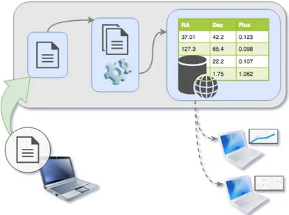
Figure 2.6 depicts the flow of results, from the user that generated the last results, to our servers, back to the users through a VO service and online table.
FIGURE 2.6: Workflow of the DeepSky living catalog: an user runs the pipeline to a specific region of their interest, results are transparently uploaded to a dedicated server where they are combined with existing table. The VO-compliant catalog then exposes the updated catalog, publicly available to other users
The upload of the pipeline output is done anonymously and explicitly under the user request (through the explicit use of--upload argument).
The output files are compressed and securely uploaded to a dedicated server. When the output files arrive to the server, they verified against the already existing database of previous results to verify for duplicates. If a par-ticular source is already in the published results to parameters are compared between them: total exposure time and full-band flux measured; If the cor-responding values are greater in the recently arrived data, then the database is updated to include (and substitute) the new measurements, otherwise the left unchanged. If the new data is not a duplication, it is simply included in the database.
2.3
Surveying the Stripe82
In this section we describe the process of covering a large contiguous re-gion of the sky with discrete steps in the RA,Dec plane. We will do so for the Stripe82 field, used for the creation of our SwiftDS-82 catalog. We will go through the following steps:
• define the coordinates to visit and coverage area (pointings); • define an efficient way to process all pointings;
• aggregate the results to compile a unique catalog.
Mapping the sky with HEALpix
The region coverage task is basically the classical optimization problem of covering a rectangular area with circles in such a way that there is no gaps in between the circles and a minimal overlapping area between the circles.
Clearly we want to completely cover the region of interest, but the opti-mization regarding the overlapping area is not of major concern. It is impor-tant to define a methodology to avoid redundant processing so that compu-tational resources are used wisely, but some overlapping excess of overlap-ping is actually required to compensate for Swift’s square images and non-uniform coverage.
We have chosen to use Healpix tesselation schema as it provides the mech-anism to define a regularly spaced coordinates grid. The schema defined is multi-dimensional tree-like structure where at each level there will be 12+
2level+1non-overlapping cells covering the sky. At each level, HEALpix grid cells –called diamonds– have an equal area.
Notice that at each level the grid cells have a pdefined size, which re-duces approximately by half at each level up. The factor two –like in a Quad-tree– comes from each diamonds being split in four each time we go one level up. Another important characteristic about HEALpix schema is in its cells positioning: the coordinates system is fixed; meaning that a position in the sky will always be represented by the same HEALpix element in a given resolution (level), independent of the surrounding data or platform in use.
The software implemented for this task is published as a small package called moca, it is based in healpy and inspired by mocpy. The package pro-vides an interactive document in itsdocs folder for reference.
To build our list of pointings we queried the Swift Master table for all ob-servations inside the Stripe82 region -60 < RA(deg) < 60 and -1.25 < Dec(deg)
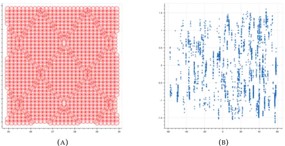
(A) (B)
FIGURE2.7: HEALPix pointings map example when covering a hypothetical contiguous region (A) and the representation of
the Swift observations over the Stripe82 (B).
< 1.5. Each position observed by Swift is associated to a Healpix element, at a given level. Duplicated elements are not considered as our goal here is to de-fine (unique) positions to visit. When all observations have been associated to its respective Healpix element, the inverse transform – i.e, from Healpix elements to coordinates – is taken to build up the list of pointings to collect data from.
The Healpix level is defined based on Swift XRT field-of-view. Since we want to completely cover the region, the steps between our pointings cannot be bigger than our observations field-of-view. Swift XRT has a FoV of 120, Healpix levels 9 and 8 provide pixels with sizes 6.870and 13.740, respectively. For our purpose, since we better have extra overlap than gaps, level 9 is the appropriate level to used when defining the pointings.
When calling the pipeline with the positions from this process and the original radius from Swift-XRT FoV – 120–, adjacent pointings will overlap. Although this is not optimal from the processing point-of-view, it is neces-sary to guarantee our results the best signal-to-noise by combining all possi-ble events in that area.
Figure 2.7a illustrates the coverage of a small region following the algo-rithm described above. And figure 2.7b presents all pointings defined to run DeepSky over.
The resulting list of pointings contains 699 entries, from ~7000 observa-tions. Now that we have the list of positions we want to visit, we have to
define how we will do it, considering that the processing of ~7000 observa-tions is a quite time consuming task.
Parallel running the pipeline
Covering the Stripe82 ∼ 700 pointings were defined, and since they are all independent from each other we may use a parallel strategy to reduce the amount of real time consumed. I will also take the chance to present the software packaging adopted, which makes the setup and parallel run a straightforward process.
Each pointing is processed independently of other runs. Such indepen-dence between the runs makes place to a simple parallelism strategy known as bag of tasks: a set of independent jobs, homogeneous or not, that may run in parallel in a FIFO (first in, first out) queue structure.
In the of DeepSky , the most demanding computational resource is CPU, memory, disk and network I/O present modest use. CPU bottleneck is good because it is an easy to acquire and easy to control resource.
To control the execution of these∼ 700 jobs a easily portable queue sys-tem was implemented. It implements a FIFO queue syssys-tem to which the user input a list of tasks to run and the number N of maximum running jobs al-lowed. The queue system then will keepN running jobs, feeding the next in the waiting line, until all (700, for instance) jobs have been completed.
The queue system used was implemented usingBash scripting and may be downloaded from Github, Simplest-Ever-Queue system. Many queue sys-tems are publicly available, but none of them is simple enough to just use; they all need more-or-less complex setups and they are usually focused on larger, distributed high performance systems. My goal was to provide a sim-ple queue system that anyone with access to a multiprocessor machine could use it effortlessly.
Aggregating the results
Each successful run of the DeepSky pipeline will output a set of catalogs, images, log files, etc. Of major interest are the catalogs – photon and energy flux catalogs –, containing measurements for each detected object.
When multiple different runs share an overlapping area and objects are detected in such region we will end with multiple sets of measurements from the same object. From the multiple runs, to have a unique list of sources we
have then to clean out the duplicates. In this Stripe82 processing, concate-nating the output of all ~700 runs will generate one big table with inevitably many duplicates.
The removal of duplicated objects is done through a cross-matching, where we basically search for objects that are too close to be two different sources. The definition of this confusion distance is usually associated with the instru-ment’s point spread function, at least the PSF is a good first approach since a point source will not be better defined than that. Whenever two (or more) objects follow within this tolerance distance one of them is kept and other(s) are discarded.
Objects within the confusion distance are filtered after their Full band signal-to-noise ratio (SNR): the entry with higher SNR is set as the primary source and goes to the final catalog of unique sources.
Finally, the Swift-DeepSky over Stripe82 produced a flux catalog with 2755 (unique) sources. In the next section we will look some properties of this final catalog.
2.3.1
Checking the results
The 1SXPS catalog (Evans et al., 2013) provide an all-sky deep view of the Swift-XRT sky using the first 8 years of observations. That work took a different approach, using data from XRT’s Window Timing (WT) mode to investigate variability also, but one of their results is an integrated flux like we have done in this work.
To check how our results compare to (Evans et al., 2013) we cross-matched the catalogs to a distance of 5”, which is the average position error in the 1SXPS. Figures 2.8a and 2.8b present the countrates (flux) distribution side-by-side where we see the catalogs mostly agree, 1SXPS apparently showing an excess in faint sources. A more qualitative visualization of that compari-son though may be seen in figures 2.9a and 2.9b, where we see SDS82 recov-ering more photons from objects, naturally as exposure time is bigger, and in overall agreement with their results.
2.4
Pipeline distribution
The pipeline is publicly available and maintained as an open source project. It is distributed using a novel software technology, where the concept of soft-ware portability is implemented at its highest level.
(A) Histogram (B) Violin-plot
FIGURE2.8: Countrates distribution (ct/s-1) of catalogs SDS82 and 1SXPS, figure (A) presents the well-known histogram view where we can see the distributions overlap, while figure (B) of-fers a violin-plot where we see individual distributions density.
(A) Cumulative Distribution (B) Scatter plot
FIGURE2.9: Countrates comparative plots SDS82 vs 1SXPS
Many concepts may characterise a software, portability is the one that qualifies whether a software can run in different platforms. A non-portable software is one that runs in one, specific operating system or architecture (i.e, platform); on the other hand, a portable software may run in different platforms.
Regarding portability, in very recent years the landscape of computing has been significantly changed with the development of linux containers11. Con-tainers are the top level of virtualisation technologies, which allows us to
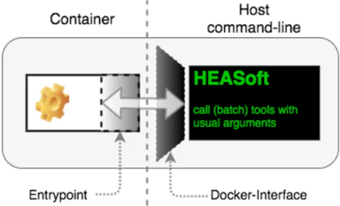
mimic an entire environment around a software so that the bare system un-derneath it can be highly abstracted. This paradigm removes the weight of portability from the (core) software, which not only simplifies the develop-ment but also promotes the focus on developing core functionalities for the software. In Section 4.1.1 we go in some deeper details about Containers, in particular their implementation interface Docker (containers).
The DeepSky pipeline is distributed in a (Docker12) container, which pro-vides the user a ready-to-use software package. Everything necessary for the pipeline to run is packaged together – including the HEASoft tools. And the package will run in any platform, although it has been developed for linux systems, because of the virtualisation framework Docker provides, im-plemented a very efficient abstraction layer between Windows and MacOS systems to make use of Linux containers.
By using such technology and a public code base, we address the portabil-ity or transparency issues about reproducibilportabil-ity of scientific results. Another aspect we care about is that of productivity: the use of containers allow the users of this package to spend virtually zero time in setting it up, ready for science.
Chapter 3
The SDS82 catalog
Swift-DeepSky outputs a table with the measured fluxes (νFν fluxes and
countrates) in the Full band, Soft , Medium and Hard . In the Stripe82 region, these catalog contain 2755 unique sources. The flux catalog provides also total exposure time, energy slope, and NH used during the conversion from countrates to νFνflux.
The catalog reaches 5σ flux limits of 4.04×10⁻¹⁵, 4.96×10⁻¹⁶, 1.20×
10−15 and 7.67×10⁻¹⁶ erg.s−1.cm−2 in the Full , Soft , Medium , Hard , respectively (figure 3.1). Table 3.1 summarizes the numbers of the catalog.
FIGURE3.1: SDS82 νFνfluxes distribution
While figure 3.2 presents the sensitivity of the catalog from a different perspective by showing the Full band countrates behavior along the total
exposure time.
FIGURE3.2: SDS Countrates vs Exposure time
The SDS82 catalog is available through the Virtual Observatories network as well as BSDC’s VO website1.
3.1
Blazars in SDS82
The search for blazars is a particular application for Swift-DeepSky data at it may help to reveal distant objects non detected previously by other, shal-lower studies. Particularly interesting for high energy studies is the class of High Synchrotron Peak (HSP) blazars as they are among the most energetic objects in the Universe emitting photons beyond TeV.
In the SDS82 footprint there are 33 known 5BZCAT (Massaro et al., 2015) blazars, of which 17 are known to be HSP sources (Chang and Giommi, in preparation). Table 3.2 lists these known blazars together with there desig-nation in BZCAT and HSP catalogs.
We then applied the VOU-Blazars tool to search for new blazars in SDS82 sources.