NMR measurements for hazelnuts classification

NMR measurements for hazelnuts

classification

Unione Europea UNIVERSITÀ DEGLI STUDI DI SALERNO

FONDO SOCIALE EUROPEO

Programma Operativo Nazionale 2000/2006

“Ricerca Scientifica, Sviluppo Tecnologico, Alta Formazione” Regioni dell’Obiettivo 1 – Misura III.4

“Formazione superiore ed universitaria”

Department of Industrial Engineering

Ph.D. Course in Industrial Engineering

(XVI Cycle-New Series, XXX Cycle)

NMR measurements for hazelnuts classification

Supervisor

Ph.D. student

Prof. Consolatina Liguori

Domenico Di Caro

Ph.D. Course Coordinator

Prof. Ernesto Reverchon

Publications resulting from

this work

Di Caro, D., Liguori, C., Pietrosanto, A. and Sommella, P., 2016, May. Investigation of the NMR techniques to detect hidden defects in hazelnuts. In Instrumentation and Measurement Technology Conference Proceedings (I2MTC), 2016 IEEE International (pp. 1-5). IEEE.

Di Caro, D.; Liguori, C.; Pietrosanto, A.; Sommella, P.; Gibboni, A. (2016). UTILIZZO DI TECNICHE DI RISONANZA MAGNETICA PER IL RILIEVO DI DIFETTI OCCULTI NELLE NOCCIOLE. In: Atti del XXXIII Congresso Nazionale dell’Associazione GRUPPO MISURE ELETTRICHE ED ELETTRONICHE Benevento 19-21 settembre 2016 Vol.1, Pag.31-32

Di Caro, D., Liguori, C., Pietrosanto, A. and Sommella, P., 2017. Hazelnut Oil Classification by NMR Techniques. IEEE Transactions on

Instrumentation and Measurement, 66(5), pp.928-934.

Di Caro, D., Liguori, C., Pietrosanto, A. and Sommella, P., 2017, May. Using a SVD-based algorithm for T 2 spectrum calculation in TD-NMR application to detect hidden defects in hazelnuts. In Instrumentation and Measurement

Technology Conference (I2MTC), 2017 IEEE International (pp. 1-6). IEEE.

Di Caro, D.; Liguori, C.; Pietrosanto, A.; Sommella, P.; Gibboni, A. (2017). CLASSIFICATION OF HAZELNUTS IN SHELL BY MEANS OF TD-NMR TECHNIQUES. In: Atti del I Forum Nazionale delle Misure, Modena 14-16 Settembre 2017, Pag.125-126

Di Caro, D., Liguori, C., Pietrosanto, A. and Sommella, P., 2018, May. Advanced TD-NMR based estimation of the inshell hazelnuts quality parameters. In Instrumentation and Measurement Technology Conference

Contents

Contents... I List of figures ... IV List of tables ... VII Abstract ... VIII Introduction ... IX

Chapter I ... 1

Quality control in hazelnuts processing ... 1

I.1 Main properties and hidden defects of the hazelnuts ... 1

I.2 Techniques to detect hazelnuts quality ... 3

I.3 Nondestructive techniques in food quality control ... 4

I.4 Using NMR in food quality control ... 5

Chapter II ... 9

NMR methods and equipment... 9

II.1 NMR Theory ... 9 II.2 NMR equipment ... 11 II.2.1 Magnet ... 12 II.2.2 Probe ... 12 II.2.3 Transmitter ... 13 II.2.3 Receiver ... 14 II.3 NMR methods ... 16

II.3.1 Single pulse sequence ... 17

II.3.1 CPMG sequence ... 20

II.4 The adopted TD-NMR measurement system ... 22

II.4.2 Magnet and probe ... 23

II.4.3 Personal computer ... 26

II.5 Influence parameters in liquid and solid samples ... 26

II.5.1 Temperature controller ... 27

II.5.2 Other influence parameters ... 28

Chapter III ... 31

Hazelnut oil characterization ... 31

III.1 Instrumental parameters ... 31

III.2 CPMG setup ... 33

III.3 Echo response pre-processing ... 33

III.3.1 Mean value ... 35

III.3.2 FFT magnitude ... 36

III.3.3 Polynomial regression ... 37

III.3.4 Comparison among the three methods ... 38

III.4 Study of the echo decay envelope ... 39

III.4.1 ES parameter ... 40

III.4.2 Multi-exponential approximation ... 40

III.5 Experimental results on oil samples ... 42

III.5.1 Sample preparation ... 42

III.5.2 Experimental results ... 42

Chapter IV ... 51

In-shell hazelnuts characterization ... 51

IV.1 CPMG sequence ... 52

IV.2 Moisture content evaluation ... 53

IV-3 Kernel development evaluation ... 56

IV-4 T2 distribution calculation using the SVD algorithm ... 59

IV-5 T2 distribution ... 60

Chapter V ... 63

Classification algorithm ... 63

V.1 Moisture content evaluation ... 64

V.2 Kernel development evaluation ... 66

V.3.1 Unhealthy hazelnuts not completely developed ... 68

V.3.2 Unhealthy hazelnuts completely developed ... 69

V.3.3 Threshold setting by means of ROC curve analysis ... 71

V.3.4 Threshold validation using a bootstrap method ... 74

V.4 Analysis of the algorithms execution time ... 76

Chapter VI ... 79

Conclusions ... 79

References ... 81

Appendix ... 87

List of figures

Chapter I: Quality control in hazelnuts processing

Figure I-1……….2

Figure I.2……….6

Chapter II: NMR methods and equipment Figure II-1………9 Figure II-2………..11 Figure II-3………..13 Figure II-4………..13 Figure II-5………..14 Figure II-6………..15 Figure II-7………..15 Figure II-8………..17 Figure II-9………..18 Figure II-10………18 Figure II-11………19 Figure II-12………20 Figure II-13………21 Figure II-14………21 Figure II-15………23 Figure II-16………24 Figure II-17………25 Figure II-18………25 Figure II-19………26 Figure II-20………27

Figure II-21………28

Figure II-22………30

Chapter III: Hazelnut oil characterization Figure III-1………31 Figure III-2………32 Figure III-3………34 Figure III-4………34 Figure III-5………36 Figure III-6………37 Figure III-7………38 Figure III-8………39 Figure III-9………40 Figure III-10………..………41 Figure III-11………..………43 Figure III-12………..………44 Figure III-13………..………47 Figure III-14………..………48 Figure III-15………..………49

Chapter IV: In-shell hazelnuts characterization Figure IV-1………..………..………52 Figure IV-2………..………..………53 Figure IV-3………..………..………54 Figure IV-4………..………..………55 Figure IV-5………..………..………56 Figure IV-6………..………..………57 Figure IV-7………..………..………58 Figure IV-8………..………..………59 Figure IV-9………..………..………60 Figure IV-10………..………61 Figure IV-11………..………62

Chapter V: Classification algorithm Figure V-1………..………64

Figure V-2………..………65 Figure V-3………..………66 Figure V-4………..………67 Figure V-5………..………68 Figure V-6………..………69 Figure V-7………..………70 Figure V-8………..………72 Figure V-9………..………73 Figure V-10………74 Figure V-11………75 Figure V-12………77

List of tables

Chapter II: NMR methods and equipment

Table II-1………...10 Chapter III: Hazelnut oil characterization

Table III-1………...…...44 Table III-2………...…...45 Table III-3………...…...46 Chapter V: Classification algorithm

Table V-1………...…....71 Table V-2………...…....75 Table V-3………...…....76

Abstract

In this work, a method for the quality detection of the in-shell hazelnuts, based on the low field NMR, has been proposed. The aim of the work is to develop an in-line classification system able to detect the hidden defects of the hazelnuts. After an analysis of the hazelnut oil, carried out in order to verify the applicability of the NMR techniques and to determine some configuration parameters, the influence factors that affect these measurements in presence of solid sample instead of liquids have been analyzed. Then, the measurement algorithms were defined.

The proposed classification procedure is based on the CPMG sequence and the analysis of the transverse relaxation decay. The procedure includes three different steps in which different features are detected: moisture content, kernel development and mold development. These quality parameters have been evaluated .analyzing the maximum amplitude and the second echo peak of the CPMG signal, and the T2 distribution of the relaxation decay. In order

to assure high repeatability and low execution time, special attention has been put in the definition of the data processing. Finally, the realized measurement system has been characterized in terms of classification performance. In this phase, because of the reduced size of the test sample (especially for the hazelnuts with defects) a resampling method, the bootstrap, was used.

Introduction

In recent years, quality control in agricultural and food products is

becoming a key factor for several factors, like increasing safety and

customer satisfaction, and reducing financial losses due to the storage

and selling of low quality products. Several standards, related to the

processes and products, have been adopted to define the minimum

requirements that must be satisfied by companies. In order to check if

the quality requirements are met, the firms use laboratory equipment to

detect the main properties of their products. This kind of

instrumentation guarantees reliability and precision, but it is expensive

and requires high skilled personnel. For these reasons, farmers and food

industries also require non-destructive techniques for in-line evaluation

of the quality of their products. Several techniques, like X-rays, infrared

spectroscopy, ultraviolet-visible (UV-VIS) spectroscopy, have been

investigated to perform quality analysis on agricultural and food

products. Among them, Nuclear Magnetic Resonance (NMR) is

increasing its usability, showing to be an effective detection method in

the food quality control. In this work, Time Domain – NMR (TD-NMR)

has been employed for the development of a system for the in-line

classification of the hazelnuts in shell. Several techniques have been

adopted to check the quality requirements related to the hazelnuts. The

dimension of the shell and the blank nuts are easily detected using

machines based on mechanical techniques (e.g. compressed air). They

are not enough accurate but characterized by low cost and high

throughput. A different method to detect empty hazelnuts, based on the

analysis of the acoustic signal generated from the impact of the nut on

a steel plate, has also been proposed. Using the same principle, a sorting

method of cracked, hollow and regular shell has been developed for

hazelnuts and pistachio nuts, exploiting Frequency Domain (FD) signal

processing techniques and Artificial Neural Networks (ANNs) for the

classification. Moreover, RF impedance measurement has been

employed to determine the moisture in a batch of in-shell hazelnuts.

These techniques provide classification methods based on single

features or they are not suitable for in-line detection.

For many years, NMR techniques were used in chemical analysis

and medical diagnosis, but recently, thanks to the development of

permanent magnets and the improvements in the signal processing,

several industrial applications have been investigated. In particular, the

NMR methods based on time domain analysis proved to be suitable for

food quality detection related to fat, oil and water components. The

quality of the hazelnuts is mainly determined by the moisture content

and the quantity and quality of their main component, which is the oleic

acid. For these reasons, the use of the TD-NMR appeared to be

appropriate for the analysis of this kind of product. In a first phase of

the work, the tests have been conducted on oil samples extracted from

healthy and unhealthy hazelnuts. This allowed focusing the analysis on

the composition of the material without considering the effect of

external influence factors like moisture or the shape of the sample.

Thanks to these tests, the optimal parameters for the system setup and

the pre-processing algorithms were defined. Moreover, an algorithm for

the classification of the hazelnut oils, based on Singular Value

Decomposition (SVD), has been proposed. Later, an analysis of the

influence factors has been carried out and then a two-stage

classification method for the in-shell hazelnuts has been developed. It

is based on the analysis of the transverse relaxation decay obtained from

the CPMG signal. In the first stage, the empty hazelnuts, with a not well

developed kernel and with a high moisture content are detected

exploiting the differences among the amplitude of the CPMG signal,

while in the second stage, molded hazelnuts are detected analyzing the

differences among the components of the multi-exponential decays of

the transverse relaxation signal. The thesis is organized as follows:

Chapter I describes the quality control parameters involved in the

hazelnuts processing and the main techniques used in the food quality

control, focusing on the NMR applications. Chapter II shows an

overview of the NMR techniques and a description of the system.

Chapter III contains a description of the influence parameters and the

data processing and test oil samples. Chapter IV describes the signal

processing techniques employed in the analysis of the hazelnuts and

Chapter V shows the classification algorithm for the in-shell hazelnuts.

Chapter I

Quality control in hazelnuts

processing

I.1 Main properties and hidden defects of the hazelnuts

Hazelnuts are widely used in the confectionary industry for their flavor and taste. They are characterized by a high nutritional value due to the presence of several components, mainly lipids (about 60% w/w), carbohydrates, proteins, sugar and dietary fibers (Memoli et al., 2017). Turkey is the most important producer of hazelnuts in the world, with more than 70% of the overall production, followed by Italy and United States (FAOSTAT, 2017). Both the yearly world production and the hazelnuts quality depend on the climate condition. In order to guarantee a suitable level of quality, several standards have been defined by the producing countries and regions. They define the minimum quality requirements of the fruits in terms of dimension, aspect, hidden defects. Other requirements, related to the quality of the hazelnuts and the place of production, can be found, for example, in the European Union certification like the Protected Geographical Indication (PGI). The most recent international standard has been set by the Organization for Economic Co-operation and Development (OECD, 2011). It defines the quality requirements for the in-shell hazelnuts and hazelnut kernels intended for direct consumption or for food. The minimum requirements are described in the following. The shell must be:

 Intact; only slight superficial damages are allowed.  Clean; free of any foreign matter.

 Free from blemishes and stains affecting more than 25% of the surface of the shell.

 Well formed. The kernel must be:

Chapter I

 Sufficiently developed; kernels should fill at least 50% of the shell cavity.

 Not desiccated.

 Free from blemishes and stains affecting more than 25% of the surface of the shell.

 Well formed. The whole nut must be:

 Free from mold filaments.  Free from living pests.

 Free from damage caused by pests.  Free of any foreign smell or taste.

 Dried; moisture content not greater than 12% for the whole nut or 7% for the kernel.

The standard also defines the maximum allowed defects related to each requirements providing three quality classes: extra class, class I and class II. Figure I-1 shows the aspect of healthy and unhealthy kernels.

Figure I-1 Hazelnut kernels: (1) mold and pest damage; (2) desiccated and not well developed; (3) healthy

There are many varieties of hazelnuts cultivated in several areas. Each cultivar has specific characteristics and can produce fruits with different properties. Among the cultivars, “Tonda di Giffoni”, that is produced in the south of Italy by the “Consorzio di Tutela Nocciola di Giffoni I.G.P., is appreciated for its quality which is particularly suitable for the processing industry. It is certified by the European Union with the Protected Geographical

(1)

(2)

Quality control in hazelnuts processing

3

Indication (PGI) that defines the following features: dimension of the shell not less than 18 mm; dimension of the kernel of the unshelled hazelnuts not less than 13 mm; moisture content after drying not more than 6% (Commission Regulation (EC) No 1257/2006 of 21 August 2006).

The price of the hazelnuts it is strictly related to the quality. In particular, it is determined on the basis of the percentage of the defects found in a batch. For this reason, farmers need nondestructive techniques to detect the hidden defects of the hazelnuts in order to avoid a price reduction selling the product.

I.2 Techniques to detect hazelnuts quality

The main technique used to detect the hidden defects of the hazelnuts is the visual inspection. This is a sample based method in which a batch of at least 100 nuts are examined and classified. A procedure to carry out this kind of test has been defined by the U.S. Food and Drug Administration in the Macroanalytical Procedures Manual (MPM) (FDA, 1984). The document defines the test procedures for several food products, like fruits, vegetables, grain, dairy, cheese and seafood. Nut products method is described in the chapter V-10. It defines:

 Sample preparation.  Sequential sampling plans.

 Visual and organoleptic examination.  Classification of reject nuts.

 Report.

This method requires time and skilled personnel for a correct nut classification. Other techniques have been investigated in order to achieve automatic systems to check the quality parameters of the hazelnuts.

The dimension of the shell and the blank nuts are detected by means of machines based on mechanical techniques. In particular, calibrator machines able to sort the whole hazelnuts on the basis of their diameter are available making use of sieves with different diameters. Air compressed-based machines can detect and separate some kinds of foreign body, like leaves or pieces of wood, from the whole hazelnuts. They can also detect blank nuts, even if they are not accurate. These kinds of equipment are useful for a pretreatment of the product but they does not represent quality control system. A different method to detect empty hazelnuts, based on the analysis of the acoustic signal generated by the impact of the nut on a steel plate, has been proposed (Onaran et al., 2005). It exploits both time-domain and frequency-domain analysis of the signal and can be used for a real-time detection. Using the same principle, a sorting method of cracked, hollow and regular shell has been developed for hazelnuts (Kalkan and Çetisli, 2011) and pistachio nuts (Mahdavi-Jafari et al., 2008), exploiting Frequency Domain (FD) signal processing techniques and Artificial Neural Network (ANNs). Several studies have been conducted related to the moisture content determination. This is an

Chapter I

important quality parameter because a high level of moisture causes fungal diseases and mold formation, and then postharvest losses. Based on the weather condition around the harvest period, the moisture content of the hazelnuts can be more than 30%. They are dried using industrial dryer or, often, by means of sun drying techniques. After this process, farmers need instruments to verify that the moisture content is lower than the limits imposed by the quality standards. The most common method to evaluate the moisture content in food is based on oven drying in which the sample is heated under specified conditions and the amount of moisture is determined calculating the loss of weight:

%𝑀𝑜𝑖𝑠𝑡𝑢𝑟𝑒 =

𝑤𝑒𝑖𝑔ℎ𝑡 𝑤𝑒𝑡 𝑠𝑎𝑚𝑝𝑙𝑒−𝑤𝑒𝑖𝑔ℎ𝑡 𝑑𝑟𝑦 𝑠𝑎𝑚𝑝𝑙𝑒

𝑤𝑒𝑖𝑔ℎ𝑡 𝑤𝑒𝑡 𝑠𝑎𝑚𝑝𝑙𝑒

× 100

( 1 ) Other methods, related in particular to seeds and nuts, have been proposed. RF impedance measurement has been employed to determine the moisture in single grain and peanut kernels placed in a small parallel plate capacitor (Nelson et al., 1992). The samples are placed between two electrodes and a measurement of the impedance is made at two different frequencies. The difference of the measured impedances is related to the moisture content. A similar method has been applied to determine the amount of moisture in in-shell hazelnuts placed in a probe with two vertical parallel-plate electrodes able to host a sample of 250 g of nuts (Solar and Solar, 2016). More complex analytical techniques have been used to evaluate some quality characteristics of the hazelnuts. For example, a study for the identification of chemical markers of hazelnut roasting, based on Headspace Solid Phase Microextraction (HS-SPME) coupled with Gas Chromatography – Mass Spectrometric (GC-MS) detection has been proposed (Nicolotti et al., 2013). Near Infrared (NIR) Spectroscopy has also been used to detect flawed kernels and to estimate lipid oxidation (Pannico et al., 2015). These kinds of techniques allow extracting complex features in a non-destructive way, but are suitable for laboratory testing and cannot used for industrial applications.

I.3 Nondestructive techniques in food quality control

In recent years, the quality control in both processes and products is becoming an important issue in the food supply chain. In order to guarantee the compliance to the international standards and regulations, farmers and food industries need nondestructive techniques to check the quality of their products. Nondestructive techniques can be defined as the qualitative and quantitative measurements that has been surveyed without any chemical, physical, mechanical and thermal damage to the product (Aboonajmi and Faridi, 2016). Several studies have been conducted using different techniques to carry out quality control on agricultural and food products at different stages, from the plantation, to the post-harvesting and then the processing.

Quality control in hazelnuts processing

5

Among these techniques, visual spectroscopy exploits the light energy absorption at specific wavelengths, in the visible region (380-750 nm), of the chemical components of the food materials. In this way, some compositional information can be determined from the spectra of the samples under test. On the same principle, but in a different range of wavelength (780-2500 nm), is based the NIR spectroscopy. This kind of techniques are not reliable in case of heterogeneous materials, and they usually require a considerable calibration effort (Dalitz et al., 2012). Microwave sensing is an emerging technique for internal quality detection in water-containing materials taking advantage of the dipolar nature of water and dispersion associated with its dielectric properties at microwave frequencies (Trabelsi and Nelson, 2016; Meng et al., 2017). Several applications, based on both acoustics and ultrasound techniques, have been proposed (Aboonajmi and Faridi, 2016). They are based on the analysis of the waves, generated by a source, that pass through the product tissue, and they allow evaluating the freshness and the ripeness of some kinds of food. X-ray imaging is another method that has been applied in food inspection. Some applications to fresh agricultural products, using medical grade computed tomography, are described in (Donis-Gonzalez et al., 2014). Moreover, a study for the quality assessment of the onions, using x-ray computed tomography, can be found in (Speir and Haidekker, 2017).

Among the nondestructive techniques, NMR is increasing its usability in food quality control. In the next paragraph an overview of the food applications of this technique will be presented.

I.4 Using NMR in food quality control

NMR has been mainly used, in the past, in chemical analysis and medical diagnosis. The applications in food quality control have been developed progressively, thanks to the technical improvement in the instrumentation, the signal processing and especially the development of permanent magnets that allowed a significant cost reduction of the NMR equipment.

The NMR systems can be classified, on the basis of the technique used to carry out the analysis, in three main categories:

 NMR Spectrometry.  NMR Relaxometry.

 MRI (Magnetic Resonance Imaging).

NMR Spectrometry, also named High Field NMR or Fourier Transform NMR (FT-NMR), makes use of superconducting magnets with a static magnetic field usually higher than 1 T. It is based on the frequency domain analysis of the NMR signals and it allows obtaining quantitative information related to the chemical composition of the samples under test.

Relaxometry mainly differs from the spectrometry for the use of permanent magnets that makes it the cheapest NMR technique and, for this reason, the most interesting to investigate industrial applications. It is also named Low

Chapter I

Field NMR or Time Domain NMR (TD-NMR) because it employs magnets with a static magnetic field that is usually lower than 1 T and the signal analysis, differently from the spectrometry, is carried out in the time domain. MRI is a technique highly used in medical diagnosis because it allows achieving images of the organs of the body. It is more complex than the previous techniques because it makes use of gradient magnetic fields in addition to the main static magnetic field to produce the images.

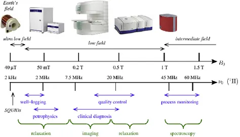
Figure I-2 Summary of the NMR applications on the basis of the static magnetic field strength for permanent magnets (Source: Mitchell et al., 2013)

All of the above techniques have been investigated in food analysis. An overview of the food applications of the liquid state FT-NMR can be found in (Mannina et al., 2012). It presents a review of the NMR methodologies in food quality control, analyzing several aspects as the sample preparation, which is an important step to obtain reproducible spectra, the spectral analysis and the statistical analysis. It also describes some applications to several products like alcoholic beverage, fruits and vegetables, milk and dairy products. An example of food authentication is described in (Parker et al., 2014), in which a bench-top spectrometer has been used for the analysis of olive oil with adulteration of hazelnut oil. A study on the compositional analysis of wine in a full intact bottle has been proposed in (Weekley et al., 2003). In the paper, the capability to detect acetic acid spoilage has been investigated using NMR spectrometry system. An overview of the potential applications of NMR and MRI for compositional and structural analysis, inspection of microbiological, physical and chemical quality, food authentication, on-line monitoring of food processing is presented in (Marcone et al., 2013). A review focused on the

Quality control in hazelnuts processing

7

development of TD-NMR and MRI based sensors for different food applications, can be found in (Kirtil et al., 2017).

Several studies have been carried out on methods and applications of Low Field NMR. A method for Solid Fat Content (SFC) and simultaneous oil and moisture determination has been described in (Todt et al., 2006). Applications on quality control of different food products have been proposed: the evaluation of quality of oranges during storage (Zhang et al., 2012); Analysis of water dynamic states and age-related changes in mozzarella cheese (Gianferri et al., 2007). The interest towards the industrial applications of the TD-NMR is constantly increasing. A study of the perspective of the use of the TD-NMR as in-line industrial sensor can be found in (Colnago et al., 2014). Among the proposed applications in in-line monitoring, Low Field NMR has been employed for the evaluation of the internal browning of whole apples (Chayaprasert and Stroshine, 2005). Moreover, an automated system for oil and water content determination in corn seeds has been proposed in (Wang et al., 2016).

The main applications of the TD-NMR in food quality control are related to the evaluation of the presence of water, moisture, oil, fat, that are well detected by this technique. The quality of the hazelnuts is strictly related to the presence of moisture and fatty acids and then, in this work, Low Field NMR has been taken into account as a suitable technique for the analysis of the hazelnuts quality. In the next chapter, an overview of the NMR methods and the equipment used to carry out the analysis will be depicted.

Chapter II

NMR methods and equipment

II.1 NMR Theory

NMR is based on the magnetic properties of the nuclei of the atoms. The nuclei are characterized by a nuclear spin quantum number (I) that can be equal to or greater than zero, with values multiples of ½. Only the nuclei with a value of I different by zero are NMR-sensitive, while the nuclei with I=0, which are those with atomic mass and atomic number both even, are NMR-silent. The main characteristic of the spinning nuclei is that they possess an angular momentum (P) and charge, and the motion of the charge causes the presence of a magnetic moment (µ). The magnetic moment is proportional to the angular momentum:

𝜇 = 𝛾 ∙ 𝑃 ( 2 )

Where γ is the gyromagnetic ratio, which is constant for each nucleus. When the nuclei are placed in an external static magnetic fields (B0), the

microscopic magnetic moments align themselves relative to the field in a discrete number of orientation, depending on the energy states involved (they depend on the possible spin states). The effect of the static magnetic field on the magnetic moment is to impose a torque that causes a motion of the vector representing the magnetic moment on the surface of a cone around the direction of the field (Fig. II-1).

Figure II-1 Motion of a magnetic moment (μ) of a nucleus in a static magnetic field (B0)

Chapter II

This motion is referred to as Larmor precession and its rate depends on the strength of the applied field and the gyromagnetic ratio of the nucleus.

The rate can be expressed in terms of angular velocity ω0 (rad s-1):

𝜔0= −𝛾 ∙ 𝐵0 ( 3 )

Or frequency f0 (Hz):

𝑓0= − 𝛾

2𝜋𝐵0 ( 4 )

This is named Larmor frequency of the nucleus. For the proton (1_{H) the}

gyromagnetic ratio (γ) is 26.75·107 _{rad T}-1_s-1_{. With a 1 T static magnetic}

field the larmor frequency is 42.25 MHz. In the table II.1, the gyromagnetic ratio, natural abundance and relative sensitivity (to the proton) for the main NMR-sensitive nuclei is shown.

Table II.1 Natural abundance, gyromagnetic ratio and relative sensitivity (to 1H) of some NMR-sensitive nuclei

Nucleus Natural abundance [%] γ [rad T-1_s-1_{] Relative} sensitivity [%] 1_{H 99.98 26.75·10}7 _100.0 13_{C 1.11 6.73·10}7 _1.6 19_{F 100.00 25.18·10}7 _83.3 31_{P 100.00 10.84·10}7 _6.6

The 1_{H nucleus has the highest NMR sensitivity and can be found in most}

materials. For this reason it is the most used in the NMR experiments. At a macroscopic level, the effect of the static magnetic field is a net magnetization vector (M0) on the same direction of the applied field, which is

conventionally considered the z-axis of a Cartesian co-ordinate system (Claridge, 2016). When the nuclei are placed in the field, the magnetization is not instantaneous, but it increases exponentially (eq. 5):

𝑀𝑧(𝑡) = 𝑀0(1 − 𝑒 −𝑡

𝑇1_{) ( 5 )}

The time constant T1 is the longitudinal relaxation time. It is an important

parameter because it can be used to get information about the sample under test during the NMR experiments. Moreover, when a sample is placed in the magnetic field, or after an experiment, it is necessary to wait a period of at least 5T1 to be sure that the magnetization has recovered. This period, on the

basis of the material under test, can be several seconds.

When a material is placed in the static magnetic field and the magnetization process is complete, to obtain a NMR signal it is necessary a radiofrequency (RF) pulse at the Larmor frequency (which is the resonance frequency of the system) that generates an oscillating magnetic field B1 in a plane orthogonal

NMR methods and equipments

11

to the direction of B0. This can be made transmitting the RF pulse to a coil

placed in the static field (Fig. II.2).

Figure II.2 Oscillating magnetic field B1 generated by a RF pulse

transmitted to a coil placed orthogonally in the static magnetic field B0

The effect of B1 is to rotate the magnetization vector, which is along the

z-axis, by an angle θ, called flip angle that can be expressed as:

𝜃 = 𝛾 ∙ 𝑡𝑝∙ 𝐵1 ( 6 )

Where tp is the duration of the RF pulse. At the end of the RF pulse the

magnetization vector returns to the equilibrium and, during this process, it induces a RF voltage in the coil. The maximum amplitude of the voltage is obtained when θ = π/2. When the magnetization vector returns to the equilibrium, the component Mz increases according to eq. (5). This process is

named longitudinal relaxation. At the same time, another independent process occurs, the transverse relaxation, in which the component of the magnetization in the x-y plane decreases to zero. This process is always faster than the longitudinal relaxation. It can be expressed by the eq. (7):

𝑀𝑥𝑦(𝑡) = 𝑀𝑥𝑦𝑒−

𝑡

𝑇2 _{( 7 )}

Where the time constant T2 is the transverse relaxation time. This is,

together with the longitudinal relaxation time (T1), one of the main parameters

used to get quality information about the material under test, in particular in the NMR relaxometry. Conversely, the NMR spectroscopy is based on the frequency domain analysis of the signal induced in the coil at the end of the RF pulse. In the next paragraph a description of the NMR instrument will be depicted.

II.2 NMR equipment

A NMR instrument is composed, regardless of the use as spectrometer or relaxometer, by four main components:

 Magnet;  Probe;

Chapter II

 Transmitter;  Receiver.

II.2.1 Magnet

The magnet is used to generate the static magnetic field B0. The field must

be extremely homogeneous in the volume that contains the sample under test, in order to have the same resonance frequency in the different sections of the sample. The most homogeneous field can be obtained with the superconducting magnets, which are composed by a coil with a wire of superconducting material immersed in liquid helium to maintain the coil at the low temperature needed to guarantee the superconducting property of the wire. These kind of magnets are mainly used in the applications that need high field with the highest homogeneity, like the NMR spectroscopy for chemical analysis. In the low field NMR, permanent magnets are used instead of the more expensive superconductive magnets. They are not able to produce a perfect homogeneous field as required in the NMR spectroscopy, but can be used in the Relaxometry, where several pulse sequences techniques have been developed to limit the effect of the field inhomogeneity and to obtain quality information about the samples under test. Using the permanent magnets allowed a great reduction of the overall cost of the systems and the emergence of the NMR industrial applications.

The main parameter of the magnet is the static magnetic field (B0), which

also determines the resonance frequency of the NMR system (see eq. 4). Other parameters are:

 Field homogeneity (ΔB0/B0);

 Dimension of the field homogeneity area

II.2.2 Probe

The probe is the component that allows transmitting the excitation signals to the samples and receiving the NMR signal in response to the excitation. It is connected both to the transmitter and the receiver and its purpose is to deliver the rotating magnetic field B1 to the sample and to detect the signal at

the end of the excitation RF pulse, during the relaxation time. The main component of the probe is the coil (with inductance L) which is placed inside the magnet in order to obtain a B1 field orthogonal to B0 when the transmitter

sends the RF pulses. The sample under test is arranged in the coil of the probe in order to be subjected both to the static and the rotating fields. The probe also includes two variable capacitors for the frequency tuning (Ctune) and the

impedance matching (Cmatch) (Fig. II.3). The probe circuit is characterized by

three quantities (Teng, 2012):  Resonance frequency;  Impedance at the resonance;

NMR methods and equipments

13

 Q factor.

Figure II-3 Example of probe circuit

The two capacitors are used to adjust the value of the resonance frequency of the circuit to the resonance frequency of the NMR system, and to obtain, at that frequency, an impedance of 50 Ω. The Q factor depends on the resonance frequency and it can be defined by:

𝑄 =𝑓0

∆𝑓 ( 8 )

Where f0 is the resonance frequency and Δf is the bandwidth of the

resonance circuit. In order to increase the probe sensitivity, the probe design is made to obtain the highest value of Q.

II.2.3 Transmitter

The transmitter provides the RF pulses to send to the probe for the sample excitation. It has to be able to generate the RF signals with the requested frequency, phase, amplitude and pulse width. The signals have to be amplified in a power range that depends on the NMR application, and it can be from 10 W to hundreds watt.

Figure II-4 Block diagram of the transmitter

Figure II-4 shows a block diagram of the NMR transmitter. It is composed by three diffeent blocks:

Chapter II

 A timing controller that manages the pulse width and the timing of the pulse sequences;

 A RF signal generator;  A RF power amplifier.

The transmitted RF pulse is a sinusoidal signal at the resonance frequency of the system (f0) with duration tp. It can be expressed in the time domain as:

𝑥(𝑡) = 𝐴 ∏ (𝑡

𝑡_𝑝) 𝑐𝑜𝑠(2𝜋𝑓0) ( 9 )

And in the frequency domain by its fourier transform: 𝑋(𝑓) =𝐴𝑡𝑝

2 [𝑠𝑖𝑛𝑐(𝑓 − 𝑓0)𝑡𝑝+ 𝑠𝑖𝑛𝑐(𝑓 + 𝑓0)𝑡𝑝] ( 10 ) The RF pulses excites the frequencies around the resonance frequency in a bandwidth that depends on the pulse duration tp.

II.2.3 Receiver

The receiver has to be able to detect the weak RF signal from the probe. As previously described (Fig. II-3), the coil of the probe is used both for exciting and for detecting the signal. The excitation pulse is a power signal, so the receiver must be protected when the TX pulses are applied. To do this, the receiver is connected to the probe by means of a device called duplexer and a λ/4 cable (Fig. II.5). The duplexer is made of fast switching diodes. It allows, together with the λ/4 cable, protecting the receiver:

 When the pulse is on, the high power RF is routed to the probe and the receiver is protected by disconnecting it or shorting it to ground;

 When the pulse is off, the receiver is connected to the probe and the transmitter is disconnected.

The received signal is amplified and then a quadrature detection is carried out to obtain a baseband NMR signal from the RF signal.

NMR methods and equipments

15

The following figure shows a block diagram of the receiver:

Figure II-6 Block diagram of the receiver

The received signal has a low-level amplitude that has to be amplified using a low-noise preamplifier that is design to add the lowest possible noise level. In addition, a bandpass filter (BPF) is used in order to filter the noise outside the band of interest before the quadrature detector.

Figure II-7 Block diagram of the quadrature detector The quadrature detector is composed by:

 Local oscillator (LO): it provides a sinusoidal signal with frequency fLO;

 π/2 phase shifter: it provides a sinusoidal signal with a π/2 phase shift respect to the signal generated by the LO;

 Mixer: it multiplies the input signal x(t) and the signal of the LO in the I channel, and the input signal and the phase shifted signal in the Q channel;

 Lowpass filter (LPF).

The signals obtained in the I and Q channel have the frequency: f0 – fLO,

where f0 is the frequency of the input signal x(t).

Chapter II

𝑥(𝑡) = 𝐴𝑐𝑜𝑠(2𝜋𝑓0𝑡) ( 11 )

Where f0 is the Larmor frequency; while the signal generated by the LO and

the π/2 phase shifter can be written, respectively:

𝑥𝐿𝑂(𝑡) = 𝑐𝑜𝑠(2𝜋𝑓𝐿𝑂𝑡) ( 12 )

𝑥𝑆𝐻(𝑡) = −𝑠𝑖𝑛(2𝜋𝑓𝐿𝑂𝑡) ( 13 )

The output of the mixer for the I channel is: 𝑥(𝑡) ∙ 𝑥𝐿𝑂(𝑡) = 𝐴𝑐𝑜𝑠(2𝜋𝑓0𝑡) ∙ 𝑐𝑜𝑠(2𝜋𝑓𝐿𝑂𝑡) =

𝐴

2[𝑐𝑜𝑠2𝜋(𝑓0+ 𝑓𝐿𝑂)𝑡 +

𝑐𝑜𝑠2𝜋(𝑓0− 𝑓𝐿𝑂)𝑡] ( 14 )

While the output for the Q channel is:

𝑥(𝑡) ∙ 𝑥𝑆𝐻(𝑡) = 𝐴𝑐𝑜𝑠(2𝜋𝑓0𝑡) ∙ (−𝑠𝑖𝑛(2𝜋𝑓𝐿𝑂𝑡)) = 𝐴

2[−𝑠𝑖𝑛2𝜋(𝑓0+ 𝑓𝐿𝑂)𝑡 +

𝑠𝑖𝑛2𝜋(𝑓0− 𝑓𝐿𝑂)𝑡] ( 15 )

As can be seen from eq. (14) and eq. (15), at the output of the mixer the signals can be expressed as the sum of two sinusoidal components with frequency f0+fLO and f0-fLO. The component with frequency f0+fLO is filtered using the

LPF, and then only the component with frequency f0-fLO is present at the

output of the quadrature detector.

The frequency of the local oscillator must be equal to the resonance frequency of the system (fLO = f0) in order to have a baseband NMR signal at

the output of the receiver. This is useful because the NMR signals have a narrowband frequency spectrum around the resonance frequency, so the baseband conversion allows simplifying the signal processing.

II.3 NMR methods

Several techniques have been developed to obtain NMR signals in order to extract information like the frequency spectrum, in the case of FT-NMR, or the longitudinal (T1) and transverse (T2) relaxation time, the diffusion

coefficient (D), in the case of TD-NMR. In this work, 1_{H TD-NMR has been}

employed and two pulse sequences have been taken into account:  Single pulse;

 CPMG.

These techniques does not require complex hardware and are relatively fast, so they are suitable for the industrial applications.

NMR methods and equipments

17

II.3.1 Single pulse sequence

Single pulse is the simplest sequence to obtain an NMR signal response. A short and strong RF pulse at the resonance frequency of the system is produced by the transmitter to excite the frequencies in the NMR spectrum; during the RF pulse, the magnetization of the nuclei inside the sample rotates, and the duration of the pulse is chosen to obtain a rotation of the magnetization vector of π/2 rad. At the end of the RF pulse, the nuclei of the sample return to the initial position generating an NMR signal (FID signal).

In order to acquire the FID signal correctly, it is necessary to synchronize the transmitter and the receiver by means of a control signal (Blanking signal).

Figure II-8 Time diagram of the single pulse sequence (Source: Spincore Technologies Inc., 2014)

Figure II-8 shows a time diagram of the single pulse sequence. When the blanking signal becomes active, the RF power amplifier (RFPA) is switched on, and the RF pulse is transmitted to the probe after the blanking delay, that is the time needed to warm-up the RFPA before the RF pulse can start (Fig. II-9). After the pulse time (tp) the blanking signal becomes de-active and the

RFPA is switched off, but the receiver can start to acquire the NMR signal only after the transient time, also named dead time, which is the time needed to switch off the RFPA. After the acquisition time, in which the receiver acquires the FID signal, a new pulse sequence can be started on the same sample only after the repetition delay, which is the time needed to completely recover the magnetization of the sample (eq. 5).

Chapter II

Figure II-9 Blanking signal and RF pulse at the resonance frequency (Source: Spincore Technologies Inc., 2014)

Both the blanking delay and the transient time are related to the RF power amplifier and have to be the shortest possible. In particular, the transient time does not allow acquiring all the FID signal (Fig. II-10).

NMR methods and equipments

19

In a perfectly homogeneous field (ΔB/B0<10-6), the FID signal corresponds

to the transverse relaxation decay (eq.7). In this case, it can be used to calculate the transverse relaxation time (T2) or, alternatively, a Fourier transform can be

carried out to obtain the spectral components of the signal and then the chemical composition of the sample (FT-NMR). Conversely, in presence of a non-homogeneous field, the FID signal decreases faster than the transverse relaxation decay. In this case, the decay is mainly due to the field inhomogeneity, and not to the magnetization of the sample. The exponential decay of the FID signal can be expressed in terms of the time constant T2*

instead of T2, where: 1 𝑇₂∗= 1 𝑇₂+ 𝛾 ∆𝐵₀ 2 ( 16 )

As can be seen from eq. (16), the time constant T2* is inversely proportional

to the static magnetic field variation (ΔB0).

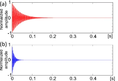
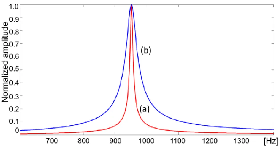
The field inhomogeneity causes a resonance frequency variation in the different sections of the sample. The result is that it is not possible to perform the spectral analysis to determine the molecular structure of the sample. Figure II-11 and Figure II-12 show the effect of the field inhomogeneity in the time-domain and in the frequency-time-domain.

Figure II-11 Effect of inhomogeneity in time domain. (a) Homogeneous field; (b) inhomogeneous field

Chapter II

Figure II-12 Effect of inhomogeneity in frequency domain. (a) Homogeneous field; (b) inhomogeneous field

In the frequency-domain, the faster decay in time corresponds to a broader spectral line, and then a higher frequency resolution that does not allow discriminating the several spectral components related to the molecular composition of the sample. In this case is only possible to perform a quantitative analysis of the liquid part of the sample (that are the molecules containing 1_{H atoms excited at the resonance frequency).}

II.3.1 CPMG sequence

This technique is largely adopted in Low Field NMR because it allows obtaining qualitative information about the sample in presence of field inhomogeneity. In more details, it is used to determine the transversal relaxation time (T2) which is the time constant of the exponential decay of the

NMR signal in presence of a perfect homogeneous field.

The CPMG sequence (Fig. II-13) consists of a π/2 RF pulse (same as the single pulse) followed by a train of π RF pulse (it takes twice the time of the π/2 RF pulse). The distance between the π/2 RF pulse and the first π RF pulse is denoted as τ; the time interval between two π RF pulses is 2τ. The effect of this kind of sequence is to obtain a FID signal after the π/2 RF pulse which has a fast decay due to the field inhomogeneity, and a train of echo signals in the middle of the distance between the π RF pulses; the amplitude of the echo signals gradually decreases after each π RF pulse. The maximum of the amplitude of each echo gives the relaxation curve that can be used to estimate the decay time T2.

The acquisition of the FID signal starts at the time 0. It is generated by the π/2 RF pulse (that is not shown in the figure); after a time τ a π RF pulse is

NMR methods and equipments

21

generated and after a time τ there is the peak of the first echo; an echo is visible each 2τ

Figure II-13 CPMG sequence (first nine echoes)

In the evaluation of the transverse relaxation curve, the odd echoes are usually discarded because the amplitude can be affected by an error due to an incorrect length of the π R pulse, therefore only the even echoes are taken into account.

Figure II-14 Comparison between the transverse relaxation curve obtained with the CPMG (decay with time constant T2) and the decay curve of the FID

signal affected by field inhomogeneity (decay with time constant T2*)

Figure II-14 shows an example of the evaluation of transverse relaxation curve with the CPMG and the comparison between the decay of the curve obtained using the CPMG and the decay of the FID signal that is affected by the field inhomogeneity (see eq.16). As can be seen from the figure:

Chapter II

II.4 The adopted TD-NMR measurement system

The TD-NMR instrument used for the experimental work is composed by three main components:

 NMR console;  Magnet and probe;  Personal computer.

II.4.1 NMR console iSpinNMR™

The NMR console is manufactured by Spincore Technologies Inc. It includes all the electronics to perform the generation and transmission of the excitation pulse sequences as well as the acquisition of the RF signals from the probe. It allows employing a resonance frequency up to 37.5 MHz. The main parameters are:

 Internal RF PA 20 W PEP;

 Internal Arbitrary Waveform Generation;

 DDS for RF output pulse with 14-bit resolution @300 Ms/s;  ADC with 14-bit resolution @75 Ms/s;

 Internal Digital Down Conversion;

 Internal Signal Averaging of Baseband data in multiple acquisitions;  USB 2.0 Interface to transfer data to PC.

A block diagram of the NMR console is depicted in figure II-15. It is composed by three block: (1) The RadioProcessor USB is a digital board that manages the data acquisition, the excitation pulse generation and the timing. In the receiving section, the pre-amplified RF signal from the probe is acquired by a 14-bit resolution ADC and then is demodulated in a digital down converter. In the digital transmitter the RF pulses are generated and converted to analog using a 14-bit resolution DAC. (2) The RF Power Amplification is composed by a RFPA and a low-pass filter. (3) The Small-Signal Pre-amplification is composed by a low-noise 60 dB pre-amplifier and a low-pass filter.

NMR methods and equipments

23

Figure II-15 iSpinNMR™ console block diagram (Source: Spincore Technologies Inc., 2014)

II.4.2 Magnet and probe

These components have been designed for the specific application considering that the probe, placed in the magnet, has to be able to host a whole hazelnut. To this aim, the probe has a cylindrical coil characterized by height and diameter both equal to 25 mm. The permanent magnet has the following characteristics (Figure II-16):

 Air gap: 40 mm;

 Pole face diameter: 150 mm

 Dimension of the uniform magnetic field: 25 mm diameter, 25 mm high;

 Field uniformity: 10-4 _ΔB 0/B0;

 Static magnetic field: 0.513 T at 23.0 °C.

Considering the value of the static magnetic field, the resonance frequency of the system is 21.8 MHz

Chapter II

Figure II-16 Permanent magnet and probe The field homogeneity of the magnet is 10-4 _ΔB

0/B0.This is a typical value

for a commercial permanent magnet. The figure II-17 shows the field variation in function of the position in the x-y plane. Considering a 1_{H probe, a variation}

of 1mT of the static magnetic field causes a variation of the Larmor frequency greater than 40 kHz.

In order to work in the highest homogeneity area, the centre of the coil of the probe must be placed in correspondence of the (0,0) x-y coordinates (Fig. II-17). This point can be found considering the maximum amplitude of the FID signal for a sample at the resonance frequency, achieved moving the probe inside the magnet.

The probe needs to be tuned to the resonance frequency of the system (f0=21.8 MHz) and, in addition, the impedance has to be matched to be

matched to 50 Ω. This has been made by means of a Vector Network Analyzer (Fig. II.18), adjusting the two variable capacitors Ctune and Cmatch (Fig.II-3)

NMR methods and equipments

25

Figure II-17 Field strength as a function of the position in the magnet

Chapter II

II.4.3 Personal computer

The NMR console is connected to a personal computer through an USB 2.0 interface. The complex data of the acquired NMR signal, after a baseband digital down conversion, are stored in an internal RAM memory and then can be transferred to the PC for the automatic processing. A Labview user interface has been implemented to send the setting commands to the NMR console and to carry out the signal processing and the classification algorithm on the received signals.

Figure II-19 Software component diagram of the Labview user interface The Labview user interface makes use of the API functions, provided in a spinapi.dll library by the Spincore Technologies Inc., to send the setting commands to the programmable RadioProcessor board (Fig. II.19).

II.5 Influence parameters in liquid and solid samples

The development of industrial applications with TD-NMR has been possible thanks to the decreasing costs of the electronic components and the use of permanent magnets instead of the more expensive superconducting magnets. However, there are two main disadvantages of using TD-NMR with permanent magnet:

 Field inhomogeneity;

NMR methods and equipments

27

The effects of the field inhomogeneity have been already illustrated in the previous paragraphs.

Permanent magnets have a coefficient of temperature in the order of -1000 ppm/°C, so the static magnetic field, and then the resonance frequency, changes when the temperature changes. In order to limit the resonance frequency variation due to the temperature variation, the magnet has been equipped with a temperature controller and insulated by means of sheets of extruded polystyrene (Fig. II-20).

Figure II-20 Magnet insulated by means of extruded polystyrene sheets

II.5.1 Temperature controller

The temperature controller is composed by:

 2 RTDs PT100 A class placed inside the magnet, near each pole;  2 Peltier Modules, for heating and cooling, placed outside the magnet,

behind each pole;

 1 microcontroller Microchip PIC® 18F4550, implementing the PID control algorithm

Chapter II

The temperature controller allows reducing the temperature variation of the magnet at ± 0.1 °C.

In this way, when the operating temperature is kept at 23.0 ± 0.1 °C the resonance frequency variation is lower than 5 kHz around the nominal value. The following figure shows a block diagram of the temperature controller system:

Figure II-21 Block diagram of the temperature controller

The system is composed by two independent channels, one for each pole of the magnet. The microcontroller acquires the temperature from the two channels on the SPI port. Each temperature sensor is connected to a 22 bit resolution ADC that provides the temperature data on a SPI port connected to the microcontroller (Fig.II-21), which can select the channel by means of a chip select signal. The PID control algorithm, on the basis of the read temperatures, set the value and the direction of the current in the current generators of the two channels, by means, respectively, of a PWM signal and a switch signal. In this way, it is possible to control the heating and cooling level of the peltier cells connected to the current generators.

II.5.2 Other influence parameters

In offline applications, NMR experiments are frequently conducted on liquid samples; solid samples are pre-treated to extract liquid parts, or cut in

NMR methods and equipments

29

pieces for being inserted into the test tube, which is arranged into the probe. In this way, it is possible to use commercial benchtop NMR systems. These kind of systems are used in a laboratory environment, where a strict control of the parameters related to the equipment and the samples is allowed. In particular, the temperature of the sample must be controlled because the NMR signals, e.g. the CPMG signal, are affected by the temperature variations (Carosio et al., 2016). Moreover, some other issues have to be highlighted working with solid samples. This is often the case of inline applications, in which there is no pre-treatment of the material under test. Solid samples are, in many cases, heterogeneous materials with different weight and shape; this causes several effects that do not occur in liquid samples:

 Amplitude variation of the NMR signal and then S/N variation, due to the weight variation of the samples;

 resonance frequency variation due to the different positions of the samples inside the magnet;

 presence of several time constants into the transverse relaxation decay due to heterogeneous samples.

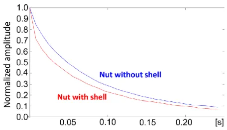
Finally, the physical properties of hazelnuts influence the NMR signals, because of the presence of the shell. Indeed, the hazelnuts are mainly composed by lipids, which are well detected by TD-NMR, while the shell presents some other components, making this product a heterogeneous material. In details, the presence of the shell causes a faster decay of the transverse relaxation signal compared to the unshelled nut (Fig. II-22). Moreover, even considering nuts with the same size, the shape and the weight of the kernel may be very different, affecting the S/N ratio of the NMR signal related to each nut. In particular, being the weight of the kernel closely related to the maximum signal amplitude, the S/N ratio is smaller for lighter nuts (Di Caro et al., 2017).

Chapter II

Chapter III

Hazelnut oil characterization

In order to set-up the instrument for hazelnuts diagnosis

,

preliminarytests were conducted on oil samples extracted from the hazelnuts. In this way, it was possible to concentrate the analysis on the composition of the material without considering some external parameters like humidity or the shape of the sample that can affect the results. This allowed determining the parameters related to the CPMG sequence, and the pre-processing and processing algorithms to carry out the analysis.

III.1 Instrumental parameters

Before starting the analysis on the samples, a test of the NMR instrument has been carried out in order to verify the operation of the equipment (Fig. III-1).

Figure III-1 NMR system test setup

The NMR console provides a TTL output connector where the main internal digital signals are available, this allows checking the timing synchronization of the transmit and the receiving section of the instrument.

In particular, two parameters have been set:  Blanking delay;

 Transient Time (Dead time).

These parameters depend on the system hardware, in particular the RF power amplifier. The former is the time needed to warm-up the amplifier; it

Chapter III

affects the total time of a single NMR experiment because the pulse transmission can start at the end of this delay. The latter is the time needed to ring down the high voltage induced in the coil at the end of the RF pulse. It affects the receiver section because the sample acquisition can start after this time.

The values set are:

 Blanking delay = 3 ms;  Transient time = 16 µs.

The main parameter related to the pulse sequences (both single pulse and CPMG) is the width of the π/2 RF pulse. This is the value that allows rotating the magnetization vector by π/2 respect to the direction of the static magnetic field (eq. 6), and it can be determined using a pulse width finder procedure consisting in calculating the amplitude of the FID signal for several values of the pulse width (tp). The width corresponding to the maximum amplitude of

the FID signal is the width of the π/2 RF pulse (Fig. III-2).

Figure III-2 Pulse width finder procedure

This procedure allows determining the π RF pulse used in the CPMG sequence, which is the pulse width with a null FID signal amplitude. The π RF pulse with is approximately twice as much the π/2 RF pulse width.

Hazelnut oil characterization

33

Applying the pulse width finder procedure in the case of interest the following values have been found:

 π/2 RF pulse width = 8 µs;  π RF pulse width = 16 µs.

III.2 CPMG setup

As described in the chapter II, in order to limit the effect of the field inhomogeneity due to the use of permanent magnets, it is suitable to make use of the CPMG sequence instead of the single pulse

In addition to the width of the π/2 RF pulse and the π RF pulse, the CPMG sequence requires the definition of other parameters (Fig. II-13):

 τ, which determines the distance among the π RF pulse and then the echoes (2τ);

 number of echo to acquire, which determines the acquisition time.  sampling frequency of the received signal;

The time interval between two π RF pulses has been set to 4 ms (τ = 2 ms). This is also the time between the echoes that represent the points of the transverse relaxation decay, so it has been chosen in order to have enough point of the relaxation curve.

For each CPMG sequence, 50 echoes were acquired; the number of echoes is limited by the S/N ratio: when the amplitude of the echo signal is below the noise level, it is impossible to detect the peak.

A sampling frequency of 500 kHz was adopted to have enough points of the CPMG signal for each echo.).

The acquisition time can be calculated from the previous parameters: 𝐶𝑃𝑀𝐺 𝑎𝑐𝑞𝑢𝑖𝑠𝑖𝑡𝑖𝑜𝑛 𝑡𝑖𝑚𝑒 = 𝑁𝑒𝑐ℎ𝑜(𝜋 𝑝𝑢𝑙𝑠𝑒 𝑤𝑖𝑑𝑡ℎ + 2𝜏) + 𝜏 ( 18 )

In this case, the acquisition time is about 200 ms.

III.3 Echo response pre-processing

NMR signals have low amplitude (about 10 µV) and are affected by a high level of noise, due, both to RF interferences and A/D conversion. In the CPMG sequence the amplitude of the echoes decrease at each π RF pulse while the noise level does not change, therefore it is difficult to estimate the amplitude of the last echoes (Fig. III.3).

Chapter III

Figure III-3 Example of acquisition of CPMG signal after 50 ms

Usually, the NMR instruments are able to perform an internal signal averaging over several acquisitions. This allows increasing the S/N ratio of the received signal. In particular:

𝑆

𝑁∝ √𝑁 ( 19 )

Where N is the number of acquisitions of the signal (Fig. III-4).

Figure III-4 Acquired echo signal (45th _{echo) with a single sequence (in}

green) and with an average over 32 sequence (in red)

Considering the acquisition time, and the time interval between two acquisitions on the same sample, which has to be greater than the repetition delay (the time to recover the magnetization at the end of the pulse sequence),

Hazelnut oil characterization

35

the applicability of this procedure is limited to applications that do not require a fast execution time (e.g. laboratory applications).

In this work, in order to better evaluate the amplitude of the echoes that have a lower S/N ratio, avoiding the use of the time consuming multiple acquisitions procedure, a pre-processing of the signal has been performed.

As previously described, each echo peak corresponds to a point of the transverse relaxation decay, and so the relevant information related to the CPMG signal are contained in the acquired samples of the echoes.

Three methods have been evaluated and compared to detect the echo peak amplitudes (Di Caro et al., 2016):

 Mean value of k samples around the peak position;

 Sum of the spectral components of the magnitude of the FFT for the echo signal;

 Maximum of the curve obtained with a polynomial regression on the echo signal.

The echo peaks in the CPMG sequence are located in the middle of the time between two π RF pulses, therefore they are in a known position in the acquired signal.

III.3.1 Mean value

The Mean value method exploits this property to determine the peak position and estimate its value applying a smoothing factor to reduce the effect of noise.

The position (n) of the peak of the i-th echo in the acquired samples is:

𝑛 = 𝑖 ∙ (2𝜏 + 𝜋 𝑝𝑢𝑙𝑠𝑒 𝑤𝑖𝑑𝑡ℎ) ∙ 𝑓𝑠 ( 20 )

Where fs is the sampling frequency of the acquired signal.

The amplitude of the i-th echo peak is calculated as the mean value of the samples in the interval: [n −k

2, n + k 2].

Chapter III

Figure III-5 Mean value method on echo signal with k=12

III.3.2 FFT magnitude

The second method relies on the property that the number of nuclei excited at the resonance frequency is proportional to the area of the FFT magnitude. This is because, for the magnet inhomogeneity, the nuclei in the different sections of the sample are subjected to a different resonance frequency, so their contribution to the FFT magnitude is located in a different frequency respect to the resonance frequency of the system (Fig.II-12). The noise level is calculated and subtracted considering the FFT magnitude outside the frequency range of interest.

Hazelnut oil characterization

37

Figure III-6 FFT magnitude of the echo signal (in red); noise level (in green) The noise level (NL) has been calculated on the basis of the mean value and the standard deviation of the FFT magnitude corresponding to the noise (the green regions in fig. III-6):

𝑁𝐿 = 𝑛𝑜𝑖𝑠𝑒̅̅̅̅̅̅̅ + 𝑠(𝑛𝑜𝑖𝑠𝑒) ( 21 )

III.3.3 Polynomial regression

About the third method, a second order polynomial regression has been applied to the echo signal (Fig. III-7), considering, for each echo, 160 samples around the peak, located at the position according to eq. (20); the echo peak is the maximum of the regression curve (Eq. 22) - (Eq. 24):

𝑦𝑟𝑒𝑔 = 𝑃2𝑥2+ 𝑃1𝑥 + 𝑃0 ( 22 )

∆= 𝑃12− 4𝑃2𝑃0 ( 23 )

𝑚𝑎𝑥 = − ∆

4𝑃2 ( 24 )