and Marine Biogeochemistry
Marco Reale1,2 , Filippo Giorgi1 , Cosimo Solidoro2 , Valeria Di Biagio2 , Fabio Di Sante1,2, Laura Mariotti2, Riccardo Farneti1 , and Gianmaria Sannino3
1Earth System Physics Section, The Abdus Salam International Centre for Theoretical Physics, Trieste, Italy,2National
Institute of Oceanography and Applied Geophysics—OGS, Trieste, Italy,3Climate Modelling Laboratory, Italian National
Agency for New Technologies‐Energy‐Sustainable Economic Development (ENEA), Rome, Italy
Abstract
We introduce a new version of the Earth System Regional Climate model RegCM‐ES and evaluate its performances for thefirst time over the Mediterranean region. The novel aspect of this coupled system is the possibility to simulate the dynamics of the marine ecosystem through abiogeochemical model, BFM (Biogeochemical Flux Model), coupled online with the ocean circulation model MITgcm (MIT general circulation model). The validation of atmosphere and ocean components has shown that the model is able to capture interannual and intermonthly variabilities of the atmospheric heat fluxes and spatial patterns of land surface temperature, precipitation, evaporation, and sea surface temperature with a general improvement compared to previous versions. At the same time, we diagnosed some prominent deficiencies as a warm and dry bias associated in summer with the resolution of the atmospheric module and the tuning of the boundary layer and convective precipitation scheme. On the biogeochemical side, RegCM‐ES shows good skills in reproducing mean values and spatial patterns of net primary production, phosphate, and horizontal/vertical patterns of chlorophyll‐a. Limitations in this case include deficiencies mainly in the simulation of mean values of nitrate and dissolved oxygen in the basin which have been associated with too large vertical mixing throughout the water column, deficiencies in the boundary conditions, and solubility computations. Overall, RegCM‐ES has the potential to become a suitable tool for the analysis of the impacts of climate change on the ocean and marine biogeochemistry in the Mediterranean region and many other domains.
Plain Language Summary
We evaluate the skills of a new version of a regional coupled model in reproducing climate and marine biogeochemistry of the Mediterranean region. Wefind that the model, despite some persistent biases, is able to capture most key aspects of the regional Mediterranean climate and its marine biogeochemistry.1. Introduction
The Mediterranean region (Figures 1a and 1b) is characterized by a complex land‐sea distributions and topo-graphic features affecting heavily both atmospheric and oceanic circulations (Artale et al., 2010; Lionello et al., 2006, 2012; Sevault et al., 2014). The presence of the Mediterranean Sea, which acts as a source of moisture and heat for the atmosphere, along with mountain chains along its coastline, peninsulas, and islands, produces unique atmospheric phenomena such as a well distinct branch of the Northern Hemisphere storm track (Lionello et al., 2016) or the Mistral/Bora winds which blow, respectively, through the Rhone valley into the Gulf of Lions and over the northern Adriatic Sea (Artale et al., 2010). The Mediterranean region lies in a transitional zone between two very different climate regimes, the semidesert regime of northern Africa and the temperate wet regime of central/northern Europe. This makes the Mediterranean a highly sensitive region to global warming, which has in fact been identified as a “hot spot” for climate change (Giorgi, 2006; Giorgi & Lionello, 2008).
The Mediterranean Sea (Figure 1b) can be divided in two subbasins, namely, the western and eastern basins, separated by the Sicily strait. It is connected through the Gibraltar Strait with the Atlantic Ocean and through the Dardanelles Strait with the Black Sea. Its thermohaline circulation is characterized by the pre-sence of three thermohaline cells (Schroeder et al., 2012, and references therein). Thefirst one is an open cell
©2020. The Authors.
This is an open access article under the terms of the Creative Commons Attribution‐NonCommercial‐NoDerivs License, which permits use and distri-bution in any medium, provided the original work is properly cited, the use is non‐commercial and no modifica-tions or adaptamodifica-tions are made.
Key Points:
• A new version of the Earth System Regional Climate Model RegCM‐ES is described and validated in the Mediterranean region • The new development of this
modeling tool is the possibility to simulate the dynamics of marine ecosystems
• The model shows good skills in reproducing net primary production, chlorophyll‐a, and phosphate in the basin
Correspondence to:
M. Reale, [email protected]; [email protected]
Citation:
Reale, M., Giorgi, F., Solidoro, C., Di Biagio, V., Di Sante, F., Mariotti, L., et al. (2020). The regional Earth system Model RegCM‐ES: Evaluation of the Mediterranean climate and marine biogeochemistry. Journal of Advances
in Modeling Earth Systems, 12, e2019MS001812. https://doi.org/ 10.1029/2019MS001812
Received 10 JUL 2019 Accepted 10 JUN 2020
associated with inflow of relatively cold and fresh water at the Gibraltar strait which moves eastwards along the northern African coastlines, following a cyclonic circulation and undergoing a progressive increase of salinity due to evaporation. In fact, the Mediterranean Sea is mainly an evaporative basin where evaporation exceeds precipitation and river input. This modified (through evaporation) subtropical near‐surface Atlantic water undergoes a further increase in salinity and eventually sinks in the area of the Rhodes Gyre and Levantine basin (Schroeder et al., 2012, and references therein) giving rise to an intermediate current located roughly between 200–500 m (the Levantine Intermediate Water) flowing westwards and eventually outflowing into the Atlantic Ocean at the Gibraltar Strait (Schroeder et al., 2012, and references inside). The Levantine Intermediate Water has been recognized as an important driver of the two other closed thermohaline cells. One is located in the western basin and is associated with deep water formation processes taking place in the Gulf of Lions (Schroeder et al., 2012, 2016). The other is located in the eastern basin and is associated with deep water formation processes taking place mainly in the southern Adriatic (Mantziafou & Lascaratos, 2004, 2008). Model studies and observational evidences have challenged the idea of stationarity in the behavior of these cells (Beuvier et al., 2010; Roether et al., 2007). In particular, the appearance of the Eastern Mediterranean Transient (Roether et al., 2007), with a shift of deep water formations processes from the southern Adriatic to the Aegean Sea, has suggested the existence of multiple equilibria in the thermohaline cell of the Eastern Mediterranean Sea (Amitai et al., 2016; Ashkenazy et al., 2012; Reale et al., 2017).
From a biogeochemical point of view the Mediterranean Sea is known as an oligotrophic basin (ultraoligo-trophic in its eastern part), characterized by a low‐level of productivity compared to the global ocean (Lazzari et al., 2012) and a clear west‐east trophic gradient in productivity (D'Ortenzio & Ribera d'Alcala, 2009; Lazzari et al., 2012). This results from the superposition of a biological pump, the estuarine inverse circulation and the location of sources (rivers, atmospheric deposition, convective, and upwelling regions) of nutrients, namely, nitrogen (N) and phosphorus (P) (Crise et al., 1999; Crispi et al., 2001). Subtropical near‐surface Atlantic Water is relatively poor in nutrients and the aforementioned sources are not able to enrich it as it progresses into the basin. Thus, it leaves the area without changing significantly the oligotrophy of the basin (Lazzari et al., 2016). The only exceptions to this are the areas of the basin (such as Gulf of Lions, Strait of Sicily, Algerian coastlines, southern Adriatic, Ionian Sea, Aegean Sea, and Rhodes Gyre) where strong vertical mixing and upwelling phenomena associated with air‐sea interactions and wind stress field enriches the surface with nitrate (NO3) and phosphate (PO4) favoring phytoplankton
growth (i.e., blooms) mainly in the late winter‐early spring (D'Ortenzio & Ribera d'Alcala, 2009). A proxy for these blooms in the marine environment is the chlorophyll‐a concentration in the upper layer of the basin. Satellite and modeling studies (D'Ortenzio & Ribera d'Alcala, 2009; Lazzari et al., 2012) have shown that in the open Mediterranean Sea, chlorophyll‐a rarely exceeds 2–3 mg/m3
and is characterized by rela-tively large values in specific areas where it is strongly linked to physical forcing, such as wind stress and heat fluxes, and near the coast close to river mouths (D'Ortenzio & Ribera d'Alcala, 2009; Lazzari et al., 2012).
Figure 1. (a) RegCM4 domain and topography (in m) over the Mediterranean region. (b) Ocean model bathymetry (in m) and the river locations defined in the model (cyan squares).
A realistic representation of the complex air‐sea interactions that shape both climate and biogeochemical dynamics of the Mediterranean marine ecosystems requires the use of tools capable of representing thefine scales of these processes, such as coupled Atmosphere‐Ocean Regional Climate Models (AORCMs, e.g., Giorgi & Gao, 2018). In an AORCM different models simulate the dynamics of specific components of the climate system, such as atmosphere, ocean, lake, soil, river, and marine ecosystems. A coupler manages the integration of the models and the exchanges of information across different subcomponents. Over the last years, various high resolution AORCMs have been developed and tested over the Mediterranean region (Artale et al., 2010; Drobinski et al., 2012; Herrmann et al., 2011; Sevault et al., 2014; Somot et al., 2008; Turuncoglu & Sannino, 2016). For example, the Protheus System (Artale et al., 2010), an AORCM composed by the atmospheric model RegCM3 (Pal et al., 2007) and the ocean model MITgcm (Marshall, Adcroft, et al., 1997; Marshall, Hill, et al., 1997) coupled through the OASIS system, has been shown to realistically reproduce the interannual and seasonal variability of sea surface temperature (SST), wind fields and air‐sea interactions over the basin. The Morce system (Drobinski et al., 2012), using WRF for the atmosphere (Skamarock et al., 2008) and NEMO for the ocean (Madec, 2008), includes also a module for land vegetation dynamics (ORCHIDEE, Krinner et al., 2005), atmospheric chemistry (CHIMERE, Bessagnet et al., 2008), and two biogeochemical modules (PISCES and Eco3; Aumont et al., 2003; Baklouti, Diaz, et al., 2006; Baklouti, Faure, et al., 2006). Morce has been employed to analyze the Mediterranean seawater budget, extreme events (intense winds and precipitation) and the impact of vegetation evolution on the water cycle of the Mediterranean region. Sevault et al. (2014) described the performance of the fully coupled system CNRM‐RCSM4 which includes a module for the atmosphere (ALADIN, Herrmann et al., 2011), land surface (ISBA, Noilhan & Mahfouf, 1996; Noilhan & Planton, 1989), rivers (TRIP model, Oki & Sud, 1998), and ocean (NEMOMED8; Madec, 2008) managed by the OASIS coupler system. This model has shown high skills in reproducing the interannual and decadal variability of air‐sea fluxes, river runoff, SST, sea surface salinity (SSS), and the Eastern Mediterranean Transient (Sevault et al., 2014). Finally Turuncoglu and Sannino (2016) developed RegESM, an AORCM composed by RegCM4 for the atmosphere (Giorgi et al., 2012), BATS as land surface scheme (Dickinson et al., 1993), ROMS for the ocean (Haidvogel et al., 2008; Shchepetkin & McWilliams, 2005) and the ESMF coupler (Collins et al., 2005; Hill, DeLuca, Balaji, Suarez, & da Silva, 2004; Hill, De Luca, Balaji, Suarez, da Silva, et al., 2004).
This study aims at introducing a new version of the Earth System Regional Climate Model RegCM‐ES (Sitz et al., 2017) as applied to the Mediterranean basin. RegCM‐ES includes RegCM4 (Regional Climate Model; Giorgi et al., 2012) as atmospheric module, CLM4.5 (Community Land Model, Oleson et al., 2010) as land surface scheme, MITgcm (MIT general circulation model, Marshall, Adcroft, et al., 1997; Marshall, Hill, et al., 1997) as ocean component, and a river routing scheme, HD (Hydrological Discharge Model, Hagemann & Dumenil, 1998, 2001). Earlier versions of RegCM‐ES were tested over different CORDEX regions (Giorgi et al., 2009) such as the South Atlantic (Barreiro et al., 2018), Central America, South Asia (Di Sante et al., 2019), and in the tropical band configuration (Sitz et al., 2017). The new version of RegCM‐ES presented in this study, including an updated version of RegCM4, offers the possibility to simu-late the dynamics of marine ecosystems through a biogeochemical module, BFM (Biogeochemical Flux Model, Vichi et al., 2015), coupled online to the ocean model MITgcm (Figure 2a). Here we assess this model version against available observations for a suite of both physical and biogeochemical variables using a mul-tiyear simulation driven at the lateral boundaries by ERA‐interim reanalysis (Dee et al., 2011).
The paper is organized as follows: in section 2 we introduce the new version of RegCM‐ES and describe its setup for the Mediterranean region. In section 3 we evaluate its performance in the Mediterranean region against observational and modeled data sets. Conclusions are summarized in section 4.
2. The Regional Earth System Model RegCM‐ES
The modeling framework of RegCM‐ES (Figure 2a) includes as atmospheric component RegCM4 (Giorgi et al., 2012), the CLM4.5 as land surface scheme (Oleson et al., 2010), the MITgcm as ocean component (Marshall, Adcroft, et al., 1997; Marshall, Hill, et al., 1997), HD as river routing model (Hagemann & Dumenil, 1998, 2001), and the BFM model (Vichi et al., 2015) for the marine biogeochemistry. Table 1 sum-marizes the setup and main parameters for the numerical experiments presented in this work.
2.1. Model Structure and Experimental Setup
The RegCM4 (Giorgi et al., 2012) system is based on the primitive equations mesoscale model MM5 devel-oped at the National Centre for Atmospheric Research (NCAR) and Pennsylvania State University (Grell et al., 1994). It is a compressible and sigma‐p vertical coordinate model which uses an Arakawa B‐grid to hor-izontally stagger wind and thermodynamical variables (Giorgi et al., 2012). We employ here the Version 4.6.1 which has been developed on the basis of versions 4.4.5/4.5 used and validated in Giorgi et al. (2012) and Sitz et al. (2017). The domain of the atmospheric module covers approximately the Med‐Cordex domain (Ruti et al., 2014), which encompasses the entire Mediterranean Sea basin (Figure 1a). The atmospheric grid has a horizontal resolution of 30 km on a Lambert conformal projection, with the domain centered at 19°E and 43°N, and 23 vertical sigma levels. The model is used in its hydrostatic configuration. Initial and lateral boundary conditions for wind, sea level pressure, air temperature, and specific humidity at 6‐hourly fre-quency are derived from the ERA‐Interim reanalysis at 0.75° resolution (Dee et al., 2011). Lateral boundary conditions are implemented with a buffer zone width of 16 grid points, using an exponential relaxation pro-cedure (Giorgi et al., 1993). The model uses the Zeng Ocean Air‐Sea scheme (Zeng et al., 1998) to parame-trize air‐sea exchanges. We selected the following parameterization schemes of RegCM4: the Holtslag scheme for planetary boundary layer representation (Holtslag et al., 1990), the Subex scheme for large scale precipitation (Subgrid Explicit Moisture Scheme, Pal et al., 2000), the Tiedtke parametrization for cumulus convection (Tiedtke, 1989), and the CCM3 radiative transfer scheme (Kiehl et al., 1996) as modified by Giorgi and Mearns (1999) for radiative transfer calculations. For the representation of land surface processes RegCM4 uses CLM 4.5 (Oleson et al., 2010), a state‐of‐the‐art land surface model which can be employed to describe dynamic vegetation processes, carbon and nitrogen cycle along with hydrology (Oleson et al., 2010). Although CLM4.5 allows the user to run the model using either a prescribed phenology which evolves in time according to IPCC guidelines or a dynamical vegetation, due to the relative short length of the simulation we prefer to use a prescribed phenology based on MODIS data (Lawrence & Chase, 2007). In our experiments we do not consider the contribution of aerosol and gas chemistry. The timestep of RegCM is equal to 30 s.
The MITgcm (Marshall, Adcroft, et al., 1997; Marshall, Hill, et al., 1997) is a primitive equation ocean model based on the Boussinesq approximation of the Navier‐Stokes equations. It can be run on different types of grids (e.g., cartesian, spherical, and cylindrical) with a z‐vertical level discretization. It uses a finite element volume approach and partial cells to treat complex geometries, in either hydrostatic or nonhydrostatic con-figurations. The resulting horizontal and vertical velocities components are staggered on a Arakawa C and Lorenz grid. The code version employed is the 65 s which has been modified with respect to Sitz et al. (2017) Figure 2. (a) Scheme of RegCM‐ES: RegCM.4.6.1 is the regional climate model which includes CLM 4.5 as land surface scheme; MITgcm is the ocean general circulation model which includes, through the BFMcoupler package, the coupling with the BFM model for the marine biogeochemistry; HD is the river discharge model; ESMF is the driver, which manages the time integration of each module and the interpolations and exchanges of forcingfields. (b) Simulated values by RegCM‐ES of downward shortwave radiation (blue, in W/m2) and PAR (green, inμE m−2s−1) at the top of the water column at the center of the Mediterranean Sea in a numerical test of approximately 7 days.
to include some additional subroutines and a new package called BFMcoupler to allow the coupling between MITgcm and BFM (Cossarini et al., 2016). The domain of the ocean model covers approximately the Mediterranean Sea plus a (closed) buffer zone in the Atlantic Ocean (both shown in Figure 1b). The Black Sea and Marmara Sea are not included in the domain. The domain has been discretized using a curvilinear grid and has a horizontal resolution of 1/12° in both zonal and meridional directions, which translates approximately 9 km in the horizontal, and the model can be considered eddy permitting, being the Rossby radius approximately 10 km in the basin. In the vertical the model has 75 unevenly distributed levels. The parametrizations used in our simulations are similar to those used in the MedMIT12 experiment described in Harzallah et al. (2016), Llasses et al. (2016), Reale et al. (2017), and Cusinato et al. (2018). The model employs a linear free surface for the upper boundary of the domain, the GGL scheme for vertical mixing and the third order DST (direct space‐time) scheme with flux limiter for the advection of both physical and biogeochemical tracers. The timestep of the model is 120 s. As initial conditions, velocities are null across the domain, whereas initial temperature and salinity are given by the mean 3‐D temperature and salinity from the Rixen data set for year 1994 (Rixen et al., 2005). The exchanges of water at the Gibraltar Strait are achieved by relaxing (with a relaxation time equal to 2 days) the 3‐D temperature and salinity fields in the Atlantic buffer zone to an updated version of Levitus monthly climatology (Boyer et al., 2013) as described in Reale et al. (2017) and Cusinato et al. (2018). As Table 1
RegCM‐ES Setups and Parameters Used in This Study Atmosphere
Model RegCM.4.6.1
Land surface scheme CLM 4.5
Configuration Hydrostatic
Horizontal resolution 30 km
Vertical resolution 23 sigma p levels
Time step 30 s
Convective scheme over land/ocean Tiedtke/Tiedtke Planetary boundary layer Holtslag Resolvable scale precipitation scheme Subex
Initial conditions ERA‐Interim 0.75°
Lateral boundary conditions ERA‐Interim 0.75°
Ocean/biogeochemistry
Model(s) MITgcm/BFM
Configuration Hydrostatic
Horizontal resolution 1/12°
Vertical resolution 75 z levels
Time step 120 s (for the physics)/600 s (for the biogeochemistry)
Vertical mixing GGL90
Advective scheme for tracers (physical and biogeochemical)
Third‐order direct space‐time scheme with flux limiter
Initial conditions Rixen climatology for temperature and salinity/MEDAR‐MEDATLAS data set for dissolved oxygen, NO3, PO4and silicate/BFM standard values for all the other biogeochemical variables
Lateral boundary conditions Levitus climatology for temperature and salinity/World Ocean Atlas 2013 for dissolved oxygen, phosphate, nitrate, and silicate/Huertas et al. (2009) and Dafner et al. (2001) for alkalinity and dissolved inorganic carbon/equal to initial conditions for all the other biogeochemical variables/atmospheric deposition from Ribera d'Alcala et al. (2003)/river biogeochemical input from Ludwig et al. (2009)
Hydrology
Model HD 0.5° together with MedCordex Protocol (only for Nile River) /Kourafalou and Barbopoulos (2003) (only for Dardanelles Strait)
Driver
Library ESMF/NUOC
Frequency of coupling 1 hr (ocean/atmosphere), 1 day (atmosphere/river and river/ocean) Period of the simulation 1994–2006
additional lateral boundary conditions the model adopts the no‐slip conditions at lateral boundaries and at the bottom. Since the ocean domain is closed, its volume balance is controlled by evaporation (E), precipita-tion (P), and river runoff (R). Our model configuraprecipita-tion computes at every time step the integral over the basin (excluding the buffer zone in the Atlantic) of the E‐P‐R flux. This value is subtracted as a freshwater flux in the Atlantic Buffer zone, forcing the conservation of volume in the domain. No further surface fluxes are considered in the Atlantic buffer zone, where the 3‐D relaxation to temperature and salinity is applied. The BFM (Vichi et al., 2015) is able to simulate the dynamics of plankton (both phyto and zooplankton), bac-teria, oxygen, carbon, nitrogen, phosphorus, silica cycles within the marine ecosystem and among trophic levels. It can also be employed to simulate the dynamics of the carbonate system and exchanges of O2/CO2between atmosphere and ocean. BFM has been extensively applied to the study of the dynamics
of NO3, PO4, Chlorophyll‐a and Net primary production (Lazzari et al., 2012, 2016) in the Mediterranean
Sea, marine carbon sequestration (Canu et al., 2015), spatial and temporal variability of alkalinity (Cossarini et al., 2015), extreme events in marine biogeochemistry (Di Biagio, 2017), impacts of climate change on the biogeochemical dynamics of marine ecosystems (Lamon et al., 2014; Lazzari et al., 2014) as well as for biogeochemical projections in the Mediterranean Copernicus system (Teruzzi et al., 2016). The configuration of the BFM adopted in this work is the Version 2. Initial and lateral boundary conditions for the biogeochemical variables at the Gibraltar Strait follow the approach of Di Biagio et al. (2019) for the MedMIT12‐BFM system. Initial conditions for dissolved oxygen, nitrate, phosphate and silicate are based on the vertical profiles discussed by Crise et al. (2003) and Manca et al. (2004) (taken from the MEDAR/MEDATLAS data set, 2002). For the other biogeochemical variables (e.g., plankton groups), the initial conditions values are set to the standard BFM values in the top 200 m due to the lack of data. Lateral boundary conditions for alkalinity and dissolved inorganic carbon are derived from the data profiles published by Huertas et al. (2009) and Dafner et al. (2001) while for dissolved oxygen, phosphate, nitrate and silicate they are obtained from the World Ocean Atlas 2013 data set (https://www.nodc.noaa.gov/OC5/ woa13/). Due to the lack of data the other biogeochemical variables are set equal to the initial conditions. The profiles adopted for the biogeochemical boundary conditions at the Gibraltar Strait do not consider a seasonal cycle or a time evolution. This is because in most cases these profiles and timeseries are not avail-able or are characterized by too large uncertainties in their vertical profiles and magnitude or by the absence of significant differences at the seasonal scale. Future experiments will use more advanced global biogeo-chemical reanalysis to force the model at the Gibraltar strait. Additional lateral boundary conditions are con-sidered to parametrize the ATI of nutrients, alkalinity, dissolved organic carbon and silicate through atmospheric deposition (only for nitrate and phosphate) and river input (for all of them). Following Di Biagio et al. (2019), the atmospheric deposition of phosphate and nitrate is parametrized as a molar mass rate entering in the surface cells of the ocean model and is set equal to the values tabulated in Ribera d'Alcalà et al. (2003). For the Mediterranean river load, original annual river load data for the Mediterranean basin (including also the Dardanelles Straits) are available since 1960 as tabulated by Ludwig et al. (2009) and are converted in molar mass rates entering the surface cells in correspondence of the river mouth, modulated according to a seasonal cycle, as described in Di Biagio et al. (2019).
Finally, to simulate the freshwaterfluxes at the land surface we use HD (Hagemann & Dumenil, 1998, 2001) which computes the discharge on afixed 0.5 resolution global grid with a daily time step. The total outflow from a grid box is given by the sum of three different types offlows: overland, base, and river flow (Sein et al., 2015; Sitz et al., 2017). The overlandflow uses surface runoff as input and represents the fast flow com-ponent within a grid box, the baseflow uses the subsurface runoff and represents the slow component, while the riverflow represents the inflow in a grid box from the nearby grid boxes (Sein et al., 2015). The HD ver-sion adopted here is the same adopted in Sitz et al. (2017). The river discharge values for the Mediterranean rivers are computed online by HD except for the Nile river which are based on the Med‐Cordex protocol values. As Black Sea and Marmara Sea are not included in our domain, the inflow of water from the Black Sea is parametrized as river with discharge values based on the monthly climatological net inflow rates available in Kourafalou and Barbopoulos (2003).
Given that observed biogeochemical data for model validation are available only since the mid‐1990s (Crise et al., 2003; Colella et al., 2016; Lazzari et al., 2012, 2016; Manca et al., 2004; MEDAR, 2002; Teruzzi et al., 2016), the model is integrated for the period 1994–2006.
Numerical experiments presented here do not consider a spin‐up procedure, since performing a spin‐up for the biogeochemical part of the model on a highly resolved computational grid is extremely challenging (Sein et al., 2015) and because, as observed in previous studies (e.g., Sitz et al., 2017), regional ocean models might benefit from being in a state as close as possible to observations and the use of lateral boundary conditions in a small closed domain as the Mediterranean region imposes a control on the numerical solutions (Sitz et al., 2017). Figure 3 shows the mean annual temperature and salinity, the mean annual concentration of phosphate, nitrate, chlorophyll‐a, dissolved oxygen and the net primary production at 20, 150, 250, and 500 m depths. The initial drifts displayed by all the time series during the first 6 years of simulation (1994–1999) are reduced in the following years. More specifically after 2000 and at the surface, drifts for Figure 3. Mean annual temperature and salinity; the mean annual concentration of phosphate, nitrate, chlorophyll‐a, dissolved oxygen, and the net primary production at 20 (blue), 150 (red), 250 (black), and 500 m (fuchsia).
temperature and salinity are not significant, for phosphate and nitrate are reduced of an order of magnitude and in the case of net primary production, chlorophyll‐a and dissolved oxygen are reduced by a factor of 5. In the interior drifts are not significant in all the variables, except the oxygen below 150 m. In this case there is a steady increase in concentration. This behavior is most probably a consequence of the relative short length of the simulation which does not allow a balance between respiration processes and reoxygenation of the bot-tom layers through vertical mixing. Net primary production shows relatively small negative values below 200 m. The BFM model computes the net primary production as a difference between phytoplankton gross primary production and phytoplankton respiration/excretion of photosynthesized carbon in conditions of nutrient shortage (Vichi et al., 2015). Due to the attenuation of light with depth below 200 m respiration pro-cesses prevail over photosynthesis and this explains the negative sign observed in Figure 3.
We thus set the starting point of our quantitative analysis at year 2000, and we considered only thefirst top 150 m for the biogeochemistry evaluation. Only for SST we used the entire period 1994–2006.
2.2. Coupling
The coupling procedure in RegCM‐ES is the same adopted in Sitz et al. (2017). It relies on a driver which manages the integration of each component and the exchanges offields among them (Figure 2a). The driver of the system is based on ESMF/NUOC libraries and has been extensively described in previous studies (Sitz et al., 2017; Turuncoglu & Sannino, 2016; Turuncoglu et al., 2013). In this configuration it has been modified to allow the inclusion of BFM libraries in the coupling system. Through the driver (Figure 2a) the atmo-sphere receives every hour the SST from the ocean module. The latter receives, with the same frequency, the following atmospheric variables: total heatfluxes, evaporation minus precipitation, zonal and meridio-nal components of wind speed, atmospheric pressure, and downward shortwave radiation. Since all these quantities are discretized on different grids, the driver remaps them on the grid of the receiving model. The coupling between the ocean model and the marine biogeochemical module occurs everyfive ocean time steps (thus every 600 s) following a processor splitting scheme described in Cossarini et al. (2016). As shown in Figure 2a the variation in a certain time interval of a generic biogeochemical variable (dC), can be consid-ered as the sum of two processes: advection/diffusion processes (dCphys) and biogeochemical reactions
(dCbiol). dCphysis computed by the MITgcm through its tracers package (PTRACERS), whereas dCbiolis
cal-culated by the BFM and transferred back to the MITgcm through the BFMcoupler package included in the ocean model code. The two values are then added by the MITgcm through the GCHEM package providing the overall dC. Several processes occurring in the marine environment are influenced by sea temperature and light. Sea temperature regulates all the physiological processes in the water column whereas light is the primary source of energy in the photosynthesis processes operated by phytoplankton. Only a portion (the so‐called Photosynthetic Available Radiation or PAR) of the incoming light is used for phytoplankton growth. In BFM, light attenuates with depth according to a Lambert‐Beer law with an attenuation coefficient given by water turbidity and suspended/dissolved water components (Vichi et al., 2015). The downward shortwave radiation is used by the ocean model to compute the PAR (Figure 2b) which is transferred together with the temperature (the effect of salinity on the biogeochemistry are here neglected) to the bio-geochemical module through the BFMcoupler.
The river discharge model receives from the land surface module CLM the surface and subsurface runoff once a day. These are then interpolated on the HD 0.5 × 0.5 grid, where the river catchment is defined. The hydrological model is used then to route the water toward the oceanic mouths where the coupler (Figure 1b) uniformly distributes the runoff as a freshwaterflux over the ocean surface and is summed to the precipitation contribution. The runoff does not have a salt concentration value associated and affects the salinity through dilution. A radius of 20 km has been chosen to calculate the ocean grid points where the runoff is interpolated.
3. Results
3.1. Atmosphere
In order to validate RegCM4 and to assess the effect of the model coupling, runs with (COUPL) and without (ATM) ocean coupling, where SST are obtained from the ERA‐Interim reanalysis at 0.75° resolution (Dee et al., 2011) are compared. More specifically we compared patterns and mean values of simulated surface
air temperature and precipitation throughout the model domain with two observational data sets: 0.25° CRU (Climate Research Unit, New et al., 2000) and GPCP (Global Precipitation Climatology Project, Huffman et al., 2001).
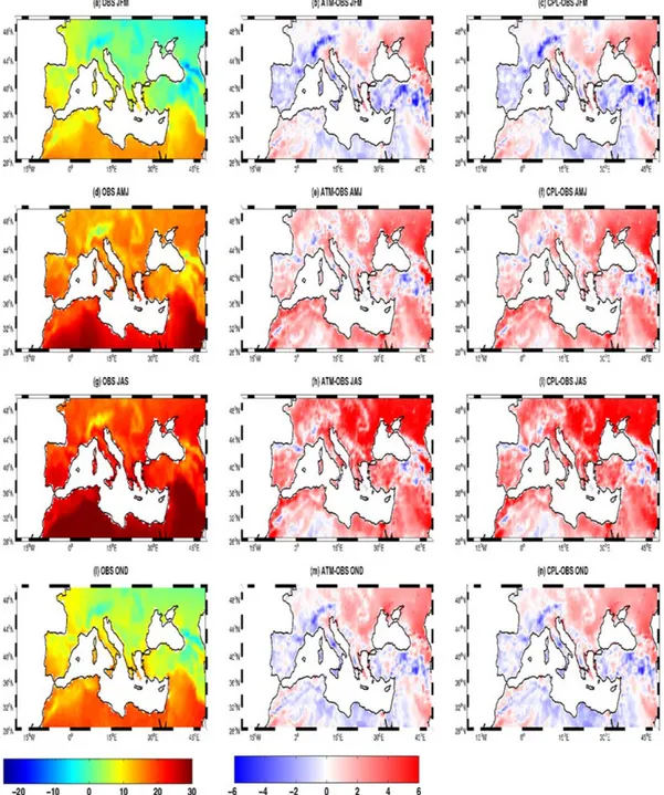
Figure 4 shows the seasonal climatology of land surface temperature from the CRU observations and the corresponding biases for ATM and CPL in January‐February‐March (JFM), April‐May‐June (AMJ), July‐ August‐September (JAS) and October‐November‐December (OND). RegCM4 reproduces the observed surface spatial patterns in both simulations in winter and fall, where biases are within ±2°C. The overall bias in the region shown in Figure 4 is 0.07°C in winter and 0.27°C in fall. However, a significant negative bias is Figure 4. Seasonal climatology of observed (CRU) land surface temperature (first column, a, d, g, j) in JFM (first row), AMJ (second row), JAS (third row), and OND (fourth row) at 2 m and the differences of model simulations RegCM4 (ATM, second column) and RegCM‐ES (CPL, third column) in the period 1994–2006. Units are °C.
still present over the mountains chains (Alps, Dinaric Alps, Pyrenees, Anatolian peninsula), at least partially associated with the prevalence of valley observing stations and topography resolution (Giorgi et al., 2012; Sein et al., 2015; Turuncoglu & Sannino, 2016). In this regard, the RegCM4 configuration used here significantly reduces the magnitude of cold biases over the Iberian peninsula, southern Italy, Greece, and northern Africa in both JFM and OND (not shown), as compared to the RegCM3 system adopted by Artale et al. (2010) and (in absolute value) the cold biases of 2°C reproduced in the region in the RegCM.4.4.5. An average warm bias of 2.2°C is found in summer, with local peaks exceeding 4°C over large portion of the region, mostly associated with a negative precipitation bias (Figure 5) as described in other studies (Turuncoglu & Sannino, 2016; Turuncoglu et al., 2013). The annual‐mean bias over the region with respect to CRU data set is equal to 1°C for both ATM and CPL simulations.
Figure 5 shows the seasonal climatology of GPCP precipitation (first column) and associated biases in the ATM (second column) and CPL (third column) simulations. Simulated spatial patterns and magnitude of precipitation are consistent with observations, despite the fact that the model tends to overestimate precipi-tation over the high topography (as observed in Giorgi et al., 2012), especially in winter and fall and over the Mediterranean Sea in winter. This bias over land, however, may be artificially amplified by the lack of an undercatch gauge correction in the observational data. On the other hand the model tends to underestimate precipitation in summer, as noted in previous studies (Fantini et al., 2018), over Eastern Europe, the Adriatic Sea and over land in fall. Furthermore, an increase/decrease of the precipitation biases over the Aegean Sea and Rhodes gyre area/southern East Mediterranean Basin is observed in the CPL simulation during the fall. A comparison of ATM and CPL shows that the effect of coupling on precipitation is not large, but the cou-pling slightly improves the representation of precipitation in winter and fall over the southern East Mediterranean Sea. At the annual scale the average bias over the region between both simulations and GCPC data is−0.26 mm day−1. However, the magnitude of this bias could be underestimated because of the aforementioned lack of an undercatch gauge correction in the observational data.
We identified the origin of the warm and dry biases found in all simulations in the Holtslag scheme adopted to parametrize the boundary layer and in the Tiedtke scheme used to parametrize the convection. The for-mer tends to overestimate the vertical transport of heat in stable and dry conditions (Turuncoglu et al., 2013) as in summer and spring and to underestimate the cloud cover giving rise to higher temperatures at the sur-face. The latter depends on the two parameters dealing with the entrainment rate for convection over land and over the ocean and the conversion coefficient for the cloud cover. These values are, in our configuration, probably too low to proper reproduce convective precipitation over the region in both summer and spring when these phenomena are more frequent (Miglietta et al., 2017).
Figures 6a–6e show the temporal evolution of the four different components of the heat budget (net short-wave, net longshort-wave, latent and sensible heatfluxes) and precipitation compared with two observational data set: OAflux (Ocean‐Atmosphere flux, Yu et al., 2008) and NOCS (National Oceanography Centre Southampton Version 2.0, Berry & Kent, 2011). Both data sets have been averaged over the Mediterranean Sea. The spread of the observational curves represents the uncertainty associated with the two observational data sets. Table 2 shows the mean values of the four components of the heat budget com-puted for the period 1994–2006. We limited the analysis of the heat fluxes over the Mediterranean Sea as they represent the forcing of the ocean model.
Both the ATM and CPL simulations show a similar mean net shortwaveflux of 206 W/m2over the period 1994–2006, overestimating observations by about 30 W/m2when compared with OA. This value has been found to be in the range of NOCS data set ([164; 210], Table 2). This value is also comparable with that found in RegESM (Turuncoglu & Sannino, 2016), and about 10 W/m2larger than what found in CNRM‐RCSM4 (196 W/m2, Sevault et al., 2014). This overestimation is particularly pronounced in spring and summer (more than 40 W/m2, not shown), and it is maximum along the northern African coastlines and over the northern Western Mediterranean, Adriatic and Aegean Sea (not shown; Sevault et al., 2014; Turuncoglu & Sannino, 2016). The observed overestimation of the shortwave has been associated mainly with the under-estimation of cloud cover over the region (not shown) in spring and summer derived from the use of the Holtslag scheme for the boundary layer and secondarily, with the use of the Era‐interim lateral boundary conditions for the atmosphere, given that also the reanalysis product is characterized by a general overesti-mation of net shortwave radiation (Turuncoglu & Sannino, 2016). Both the ATM and CPL (Figure 6b) have similar values of net longwave radiation (−77 W/m2
), which is a bit larger than the value from the OA data set (−70 W/m2) and in good agreement with the net longwave estimate of Sanchez‐Gomez et al. (2011) based on ISCCP2 data set (−76 ± 4 W/m2
). The values found show a slight improvement with respect to those found in RegESM and CNRM‐RCSM4 which in both cases fall in the interval [−81; −82] W/m2(Sevault et al., 2014; Turuncoglu & Sannino, 2016). The mean latent heat loss (Figure 6c) is−117.22 W/m2for ATM and−116.54 W/m2for CPL, that is,−30 W/m2larger than the values from OA ([−96; −78] W/m2) and in the range of observations of NOCS ([−122; −44] W/m2). Note that the ATM is in better agreement with observations than that found in RegESM (−121 W/m2, Turuncoglu & Sannino, 2016) and the ALADIN standalone simulation used in CNRM‐RCSM4 (−120 W/m2, Sevault et al., 2014). On the other hand the value found in CPL is slightly higher than that computed in RegESM (−110 W/m2
& Sannino, 2016) and CNRM‐RCSM4 (−108 W/m2, Sevault et al., 2014). When compared to ATM, CPL shows a slight improvement in the latent heat loss flux estimation over the basin due to a better consistency between SST and atmosphericfluxes (Sevault et al., 2014). This finding is further supported
Table 2
Mean Value Over the Mediterranean Sea (in W/m2) in the Period 1994–2006 of Net Shortwave, Net Longwave, and Latent and Sensible Heat Fluxes in ATM, CPL, and Observations (NOCS, OA)
Data Net shortwave (in W/m2) Net longwave (in W/m2) Latent heatflux (in W/m2) Sensible heatflux (in W/m2)
ATM 206.29 −77.08 −117.22 −13.18
CPL 206.85 −77.73 −116.54 −12.56
OAflux 172.24 −70.54 −87 [−96; −78] −12.79 [−16; −10]
NOCS 187 [164; 210] −58 [−66; −50] −83 [−122; −44] −7.56 [−17; 2]
Note. Numbers between brackets are the range of values of the reference data sets considering the uncertainties in the observations. Units are in W/m2. Figure 6. Time series of net monthly averaged (over the Mediterranean Sea) heatfluxes and precipitation: Net shortwave (a), net longwave (b), latent (c), sensible (d), and precipitation (e) in the period 1994–2006: ATM (blue line), CPL (red line), OA (gray line), NOCS (green line), and GPCP (cyan line). Uncertainties in the observations are represented by the spread of the average curves. Units are W/m2and mm/day.
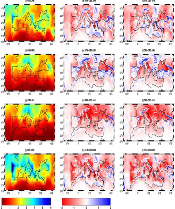
by Figure 7, which shows the seasonal climatology of the latent heatflux for observations (OA, first column) along with the biases for ATM (second column) and CPL (third column) experiments. Although both models overestimate the evaporation over the basin, mainly over Western Mediterranean, the coupling improves the simulation of evaporation over the Eastern Mediterranean in winter and spring and over most of the basin in fall. In summer, CPL is more evaporative than ATM over most of the Western Mediterranean. In summer and fall CPL is characterized by a decrease of latent heatflux over the northern part of the eastern basin and close to the Turkish coastlines. Finally, the mean sensible heatflux (Figure 6d) is equal to −13.18 W/m2 for ATM and −12.56 W/m2 for the CPL, which falls in the interval of OA ([−16; −10] W/m2) and Figure 7. As in Figure 4 but for observed (OA) net latent heatflux. Units are in W/m2.
NOCS ([−17; 2] W/m2) values, when taking into account the uncertainties associated with the data sets. We note that overall, and despite the biases discussed above, the model is capable of reproducing the seasonal and interannual variability of the quantities analyzed.
The heat fluxes shown in Figure 6 determine the total heat budget at the surface which, for the Mediterranean Sea, is negative and balanced by the inflow of Atlantic Water at the Gibraltar strait (Sevault et al., 2014, and references therein). Although it is not possible to compare the values of our budgets with long term estimates provided in the scientific literature due to the short length of our simulation, the value of the heat budget in CPL is equal to−0.26 W/m2which falls in the interval [−10; 0] W/m2for the period 1985–2004 discussed in Sevault et al. (2014) and references therein. The net inflow at the Gibraltar strait has been estimated for the period 2000–2006 equal to 0.07 Sv which falls in the interval of 0.04–0.1 Sv provided in Beuvier et al. (2010) and discussed in Sevault et al. (2014). Again, due to the limited length of the simulation it is not possible to provide a deeper insight into the water balance of the basin.
3.2. Ocean and Biogeochemistry 3.2.1. Oceanic Variables
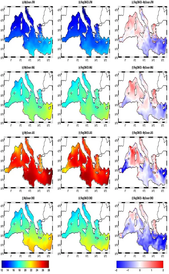
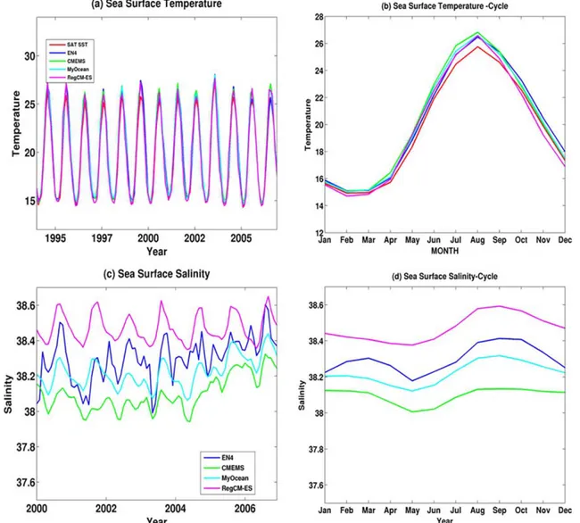
Figure 8 shows the seasonal climatology of SST according to MyOcean (Oddo et al., 2009; Pinardi et al., 2015; Simoncelli et al., 2019) and RegCM‐ES, along with associated biases, in JFM, AMJ, JAS and OND. RegCM‐ES reproduces well the SST spatial pattern in the basin with a clear north south gradient reflecting the spatial gradient in the shortwave radiation. RegCM‐ES tends to overestimate SST with respect to MyOcean mainly in spring and summer, especially over the western basin, a bias mostly likely due to the overestimation of shortwavefluxes during these seasons. Another contribution could originate from the coarse resolution of the atmospheric model (30 km) which is not able to reproduce correctly the intensity of local winds such as Mistral that has a cooling effect (Turuncoglu & Sannino, 2016). Conversely, RegCM‐ES has a negative bias (with a peak of −2°C) with respect to MyOcean in the eastern basin and in particular around the Cyprus area. Here, as shown in Turuncoglu and Sannino (2016), the intensity of winds simulated by the coupled model tends to be excessively strong, giving rise to colder than observed SST. Moreover, the colder SST in this area explain the strong positive and negative biases in evaporation and pre-cipitation, respectively, during the fall (Figures 5 and 7). In Figure 10 and Table 3 we compare SST and SSS mean values and variability in the Mediterranean Sea with some available observational and reanalysis data sets namely, the gridded Satellite SSTfield based on AVHRR measurements, covering the period 1981–2014 and described by Marullo et al. (2007), Nardelli et al. (2013), and Pisano et al. (2016); salinity and tempera-ture data set EN4, covering the period 1900–2015 and provided by the U.K. Met Office (Good et al., 2013); CMEMS, which covers the period 1955–2014 (Adani et al., 2011; Fratianni et al., 2015; Oddo et al., 2009; Simoncelli et al., 2016) and MyOcean, which covers the period 1987–2015 (Oddo et al., 2009; Pinardi et al., 2015; Simoncelli et al., 2019).
As shown in Table 3, the mean value of SST in the Mediterranean Sea during the period 1994–2006 is 19.81°C which is comparable with the values observed in the satellite data set (19.7°C) and slightly colder with respect to EN4 estimates (20.16°C) and in the two reanalysis products (20.26°C and 20.14°C for CMEMS and MyOcean, respectively). Taking into account the uncertainties in each data set the value reproduced by RegCM‐ES falls in the range of values of the satellite data set ([19.2; 20.15]°C), EN4 ([19.5; 20.8]°C), MyOcean ([19.5; 20.8]°C) and CMEMS ([19.4; 21.1]°C). Thus, on the basin scale, RegCM‐ES is characterized by an improvement in the SST biases from previous studies using Regional Earth System Models over the Mediterranean Sea (e.g., Artale et al., 2010; Sevault et al., 2014; Turuncoglu & Sannino, 2016). For example, the annual‐mean bias between CNRM‐RCSM4 and EN4 and CNRM‐RCSM4 and the satellite data set is −0.92°C and −0.60°C (Sevault et al., 2014) whereas in our case they are−0.35°C and 0.1°C, respectively. In JFM (Table 3), at the whole basin scale, RegCM‐ES is charac-terized by a cold bias of−0.3°C with respect to observations. This means a reduction in bias of ~1°C bias with respect to Protheus (Artale et al., 2010) and RegESM (Turuncoglu & Sannino, 2016). In JAS, RegCM‐ES tends to be slightly colder with respect to EN4, CMEMS and MyOcean (approximately [−0.2; −0.5]°C) and slightly warmer than satellite data (0.5°C). From this point of view the performance of RegCM‐ES in JAS and OND is comparable with that of Protheus and RegESM. Figures 10a and 10b shows that RegCM‐ES captures both the interannual and seasonal variability of SST in the basin, as well as the SST maximum that occurred during the long heat wave of summer 2003 and the two minima observed
Figure 8. Seasonal climatology of MyOcean SST (first column) in JFM (first row), AMJ (second row), JAS (third row), and OND (fourth row); RegCM‐ES SST (second column) and the related biases (third column) in the period
during the cold winters of 2004–2005 and 2005–2006 (Figure 10a). Concerning the seasonal cycle, RegCM‐ES captures the SST maximum in August and minimum in February, whose values are again in agreement with the reference data (Figure 10b).
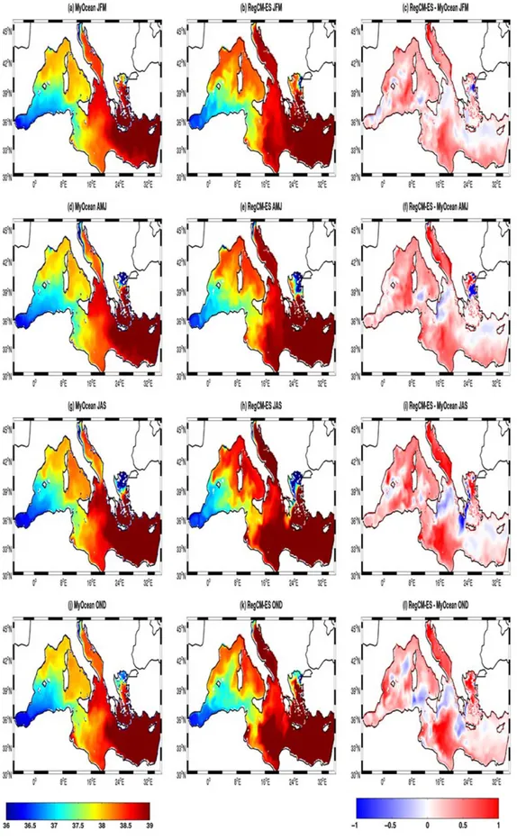
Figure 9 shows the corresponding analysis for SSS. RegCM‐ES is again able to capture the spatial patterns of SSS compared to the MyOcean reanalysis. On the other hand, at the basin scale the coupled model shows an Figure 10. Time series of net monthly averaged (first column) and annual cycle (second column) of SST (a, b, period 1994–2006) and SSS (c, d, 2000–2006): RegCM‐ES (magenta) for EN4 (blue), CMEMS (green), and MyOcean (cyan). Satellite SST are shown in red. Units are in °C and psu, respectively.
Table 3
Annual, Winter (JFM), and Summer (JAS) Mean Value for SST (Period 1994–2006) and SSS (2000–2006) Over the Mediterranean Sea in RegCM‐ES and Available Observational/Reanalysis Products (EN4, SST From Satellite, CMEMS, and MyOcean)
Data SST JFM SST JAS SST SSS JFM SSS JAS SSS
RegCM‐ES 19.8 15 25.5 38.47 38.42 38.55
EN4 20.16 [19.5; 20.8] 15.3 [14.7; 16] 25.7 [25.1; 26.3] 38.30 [38.11; 38.47] 38.27 [38.1; 38.45] 38.36 [38.13; 38.54] MyOcean 20.14 [19.5; 20.8] 15.3 [14.7; 16] 25.7 [25.1; 26.4] 38.22 [38.02; 38.42] 38.2 [38; 38.4] 38.3 [38.08; 38.48] CMEMS 20.26 [19.4; 21.1] 15.3 [14.7; 16.1] 26.02 [25.2; 26.84] 38.1 [37.84; 38.34] 38.12 [37.86; 38.37] 38.11 [37.86; 38.36] Satellite SST 19.7 [19.2; 20.15] 15.1 [14.6; 15.7] 24.94 [24.5; 25.3]
overestimation of SSS of about 0.25 and 0.38 psu with respect to the MyOcean and CMEMS reanalysis and 0.17 psu with respect to the EN4 observations. Specifically, the basin‐mean value of SSS (Table 3) in the per-iod 2000–2006 is equal to 38.47 psu, while for MyOcean and CMEMS the computed values are, respectively, equal to 38.22 and 38.10 psu, and 38.30 psu for EN4. Similar overestimations are also observed in JFM (approximately 0.15 psu with respect to EN4 and 0.2–0.3 psu with respect to CMEMS and MyOcean) and are more pronounced in JAS (approximately 0.19 psu with respect to EN4 and 0.3/0.4 psu with respect to CMEMS and MyOcean).
RegCM‐ES is characterized by positive biases in the Adriatic Sea, in the Western Mediterranean, and the Ionian Sea. These overestimations, particularly in summer, can have different origins (Sevault et al., 2014; Turuncoglu & Sannino, 2016), and include the underestimation of the river runoff computed by HD due to the relative coarse model grid (not shown here, Di Sante et al., 2019), the underestimation of precipitation over the Adriatic Sea in summer and over part of the basin in fall (as shown in Figure 5) and the overestima-tion of both evaporaoverestima-tion and shortwaveflux over the Western Mediterranean. Figure 10c compares the RegCM‐ES SSS monthly time series and annual cycle with the reference data sets. The model shows lower variability than observations (especially EN4) and, despite the aforementioned general overestimation, a good simulation of the annual SSS cycle.
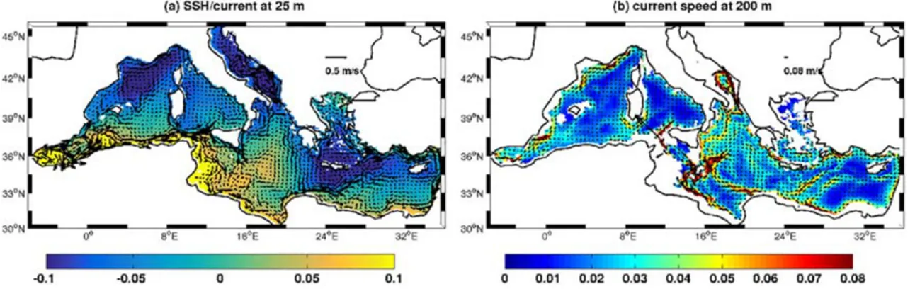
Figure 11a shows the mean dynamic sea surface height (SSH) and the mean circulation at 25 m (a) in the Mediterranean Sea for the period 2000–2006. The patterns for both variables are in good agreement with the results of previous studies (e.g., Pinardi et al., 2015; Sevault et al., 2014; Turuncoglu & Sannino, 2016). RegCM‐ES reproduces the flow of Atlantic Water through the Gibraltar Strait, the two anticyclonic gyres in the Alboran Sea and the Algerian current along the northern Africa coastline. As shown in Figure 11a, the Algerian current splits in two branches: One enters the Tyrrhenian Sea, whereas the other keepsflowing through the Sicily Channel then along the African coastlines reaching the Eastern Mediterranean and Anatolian coastlines, where it contributes to the Rhodes Gyre. In the Western Mediterranean, RegCM‐ES captures the negative SSH signal and the associated cyclonic circulation in the area of the Gulf of Lions and in the southern Adriatic, both markers of deep water formation processes (e.g., Pinardi et al., 2015; Sevault et al., 2014; Turuncoglu & Sannino, 2016). Figure 11b shows the mean circulation and current speed at 200 m. High values of current speed are shown south of Rhodes, in the Sicily Strait (Pierini & Rubino, 2001), along the African coastline (Pierini & Rubino, 2001), in the southern Adriatic, along the Gulf of Lions and toward the Gibraltar strait (as shown in Pinardi et al., 2015; Turuncoglu & Sannino, 2016). In summary, this analysis shows that RegCM‐ES is able to capture realistically the main fea-tures of the Mediterranean Sea surface and intermediate circulation.
3.2.2. Biogeochemical Variables
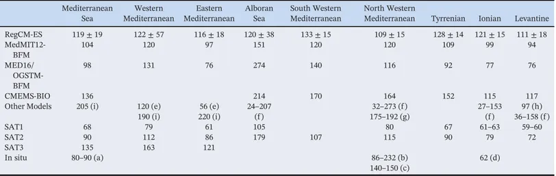
Table 4 compares the annual net primary production integrated over the top 200 m as simulated by RegCM‐ES for the period 2000–2006 with the available estimates. The net primary production is the rate of photosynthetic carbonfixation minus the fraction of fixed carbon used for cellular respiration (Boyd et al., 2014) and is one of the fundamental processes in the marine ecosystem. The simulation of this process is one of the greatest challenges in biogeochemical modeling. There are large differences in the values Figure 11. Mean sea surface height (SSH, contours) and the near‐surface/intermediate circulation field, at (a) 25 and (b) 200 m (arrows) as simulated by RegCM‐ES in the period 2000–2006. Units are in m for SSH and m/s for the velocity field.
estimated by different models and observations are characterized by pronounced uncertainties (Sein et al., 2015). Estimations shown in Table 4 are based on satellite products, in situ data and modeled data sets. The latter are taken from the hindcasts MED16/OGSTM‐BFM (Lazzari et al., 2012), MedMIT12‐BFM (Di Biagio et al., 2019) and CMEMS‐BIO (Teruzzi et al., 2016). In particular CMEMS‐BIO assimilates chlorophyll‐a satellite data in the first 10 m of the domain. The values in Table 4 represent averages over the full Mediterranean Sea and over the subdomains defined in Lazzari et al. (2012). The mean annual net primary production in RegCM‐ES (with the associated spatial standard deviation) across the Mediterranean Sea is 119 ± 20 gC/m2/year, with higher values in the western basin (122 ± 51 gC/m2/ year) compared to the eastern Basin (116 ± 18 gC/m2/year). These differences are consistent with the west‐east gradient in net primary production found in previous studies (Di Biagio et al., 2019; Lazzari et al., 2012; Teruzzi et al., 2016) and reported in Table 4. RegCM‐ES tends to show lower values of net primary production in the Alboran Sea and the north Western Mediterranean compared to MED16/OGSTM‐BFM, MedMIT12‐BFM, CMEMS‐BIO and SAT2. In the same regions, the RegCM‐ES values are in the range of the simulated and observational averages produced by Allen et al. (2002) and Marty and Chiaverini (2002). In south Western Mediterranean, the RegCM‐ES net primary production (133 ± 15 gC/m2/year) is in good agreement with the OGSTM‐BFM value of 140 gC/m2/year. On the other hand, the mean integrated primary production over the Tyrrhenian Sea and Ionian Sea, 128 ± 16 gC/m2/year and 121 ± 151 gC/m2/year, respectively, is higher than in MedMIT12‐BFM (109 and 99 gC/m2/year, respectively) and MED16/OGSTM‐BFM (97 and 77 gC/m2/year, respectively), but in better agreement with CMEMS‐BIO (152 gC/m2
/year for Tyrrhenian and 115 gC/m2/year for the Ionian) and Allen et al. (2002). Finally the mean net primary production value simulated in the Levantine Basin by RegCM‐ES, 111 ± 18 gC/m2/year, is in good agreement with estimate provided by CMEMS (117 gC/ m2/year) and in the range estimated by Allen et al. (2002) (36–158 gC/m2/year). Considering the large variability in the available estimates, RegCM‐ES reproduces realistic means and west‐east gradient of integrated net primary production over the Mediterranean basin.
Figure 12 and Table 5 compare mean surface chlorophyll‐a (averaged over the first 10 m) simulated by RegCM‐ES and averaged over the period 2000–2006 with MED16/OGSTM‐BFM (b, averaged over the period 1998–2004), CMEMS‐BIO (c, averaged over the period 2000–2006) and ESA satellite data (d, averaged over the period 2000–2006; Colella et al., 2016). The quantitive comparison in Table 5 includes also the modeled data set based on MedMIT12‐BFM (Di Biagio et al., 2019). Chlorophyll‐a concentration is a marker for phy-toplankton abundance and dynamics (e.g., Geider et al., 1997), which regulates the food chain of the marine ecosystems and modulates the CO2/O2concentration in the marine environment along with the exchanges
Table 4
Horizontal Means of the 0–200 m Integrated Net Primary Production (in Units of gC/m2/year) in the Mediterranean Sea and Related Subbasins as Annual Climatologies According to RegCM‐ES (With the Spatial Standard Deviation), Other Models, and Reference Data
Mediterranean Sea Western Mediterranean Eastern Mediterranean Alboran Sea South Western Mediterranean North Western
Mediterranean Tyrrenian Ionian Levantine
RegCM‐ES 119 ± 19 122 ± 57 116 ± 18 120 ± 38 133 ± 15 109 ± 15 128 ± 14 121 ± 15 111 ± 18 MedMIT12‐ BFM 104 120 97 151 120 120 109 99 94 MED16/ OGSTM‐ BFM 98 131 76 274 140 116 92 77 76 CMEMS‐BIO 136 214 170 164 152 115 117
Other Models 205 (i) 120 (e) 190 (i) 56 (e) 220 (i) 24–207 (f ) 32–273 (f) 175–192 (g) 27–153 (f ) 97 (h) 36–158 (f) SAT1 68 79 61 105 80 67 61–63 59–60 SAT2 90 112 86 179 107 115 90 79 72 SAT3 135 163 121 In situ 80–90 (a) 86–232 (b) 140–150 (c) 62 (d)
Note. MedMIT12‐BFM (Di Biagio et al., 2019), MED16/OGSTM‐BFM (Lazzari et al., 2012), CMEMS (Teruzzi et al., 2016), SAT1 (Uitz et al., 2012), SAT2 (Colella, 2007), and SAT3 (Bosc et al., 2004). In situ and other models: (a) Sournia (1973), (b) Marty and Chiaverini (2002), (c) Conan et al. (1998), (d) Boldrin et al. (2002), (e) Crispi et al. (2002), (f) Allen et al. (2002), (g) Kessouri et al. (2018), (h) Napolitano et al. (2000), and (i) Mattia et al. (2013).
with the overlying atmosphere. It is strongly dependent on sunlight/nutrients availability, with the latter depending on ocean vertical mixing and air‐sea interactions. Chlorophyll‐a is widely used and analyzed in many recent studies related to the biogeochemical modeling of the Mediterranean Sea (Di Biagio, 2017; Di Biagio et al., 2019; Lazzari et al., 2012; Mattia et al., 2013; Richon et al., 2017, 2018, 2019; Teruzzi et al., 2016; Valenti et al., 2017) due to the availability in the basin of both observational and modeled data sets.
RegCM‐ES captures the west‐east trophic gradient that characterizes the Mediterranean marine ecosystem, whose existence was emphasized in previous studies (D'Ortenzio & Ribera d'Alcala, 2009; Di Biagio et al., 2019; Lazzari et al., 2012; Mattia et al., 2013; Richon et al., 2017, 2018, 2019; Siokou‐Frangou et al., 2010; Salgado‐Hernanz et al., 2018). On the other hand, compared to the CMEMS‐BIO and satellite data, it under-estimates the signal of chlorophyll‐a at the mouth of the Mediterranean rivers and in the area of Gulf of Gabes. The source of this bias is traced to the lack of the model in nutrient discharge from coastal runoff in these regions and to a systematic positive bias which affects chlorophyll‐a satellite data in coastal regions associated with the presence of particulate matter (for instance, sediments) in the water column (Richon et al., 2019). RegCM‐ES captures the maximum of chlorophyll‐a in the gulf of Lions where, in the extended winter season JFMA, the simulated mean surface chl‐a is equal to 0.31 mg Chl/m3, comparable to 0.30 mg Chl/m3as observed in CMEMS‐BIO, as well as along the Adriatic coastline and in the Alboran Sea (D'Ortenzio & Ribera d'Alcala, 2009; Di Biagio, 2017; Di Biagio et al., 2019; Lazzari et al., 2012; Mattia et al., 2013; Richon et al., 2017; Richon et al., 2018, 2019; Salgado‐Hernanz et al., 2018). The signal observed in the Alboran Sea has been associated with the circulation pattern in the area (shown in Figure 11a), char-acterized by strong vertical velocities, which enriches the surface layer with nutrients triggering Figure 12. Mean chlorophyll‐a in the first 10 m in RegCM‐ES (a, averaged over the period 2000–2006), MED16/OGSTM‐ BFM (b, Lazzari et al., 2012, averaged over the period 1998–2004), CMEMS‐BIO (c, averaged over the period 2000–2006), and ESA satellite data (d, averaged over the period 2000–2006). Units are in mg Chl/m3.
Table 5
Horizontal Means of Chl‐a (in Units of mg/m3), PO4(in Units of mmol/m3), NO3(in Units of mmol/m3) and DOX (in Units of mmol/m3) in the Mediterranean Sea and Related Subbasins as Annual Climatologies in the First 150 m According to RegCM‐ES, Other Models, and Reference Data
Area Data set Chl‐a PO4 NO3 DOX
Mediterranean Sea RegCM‐ES 0.16 0.12 3.12 214
MedMIT12‐BFM 0.12 0.10 2.78 185
MED16/OGSTM‐BFM 0.08 0.04 1.33
CMEMS‐BIO 0.08 [0.04; 0.12] 0.04 [0.01; 0.07] 0.6 [0; 0.12] 210 [197; 223]
WOA18 0.12 [0.1; 0.14] 1.31 [1.06; 1.56] 235 [232; 238]
SAT 0.10
Western Mediterranean RegCM‐ES 0.20 0.16 3.58 217
MedMIT12‐BFM 0.16 0.15 3.35 187
MED16/OGSTM‐BFM 0.11 0.08 1.85
CMEMS‐BIO 0.12 0.07 1.12 205
WOA18 0.17 [0.15; 0.19] 2.30 [1.95; 2.65] 234 [231; 237]
SAT 0.15
Eastern Mediterranean RegCM‐ES 0.13 0.1 2.8 212
MedMIT12‐BFM 0.10 0.06 2.4 183
MED16/OGSTM‐BFM 0.05 0.02 0.95
CMEMS‐BIO 0.05 0.02 0.36 213
WOA18 0.09 [0.07; 0.11] 0.63 [0.43; 0.8] 236 [233; 239]
SAT 0.05
Alboran Sea RegCM‐ES 0.27 0.17 3.21 218
MedMIT12‐BFM 0.22 0.19 3.36 208
MED16/OGSTM‐BFM 0.23 0.14 1.63
CMEMS‐BIO 0.19 [0.05; 0.33] 0.09 [0.02; 0.16] 1.5 [0; 3.4] 153 [40; 193]
WOA18 0.22 [0.19; 0.25] 3.63 [3.23; 4.03] 224 [221; 227]
SAT 0.31
Southern Western Mediterranean RegCM‐ES 0.20 0.16 3.4 215
MedMIT12‐BFM 0.14 0.15 3.2 195
MED16/OGSTM‐BFM 0.10 0.08 1.5
CMEMS‐BIO 0.11 [0.09; 0.15] 0.07 [0.01; 0.15] 1 [0; 2] 200 [174; 223]
WOA18 0.13 [0.11; 0.15] 2 [1.8; 2.3] 234 [231; 238]
SAT 0.12
Northern Western Mediterranean RegCM‐ES 0.20 0.17 3.97 218
MedMIT12‐BFM 0.18 0.16 3.72 178
MED16/OGSTM‐BFM 0.13 0.08 2.3
CMEMS‐BIO 0.14 [0.07; 0.21] 0.08 [0; 0.18] 1.30 [0; 4.4] 214 [198; 233]
WOA18 0.20 [0.17; 0.23] 3 [2.7–3.4] 232 [230; 234]
SAT 0.17
Tyrrhenian RegCM‐ES 0.18 0.14 3.3 216
MedMIT12‐BFM 0.13 0.11 3.0 185
MED16/OGSTM‐BFM 0.08 0.05 1.63
CMEMS‐BIO 0.09 [0.04; 0.14] 0.06 [0.02; 0,10] 0.8 [0; 2.9] 214 [198; 230]
WOA18 0.14 [0.12; 0.16] 1.5 [1.3; 1.6] 238 [234; 242]
SAT 0.09
Ionian RegCM‐ES 0.14 0.1 2.85 213
MedMIT12‐BFM 0.10 0.07 2.54 185
MED16/OGSTM‐BFM 0.06 0.02 1.08
CMEMS‐BIO 0.06 [0.04; 0.08] 0.03 [0; 0.06] 0.4 [0; 1]. 214 [198; 230]
WOA18 0.07 [0.05; 0.09] 0.72 [0.5; 1] 236 [233; 239]
SAT 0.12
Levantine RegCM‐ES 0.12 0.09 2.7 211
MedMIT12‐BFM 0.08 0.05 2.2 182
MED16/OGSTM‐BFM 0.04 0.01 0.83
CMEMS‐BIO 0.05 [0.04; 0.06] 0.02 [0; 0.04] 0.3 [0; 1] 211 [195; 227]
WOA18 0.1 [0.08; 0.12] 0.53 [0.4; 0.6] 235 [233; 237]
SAT 0.05
Note. MedMIT12‐BFM (Di Biagio et al., 2019), MED16/OGSTM‐BFM (Lazzari et al., 2012; 2016), CMEMS‐BIO (Teruzzi et al., 2016), WOA18 (Garcia et al., 2018a, 2018b), and SAT (Colella et al., 2016). The values between brackets are the range of values of the reference data sets considering the uncertainties of the data (RMSD).
phytoplankton growth (Lazzari et al., 2012). The RegCM‐ES chlorophyll‐a signal observed in the gulf of Lionsfits in shape and size the minimum of SSH found over the area in Figure 11a, confirming the impor-tance of vertical mixing in enriching the upper layer of nutrients and driving the phytoplankton dynamics. However, RegCM‐ES generally tends to overestimate the chlorophyll‐a signal at the basin scale, in the Sicily Channel, Western Mediterranean (both western and southern parts), Tyrrhenian, Ionian, and Levantine basin (Table 5). In the Sicily channel the same maximum was observed in previous works (as Di Biagio, 2017; Di Biagio et al., 2019; Lazzari et al., 2012; Mattia et al., 2013) and was associated with enhanced vertical transport simulated by the model which enriches the surface with nutrients. The signal observed in the Western Mediterranean is likely associated with the overestimation of limiting phytoplankton growth nutrients (PO4and NO3) concentration in the water masses of the area with respect to CMEMS‐BIO data
set (as shown in Table 5).
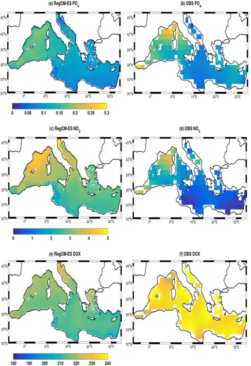
Figures 13a and 13b compare the simulated surface distribution of phosphate in the Mediterranean Sea to the observations from the World Ocean Atlas 2018 (WOA18, Garcia et al., 2018a, 2018b). RegCM‐ES cap-tures the low concentrations of phosphate within the Mediterranean Sea and the peculiar spatial west‐east gradient in this limiting nutrient, which is strictly correlated with the aforementioned gradient in the productivity (Lazzari et al., 2012; Richon et al., 2017, 2019, 2018). PO4values (Table 5) simulated by
RegCM‐ES are in good agreement with observations of WOA18 data set at the basin scale, in both Western and Eastern Mediterranean, in the Tyrrhenian Sea and Levantine basin. The same good level of agreement between model and reference data set is observed in the comparison with MedMIT12‐BFM data set in the Western Mediterranean, in the Alboran Sea, northern/southern Western Mediterranean, and Tyrrhenian Sea. However, the model underestimates the relatively high phosphate concentrations in the Alboran Sea, in the Gulf of Lions, and along the Ligurian coastlines (Figure 13 and Table 5). We ascribed this underestimation to a reduced vertical mixing induced by the Mistral wind in the coarse resolution atmo-spheric module (section 3.2.1) but also to the differences in the mean values of phosphate concentration in the Medar/Medatlas initial conditions which tends to be lower than 10% and than 50% with respect to WOA18 in the Alboran Sea and Gulf of Lions areas, respectively. At the basin scale and in all subbasins, both MedMIT12‐BFM and WOA18, together with RegCM‐ES, overestimates the mean concentration of phos-phate with respect to MED16/OGSTM‐BFM and CMEMS‐BIO.
The areas of Gulf of Lions, the northwestern Mediterranean, and the Alboran Sea show values of nitrate in good agreement with the values observed in WOA18 (Figures 13c and 13d and Table 5). RegCM‐ES repro-duces also the north‐south gradient in this dissolved nutrient already found in previous modeling studies (Lazzari et al., 2016). The same good level of agreement is observed again between RegCM‐ES and MedMIT12‐BFM at basin scale and in all subbasins (Table 5). However, compared to WOA18 data set, RegCM‐ES clearly simulates higher than observed values in the Tyrrhenian Sea, Ionian Sea, and the eastern basins (Figures 13c and 13d and Table 5). These differences are even stronger considering as reference data set CMEMS‐BIO and MED16/OGSTM‐BFM. Similar differences between model and observational data are obtained considering SiO4with RegCM‐ES simulating at least values of concentration two times higher with
respect to WOA18 (not shown). The tendencies of the model to simulate excess vertical mixing in the Tyrrhenian Sea and Levantine basin (Di Biagio et al., 2019), NO3values in the initial conditions which
are higher than those in the WOA18 data set of about 40% in the Ionian Sea and boundary biogeochemical conditions (more specifically river nutrients discharge and nutrients discharge at the Dardanelles Strait) can explain the differences between model and observations (D'Ortenzio et al., 2005; Di Biagio et al., 2019; Houpert et al., 2015).
For the dissolved oxygen RegCM‐ES tends to simulate lower (higher) values throughout the basin with respect to WOA18 (MedMIT12‐BFM, Table 5). On the other hand we observed a good level of agreement between RegCM‐ES and CMEMS‐BIO (Table 5) with the only exception of the Alboran Sea where differ-ences between the two values are originated from the different boundary conditions adopted in the two simulations. The misfit between WOA18 and modeled data can be traced mainly to the incorrect procedure adopted in the BFM Version 2 to convert the oxygen solubility values from ml/l to mmol/m3which erro-neously produces too low values (approximately 9%) with respect to the updated methodologies used in BFM Version 5. Version 2 of the BFM model is also adopted in the CMEMS‐BIO and this can explain the consistency between the two data sets (Table 5). Additional source of misfit between model and data are
the temperature and salinity biases between the two data sets which result in a lower oxygen solubility in RegCM‐ES mainly during the warm season (May‐June‐July‐August), with relatively larger negative values in the range [−5; −3]% in the northern Western Mediterranean, in the range [−4; −3]% in the southern West Mediterranean, in the range [−3; −2]% in the Tyrrhenian and Ionian Sea, and in the range [−2, 0]% in the Levantine basin.
Figure 14 compares qualitatively the vertical structure of chlorophyll‐a for the RegCM‐ES (a), MED16/OGSTM‐BFM (b) and CMEMS‐BIO (c) along a west‐east transect including the Alboran Sea, the Figure 13. Mean surface phosphate (a, b), nitrate (c, d), and dissolved oxygen (e, f ) concentration (first 150 m, in mmol/m3) simulated in the period 2000–2006 by RegCM‐ES (left column) compared to observations from the World Ocean Atlas (right column) 2018.
southwestern Mediterranean, the Ionian, and Levantine basins. This transect was described and used by D'Ortenzio and Ribera d'Alcala (2009), Lazzari et al. (2012), Di Biagio et al. (2019) to illustrate the chlorophyll‐a vertical structure in the basin and the location in the water column of the Deep Chlorophyll‐a Maximum (DCM). The figure shows that RegCM‐ES indeed captures this west‐east gradient in the vertical structure of chlorophyll‐a (D'Ortenzio & Ribera d'Alcala, 2009; Di Biagio et al., 2019; Lazzari et al., 2012; Moutin & Raimbault, 2002; Richon et al., 2017, 2018, 2019; Turley et al., 2000). Starting from the western portion of the transect, the DCM simulated by RegCM‐ES in the Alboran Sea is quite shallow (around 60 m), as in MED16/OGSTM‐BFM (b) and CMEMS (c), with a mean value of chlorophyll‐a of about 0.3 mg/m3. The same depth for DCM is observed moving eastward (up to 10°E, Lazzari et al., 2012). On the other hand, in the Ionian and Levantine basin the model tends to reproduce a shallower DCM than that observed in the two modeled data sets, with higher values of chlorophyll‐a. In fact, while for RegCM‐ES the DCM is located around 80–90 m, in MED16/OGSTM‐BFM and CMEMS it is located around 100–110 m. The differences between RegCM‐ES and CMEMS‐BIO can be mostly attributed to the vertical ocean mixing scheme, which tends to overestimate vertical mixing in some areas of the basins with respect to reanalysis, such as the Strait of Sicily and the Levantine basin. This process enriches the upper layer with nutrients favoring phytoplankton growth and higher surface chlorophyll‐a concentrations in a shallower DCM.
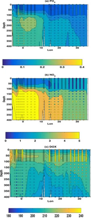
The vertical distribution of phosphate, nitrate and dissolved oxygen simulated by RegCM‐ES along the same transect adopted for chlorophyll‐a (Figure 14a) is compared with WOA18 data in Figure 15. As discussed in the introduction, the vertical structure of nutrients is strongly influenced by both physical (e.g., estuarine inverse circulation) and biogeochemical processes (e.g., the biological pump). The representation of realistic oxygenfields in a physical biogeochemical model is critical because of the ecological importance of dissolved oxygen concentration and its sensitivity to climatic perturbations. The phytoplankton is an important source Figure 14. Vertical section from the Gibraltar strait to the Levantine Basin of the averaged chlorophyll‐a: RegCM‐ES (a, 2000–2006), MED16/OGSTM‐BFM (b, Lazzari et al., 2012; 1998–2004), and CMEMS‐BIO (c, 2000–2006). Units are in mg Chl/m3.