New results on path-decompositions
and their down-links
A. Benini, L. Giuzzi and A. Pasotti
∗Abstract
In [3] the concept of down-link from a (Kv,Γ)-design B to a
(Kn,Γ′)-design B′ has been introduced. In the present paper the
spectrum problems for Γ′ = P
4 are studied. General results on
the existence of decompositions and embeddings between path-decompositions playing a fundamental role for the construction of down-links are also presented.
Keywords: (Kv,Γ)-design; down-link; embedding.
MSC(2010): 05C51, 05B30, 05C38.
1
Introduction
Suppose Γ ≤ K to be a subgraph of K. A (K, Γ)-design, or Γ-decomposition of K, is a set of graphs isomorphic to Γ whose edges partition the edge set of K. Given a graph Γ, the problem of determining the existence of (Kv,
Γ)-designs, also called Γ-designs of order v, where Kv is the complete graph
on v vertices, has been extensively studied; see the surveys [4, 5]. In [3] we proposed the following definition.
Definition 1.1. Given a (K, Γ)-design B and a (K′,Γ′)-design B′ with
Γ′ ≤ Γ, a down-link from B to B′ is a function f ∶ B → B′ such that
f(B) ≤ B, for any B ∈ B.
When such a function f exists, we say that it is possible to down-link Bto B′.
∗[email protected], [email protected], [email protected],
Dipar-timento di Matematica, Facolt`a di Ingegneria, Universit`a degli Studi di Brescia, Via Valotti 9, I-25133 Brescia (IT).
The present research was performed within the activity of GNSAGA of the Italian INDAM with the financial support of the Italian Ministry MIUR, projects “Strutture di incidenza e combinatorie” and “Disegni combinatorici, grafi e loro applicazioni”.
As seen in [3], down-links are closely related to metamorphoses [8], their generalizations [9] and embeddings [11]. In close analogy to embeddings, we introduced spectrum problems about down-links:
(I) For each admissible v, determine the set L1Γ(v) of all integers n such
that there exists some Γ-design of order v down-linked to a Γ′-design of order n.
(II) For each admissible v, determine the set L2Γ(v) of all integers n such
that every Γ-design of order v can be down-linked to a Γ′-design of
order n.
In [3, Proposition 3.2], we proved that for any v such that there exists a (Kv,Γ)-design and any Γ′≤ Γ, the sets L1Γ(v) and L2Γ(v) are always
non-empty. In the same paper the case Γ′= P
3 has been investigated in detail.
Here we shall deal with the case Γ′ = P
4. In order to get results about
down-links to P4-designs, we shall first study path-designs and their
embed-dings. More precisely, in Section 2 we determine sufficient conditions for the existence of P4-decompositions of any graph Γ and Pk-decompositions
of complete bipartite graphs. In Section 3, applying the results of Section 2, we are able to prove the existence of embeddings and down-links be-tween path-designs. Section 4 is devoted to the cases of cycle systems and path-designs, with general theorems and directed constructions.
Throughout this paper the following standard notations will be used; see also [7]. For any graph Γ, write V (Γ) for the set of its vertices and E(Γ) for the set of its edges. If B is a collection of graphs, by V (B) we will mean the set of the vertices of all its elements. By tΓ we shall denote the disjoint union of t copies of graphs all isomorphic to Γ. As usual, Pk=[a1, . . . , ak]
is the path with k − 1 edges and Ck =(a1, . . . , ak), k ≥ 3, is the cycle of
length k. Also, Km,n is the complete bipartite graph with parts of size m
and n. When we focus on the actual parts X and Y , KX,Y will be written.
2
Existence of some path-designs
In this section we present new results on the existence of path decompo-sitions. Recall that a (Kn, Pk)-design exists if, and only if, n(n − 1) ≡ 0
(mod 2(k − 1)); see [13].
Proposition 2.1. Let k be an even integer. For x = k − 2, k the complete bipartite graph Kk−1,x admits a Pk-decomposition.
Proof. Consider the bipartite graph KA,I where A = {a1, . . . , ak−1} and
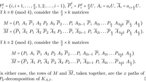
I={1,... ,x} with x = k − 2,k. Let Ut=(1,... ,1) be an x 2-tuple. Set P t 1 =(1,... ,x2) and for i = 1,... , x 2,
Pit=(i,i + 1,... ,x
2,1, 2, . . . , i − 1), P t
i= Pit+x2U, Ai= aiU, Ai= ai+k 2U.
If k ≡ 0 (mod 4), consider the x
2× kmatrices M =(P1 A1 P1 A2 P2 A3 P2. . . Pi A2i−1 Pi A2i. . . Pk 4 A k−2 2 P k 4 A k 2) M =(P1 A1 P1 A2 P2A3 P2. . . PiA2i−1Pi A2i. . . Pk 4 A k−2 2 P k 4 A k 2).
If k ≡ 2 (mod 4), consider the x
2× kmatrices M =(P1 A1 P1A2P2 A3 P2. . . Pi A2i−1 Pi A2i. . . Pk+2 4 A k 2) M =(P1A1 P1A2P2 A3 P2. . . Pi A2i−1 Pi A2i. . . Pk+2 4 A k 2).
In either case, the rows of M and M , taken together, are the x paths of a Pk-decomposition of KA,I.
Theorem 2.2. Let Γ be a graph with at least two vertices of degree∣V (Γ)∣−1. Then Γ admits a P4-decomposition if, and only if, ∣E(Γ)∣ ≡ 0 (mod 3). If
∣E(Γ)∣ ≡ 1,2 (mod 3), then Γ can be partitioned into a P4-decomposition
together with one or two (possibly connected) edges, respectively.
Proof. The condition is obviously necessary. For sufficiency, let α and β be two vertices of degree∣V (Γ)∣ − 1. Delete α and β in Γ, as to obtain a graph G. Let G′be a maximal P
4-decomposable subgraph of G and remove
from G the edges of G′, determining a new graph G′′. In general, G′′ is
not connected and its connected components are either isolated vertices or stars or cycles of length 3; call I, S and C their (possibly empty) sets. Let Γ′ be the graph obtained removing the edges of G′ from Γ. Clearly, ∣E(Γ)∣ ≡ 0 (mod 3) implies ∣E(Γ′)∣ ≡ 0 (mod 3); thus it remains to show
that E(Γ′) is P4-decomposable. Obviously α and β are of degree∣V (Γ)∣−1
also in Γ′. Let A ={α,β} and consider the following decomposition Γ′=
KA∪KA,I∪(C∪KA,V(C))∪(S∪KA,V(S)). We begin by providing, separately,
P4-decompositions of KA,I, C ∪ KA,V(C) and S ∪ KA,V(S).
i) It is easy to see that for any 3-subset of I, say H3, the graph KA,H3
has a P4-decomposition. Thus, depending on the congruence class modulo
3 of∣I∣, KA,Ican be partitioned into a P4-decomposition together with the
following possible remnants.
(i1) ∣I∣ ≡ 0 (mod 3) (i2) ∣I∣ ≡ 1 (mod 3) (i3) ∣I∣ ≡ 2 (mod 3)
the set ∅ the path [α, h, β] the cycle (h1, α, h2, β)
with h ∈ I with h1, h2∈ I
ii) For any 3-cycle C ∈ C, the graph C ∪KA,V(C)has a P4-decomposition.
Thus, C ∪ KA,V(C) also admits a P4-decomposition.
iii) It is not difficult to see that, for any star Sc∈ S of center c, the graph
Sc∪ KA,V(Sc) has a partition into a P4-decomposition together with either
the path[α,c,β] or the graph (α,c,β,v) ∪ [c,v], where v is any external vertex, depending on whether the number of vertices of Sc is odd or even.
Let S1 (respectively S2) be the set of stars with an odd (even) number of
vertices. For any three stars of S1(S2) the remnants give P4-decomposable
graphs. So S1∪ KA,V(S1), as well as S2∪ KA,V(S2), can be partitioned into
a P4-decomposition together with the possible remnants outlined in Tables
2 and 3.
(iii11) (iii12) (iii13)
∣S1∣ ≡ 0 (mod 3) ∣S1∣ ≡ 1 (mod 3) ∣S1∣ ≡ 2 (mod 3)
the path [α, c, β] the cycle (c1, α, c2, β)
∅ where where
cis the center of a star c1, c2 are centers of two stars
Table 2: Case iii1: S1∪ KA,V(S1).
(iii21) (iii22) (iii23)
∣S2∣ ≡ 0 (mod 3) ∣S2∣ ≡ 1 (mod 3) ∣S2∣ ≡ 2 (mod 3)
the graph the graph
(α, c, β, v) ∪ [c, v] ⋃2i=1(α, ci, β, vi) ∪ [ci, vi]
∅ where c is the center where c1, c2 are centers
and v is an external vertex and v1, v2 are external vertices
of a star of two stars
Table 3: Case iii2: S2∪ KA,V(S2).
The remnants from i), iii1) and iii2) together with the edge [α,β] can be
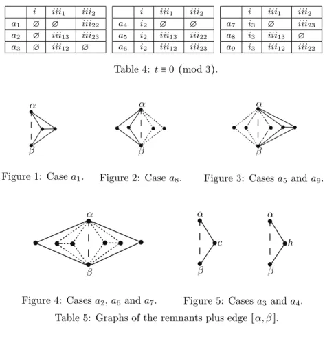
combined in 27 different ways to obtain 27 connected graphs with t edges. It is a routine to check that we have exactly 9 cases with t ≡ i (mod 3), for i= 0, 1, 2.
In Table 4 we will list in detail the 9 cases with t ≡ 0 (mod 3) and, for each of them, in Table 5 we give the corresponding graph.
i iii1 iii2 a1 ∅ ∅ iii22 a2 ∅ iii13 iii23 a3 ∅ iii12 ∅ i iii1 iii2 a4 i2 ∅ ∅ a5 i2 iii13 iii22 a6 i2 iii12 iii23 i iii1 iii2 a7 i3 ∅ iii23 a8 i3 iii13 ∅ a9 i3 iii12 iii22 Table 4: t ≡ 0 (mod 3). α β Figure 1: Case a1. α β Figure 2: Case a8. α β
Figure 3: Cases a5 and a9.
α
β
Figure 4: Cases a2, a6 and a7.
α β c α β h
Figure 5: Cases a3and a4.
Table 5: Graphs of the remnants plus edge[α,β].
It is easy to determine a P4-decomposition of the graphs in Figures 1, 2, 3,
4. In cases a3 and a4(Figure 5) a P4-decomposition is clearly not possible,
thus we proceed back tracking one step in the construction. How to deal with case a3 is explained in Figure 6.
α
β c
v1 v2 Figure 6: We recover the two P4’s from 2 radii of the
star of center c.
In case a4we have to distinguish several subcases depending on the size of
α β a h h1 h2
h3 Figure 7: If ∣I∣ > 1, we recover the two P4’s from 3
vertices of I. α β b1 b2 b3
h Figure 8: If∣I∣ = 1 and ∣C∣ ≠ 0 we recover the three P4’s from a C3.
When∣I∣ = 1 and ∣C∣ = 0 we have two possibilities. If there is one star of S with at least two edges, we proceed as explained in Figure 9.
α
β c v1
v2 h Figure 9: If∣I∣ = 1, ∣C∣ = 0, and ∃Sc∈ S with P3≤ Sc
we recover the two P4’s from 2 radii of Sc.
Otherwise, G′′ consists of an isolated vertex h and a set P of disjoint P2’s.
Since ∣E(Γ′)∣ ≡ 0 (mod 3), the size of P is also divisible by 3, let ∣P∣ = 3p.
It is easy to see that for any 3-subset of P, say P3, the graph K
A,P3 has a
P4-decomposition. After p − 1 steps, the remnant is the graph in Figure 10,
which likewise admits a P4-decomposition. This concludes the case t ≡ 0
(mod 3). α
β
h Figure 10: If∣I∣ = 1, ∣C∣ = 0 and S is a disjoint union of P2’s we recover the 15 edges from the last but one
step.
With similar arguments, when t ≡ 1, 2 (mod 3) it is possible to find a P4
3
Embeddings and down-links to P
4-designs
The results presented in the previous section are used to prove the existence of embeddings and down-links to path designs. In particular, we shall focus our attention on P4-decompositions.
Theorem 3.1. Any partial(Kv, P4)-design can be embedded into a (Kn, P4
)-design for any admissible n ≥ v + 2.
Proof. Let B be a partial(Kv, P4)-design. Let A be a set of vertices disjoint
from V(Kv) with v + ∣A∣ ≡ 0,1 (mod 3) and ∣A∣ ≥ 2. Let Γ be the graph
such that V(Γ) = V (Kv) ∪ A and E(Γ) = E(Kv+∣A∣) ∖ E(B). Since ∣A∣ ≥ 2,
by Theorem 2.2 there exists a (Γ,P4)-design B′ and, clearly, B ∪ B′ is a
(Kv+∣A∣,P4)-design.
Corollary 3.2. For any(Kv,Γ)-design with P4≤ Γ
{n ≥ v + 2 ∣ n ≡ 0,1 (mod 3)} ⊆ L2Γ(v) ⊆ L1Γ(v).
Proof. Let B be a(Kv,Γ)-design with P4≤ Γ. Choose a P4in each block of
Band call P the set of such P4’s. Obviously, P is a partial P4-decomposition of Kv. Hence, by Theorem 3.1, P can be embedded into a(Kn, P4)-design
B′ for any admissible n ≥ v + 2. The construction also guarantees the existence of a down-link from B to B′.
Theorem 3.3. For any even integer k, a Pk-design of order n ≡ 0, 1(modk−
1) can be embedded into a Pk-design of any order m > n + 1 with m ≡
0, 1(modk − 1).
Proof. Let B be a (Kn, Pk)-design with n ≡ 0,1 (mod k − 1) and let m =
n + s≡ 0, 1(modk − 1). As Kn+s = Kn∪ Ks∪ Kn,s, for the existence of a
(Km, Pk)-design embedding B it is enough to find a Pk-decomposition of
Ks∪ Kn,s. Since n, n + s ≡ 0, 1(modk − 1), one of the following cases occurs
• n = λ(k − 1),s = µ(k − 1) ⇒ Ks⋃Kn,s= Ks⋃λµKk−1,k−1 • n = λ(k−1),s = 1+µ(k−1) ⇒ Ks⋃Kn,s= Ks⋃Kλ(k−1),k+(µ−1)(k−1)= = Ks⋃λKk−1,k⋃λ(µ − 1)Kk−1,k−1 • n = 1+λ(k−1),s = µ(k−1) ⇒ Ks⋃Kn,s= Ks⋃Kk+(λ−1)(k−1),µ(k−1)= = Ks⋃µKk,k−1⋃µ(λ − 1)Kk−1,k−1 • n = 1 + λ(k −1),s = k −2 +µ(k −1) ⇒ Ks⋃Kn,s= Ks⋃K1+λ(k−1),s= = Ks⋃K1,s⋃Kλ(k−1),s= Ks+1⋃Kλ(k−1),k−2+µ(k−1)= = Ks+1⋃λKk−1,k−2⋃λµKk−1,k−1
So, to find a Pk-decomposition of Ks∪ Kn,s it is sufficient to know Pk
• Ksand Ks+1, which exist by [13],
• Kk−1,k−1, whose existence is proved in [10],
• Kk−1,kand Kk−1,k−2, whose existence follows from Proposition 2.1.
The following corollary is a straightforward consequence of Theorem 3.3. Corollary 3.4. If n ∈ LiΓ(v), then
{m ≥ n + 2 ∣ m ≡ 0,1(mod3)} ⊆ LiΓ(v).
Remark 3.5. Set ηi = inf LiΓ(v). By Corollary 3.4, LiΓ(v) contains all
admissible values m ≥ ηiapart from (possibly) ηi+1. Thus to exactly
deter-mine the spectra it is enough to compute ηi and ascertain if ηi+1 ∈ LiΓ(v).
4
Cycle systems and path-designs
Here we shall provide some partial results on the existence of down-links from cycle systems and path-designs to P4-designs.
We recall that a k-cycle system of order v, that is a(Kv, Ck)-design, exists
if, and only if, k ≤ v, v is odd and v(v − 1) ≡ 0 (mod 2k); see [2], [12]. Theorem 4.1. For any admissible v and any k ≥ 9
{n ≥ v − ⌊k −49⌋ ∣ n ≡ 0,1 (mod3)} ⊆ L2Ck(v) ⊆ L1Ck(v).
Proof. Let k ≥ 9 and let B be a(Kv, Ck)-design. Write t = ⌊k−94 ⌋. Take t+2
distinct vertices x1, x2, . . . , xt, y1, y2 ∈ V(Kv). Observe that it is possible
to extract from each block C ∈ B a P4 whose vertices are different from
x1, x2, . . . , xt, y1, y2, as we are forbidding at most 4(t + 1) + 2 = 4t + 6 = k − 3
edges from any k-cycle. Use these P4’s for the down-link. Let S be the
image of the down-link, considered as a subgraph of Kv−t= Kv∖{x1, . . . , xt}
and remove the edges of S from Kv−t to obtain a new graph R. It remains
to show that R admits a P4-decomposition. Observe that∣V (R)∣ = v−t and
y1, y2 are two vertices of R of degree v − t − 1. To apply Theorem 2.2 we
have to distinguish some cases according to the congruence class modulo 3 of v − t.
If v − t ≡ 0(mod 3), then ∣E(R)∣ ≡ 0(mod 3) so the existence of a (R,P4
)-design is guaranteed by Theorem 2.2. Furthermore, if we add a vertex to Kv−t we can apply Theorem 2.2 also to R′ = R ∪ K1,v−t since ∣E(R′)∣ ≡
to(Kv−t+1, P4)-designs.
If v − t ≡ 1(mod 3), then ∣E(R)∣ ≡ 0(mod 3), hence by Theorem 2.2, there exists a(R,P4)-design. So we determine down-links from B to (Kv−t, P4
)-designs.
Finally, if v−t ≡ 2(mod 3), it is sufficient to add either u = 1 or u = 2 vertices to Kv−t and then apply Theorem 2.2 to R′′=(Kv−t∪ Ku∪ Kv−t,u) ∖ S in
order to down-link B to (Kv−t+1, P4)-designs or to (Kv−t+2, P4)-designs,
respectively. The statement follows from Remark 3.5.
Arguing exactly as in the previous proof it is possible to prove the following result.
Theorem 4.2. For any admissible v and any k ≥ 12 {n ≥ v − ⌊k −12
4 ⌋ ∣n ≡ 0,1 (mod3)} ⊆ L2Pk(v) ⊆ L1Pk(v).
4.1
Small cases
We shall now investigate in detail the spectrum problems for Γ = C4 and
Γ = P5. In order to obtain our results, we shall extensively use the method
of gluing of down-links, introduced in [3]. We briefly recall the main idea: a down-link from a(Kv,Γ)-design to a (Kn,Γ′)-design can be constructed
as union of down-links between partitions of the domain and the codomain. To give designs suitable for the down-link, we will use difference families; here we recall some preliminaries, for a survey see [1]. Let Γ be a graph. A set F of graphs isomorphic to Γ with vertices in Zv is called a
(v,Γ,1)-difference family (DF, for short) if the list ∆F of (v,Γ,1)-differences from F , namely the list of all possible differences x − y, where (x,y) is an ordered pair of adjacent vertices of an element of F , covers Zv∖{0} exactly once. In [6]
it is proved that if F ={B1, . . . , Bt} is a (v,Γ,1)-DF, then the collection of
graphs B ={Bi+ g∣ Bi∈ F , g ∈ Zv} is a cyclic (Kv,Γ)-design.
Lemma 4.3. For any v ≡ 1, 9 (mod 24), v > 1, there exists a down-link from a (Kv, C4)-design to a (Kv, P4)-design. For any v ≡ 9,17 (mod 24)
there exists a down-link from a(Kv, C4)-design to a (Kv+1, P4)-design.
Proof. Take v = s + 24t ≥ 9, with s = 1, 9, 17, and V(Kv) = Zv. Consider the
set of 4-cycles C={Ca=(0,a,v +1 2 , v −1 8 + a) ∣ a = 1,2,... , v −1 8 } . It is straightforward to check that
∆Ca= ±{a,v +1 2 − a, 3v + 5 8 − a, v −1 8 + a}.
Hence ∆C = Zv∖{0}, so, by [6], the Ca are the v−18 base blocks of a cyclic
(Kv, C4)-design. The development of each base block gives v different
4-cycles, from each of which we extract the edge obtained by developing[0,a]. The obtained P4’s will be used to define a down-link in a natural way. The
removed edges can be connected to complete the P4-decomposition of Kv
as follows: for each triple{[0,a + 1],[0,a + 2],[0,a + 3]}, for a ≡ 1 (mod 3) where a ∈{1,2,...,v−1
8 }, consider the three developments and connect the
edges{[i + 1,a + 1 + (i + 1)],[i,a + 2 + i],[i,a + 3 + i]} obtaining the paths (i + 1,a + i + 2,i,a + i + 3), with i ∈ Zv.
If v ≡ 1 (mod 24), we have the required P4-decomposition.
If v ≡ 9 (mod 24), we have the required P4-decomposition except for the
development of [0,1]. The v edges of such a development can be easily connected to give the v-cycle C =(0,1,... ,v − 1), which obviously admits a P4-decomposition. So, for v ≡ 1, 9 (mod 24), there exists a down-link
from a (Kv, C4)-design to a (Kv, P4)-design. Under the assumption v ≡ 9
(mod 24), n = v + 1 is also admissible. In this case, add the vertex α to V(Kv) to obtain a Kv+1 supporting the codomain of the down-link.
Actually, the star S[α;V ] of center α and external vertices the elements of
V(Kv) has been added. Proceed as before till to the last but one step,
namely do not decompose the v-cycle C obtained by developing [0,1]. So it remains to determine a P4-decomposition of the wheel W = C ∪ S[α;V ].
It is easy to see that W can be decomposed into 3 + 8t copies of the graph W′in Figure 11, which evidently admits a P4-decomposition.
Figure 11: The graph W′as union of two P4’s.
If v ≡ 17 (mod 24), proceeding as before, we determine the required P4
-decomposition except for the two developments, say d1and d2, of the edges
[0,1] and [0,v−1
8 ]. Keeping in mind that we must also add a vertex, say α,
to the codomain, we have to arrange the edges of d1, d2and S[α;V ]. It easy
to see that we can obtain the P4’s as[α,1 + i,i,v−18 + i], for i ∈ Zv.
So, for v ≡ 9, 17 (mod 24) there exists a down-link from a (Kv, C4)-design
Theorem 4.4. For any admissible v > 1,
L1C4(v) = {n ≥ v ∣ n ≡ 0,1 (mod3)}; (1)
{n ≥ v + 2 ∣ n ≡ 0,1 (mod3)} ⊆ L2C4(v) ⊆ {n ≥ v ∣ n ≡ 0,1 (mod3)}. (2)
Proof. Let B and B′ be, respectively, a (K
v, C4)-design and a (Kn, P4
)-design. Suppose that B can be down-linked to B′. Clearly, n ≥ v. Hence
L2C4(v) ⊆ L1C4(v) ⊆ {n ≥ v ∣ n ≡ 0,1 (mod 3)}.
To prove the reverse inclusion in (1) observe that a (Kv, C4)-design exists
if, and only if, v ≡ 1 (mod 8) and a (Kn, P4)-design exists if, and only
if, n ≡ 0, 1 (mod 3). So it makes sense to look for a down-link from a (Kv, C4)-design to a (Kv, P4)-design only for v ≡ 1,9 (mod 24). Likewise,
a down-link from a(Kv, C4)-design to a (Kv+1, P4)-design can exist only if
v≡ 9, 17 (mod 24). The existence of such down-links is proved in Lemma 4.3. The statement of (1) follows from Remark 3.5. The other inclusion in (2) immediately follows from Corollary 3.2.
Theorem 4.5. For any admissible v > 1,
L1P5(v) = {n ≥ v − 1 ∣ n ≡ 0,1(mod3)}; (3)
{n ≥ v + 2 ∣ n ≡ 0,1(mod3)} ⊆ L2P5(v) ⊆ {n ≥ v ∣ n ≡ 0,1(mod3)}. (4)
Proof. The first inclusion in (4) follows from Corollary 3.2. In order to prove the second, it is sufficient to show that for any admissible v there exists a (Kv, P5)-design B wherein no vertices can be deleted. In particular, this
is the case if each vertex of Kv has degree 2 in at least one block of B.
First of all note that in a(Kv, P5)-design there is at most one vertex with
degree 1 in each block where it appears. Suppose that there actually exists a (Kv, P5)-design B with a vertex x as above. It is easy to see that in
B there is at least one block P1 =[x,a,b,c,d] such that the vertices a,b
and c have degree two in at least another block. Let P2 = [x,d,e,f,g].
By reassembling the edges of P1∪ P2, it is possible to replace in B these
two paths with P3 = [d,x,a,b,c], P4 = [c,d,e,f,g] if c ≠ f,g or P5 =
[a,x,d,c,g],P6=[a,b,c,e,d] if c = f or P7=[c,d,x,a,b],P8=[b,c,f,e,d]
if c = g. Thus we have again a(Kv, P5)-design. By the assumption on a,b,c
all the vertices of this new design have degree two in at least one block. Now we consider Relation (3). Let B and B′ be respectively a (Kv, P5
)-design and a(Kn, P4)-design. Suppose there exists a down-link f ∶ B → B′.
Clearly, n > v − 2. Hence, L1P5(v) ⊆ {n ≥ v − 1 ∣ n ≡ 0,1(mod3)}.
To show the reverse inclusion in (3) we prove the actual existence of designs providing down-links. Since a (Kv, P5)-design exists if, and only if, v ≡
0, 1(mod8) and a (Kn, P4)-design exists if, and only if, n ≡ 0,1(mod3), it
makes sense to look for a down-link from a(Kv, P5)-design to a (Kv−1, P4
to construct a down-link from a(Kv, P5)-design to a (Kv, P4)-design only
for v ≡ 0, 1, 9, 16(mod24). In view of Remark 3.5, in order to complete the proof, we have also to provide a down-link from a(Kv, P5)-design to a
(Kv+1, P4)-design for every v ≡ 0,9(mod24).
To determine the necessary down-links, we analyze a few basic cases and then apply the gluing method. To this end, we will use the following obvious relations in an appropriate way: Ka+b= Ka⋃Kb⋃Ka,band Ka+b,c= Ka,c∪
Kb,c. In particular, Kℓ+24t = Kℓ∪ K24t∪ Kℓ,24t; K24t = tK24∪( t 2)K24,24= tK24∪48( t 2)K3,4; Kℓ=rs,24t = rKs,24t= rtKs,24= 6rtKs,4= 8rtKs,3.
Let us now examine the possible cases.
●(Kv, P5) → (Kv−1, P4)-design with v = ℓ + 24t > 1, ℓ = 1,8,16,17.
P5-design basic components → basic components P4-design
of order of order 1 + 24t (K25, P5), (K3,4, P5) (K24, P4), (K3,4, P4) 24t 8 + 24t (K8, P5), (K24, P5) (K7, P4), (K24, P4) 7 + 24t (K4,3, P5) (K4,3, P4), (K3,3, P4) 16 + 24t (K16, P5), (K24, P5) (K15, P4), (K24, P4) 15 + 24t (K4,3, P5) (K4,3, P4), (K3,3, P4) 17 + 24t (K17, P5), (K24, P5) (K16, P4), (K24, P4) 16 + 24t (K4,3, P5) (K4,3, P4), (K3,3, P4) ●(Kv, P5) → (Kv, P4)-design with v = ℓ + 24t > 1, ℓ = 0,1,9,16.
P5-design basic components → basic components P4-design
of order of order 24t (K24, P5), (K3,4, P5) (K24, P4), (K3,4, P4) 24t 1 + 24t (K9, P5), (K16, P5) (K9, P4), (K16, P4) 1 + 24t (K24, P5),(K3,4, P5) (K24, P4),(K3,4, P4) 9 + 24t (K9, P5), (K24, P5) (K9, P4), (K24, P4) 9 + 24t (K3,4, P5) (K3,4, P4) 16 + 24t (K16, P5), (K24, P5) (K16, P4), (K24, P4) 16 + 24t (K3,4, P5) (K3,4, P4) ●(Kv, P5) → (Kv+1, P4)-design with v = ℓ + 24t > 1, ℓ = 0,9.
P5-design basic components → basic components P4-design
of order of order
24t (K24, P5), (K3,4, P5) (K25, P4), (K3,4, P4) 1 + 24t
9 + 24t (K9, P5), (K24, P5) (K10, P4), (K24, P4) 10 + 24t
It is straightforward to show the existence of such basic down-links. For in-stance we provide a down-link ξ from a(K9,24, P5)-design to a (K10,24, P4
)-design. Let A = {a,b,c,d,e,f,g,h,i} and B = Z24, that is K9,24 = KA,B.
The following are the 54 paths of a P5-decomposition of KA,B: [6, a, 12, b, 1] [1, c, 12, d, 6] [6, e, 18, f, 1] [1, g, 12, h, 0] [12, i, 0, a, 18] [7, a, 13, b, 2] [2, c, 13, d, 7] [7, e, 19, f, 2] [2, g, 13, h, 1] [13, i, 1, a, 19] [8, a, 14, b, 3] [3, c, 14, d, 8] [8, e, 20, f, 3] [3, g, 14, h, 2] [14, i, 2, a, 20] [9, a, 15, b, 4] [4, c, 15, d, 9] [9, e, 21, f, 4] [4, g, 15, h, 3] [15, i, 3, a, 21] [10, a, 16, b, 5] [5, c, 16, d, 10] [10, e, 22, f, 5] [5, g, 16, h, 4] [16, i, 4, a, 22] [11, a, 17, b, 0] [0, c, 17, d, 11] [11, e, 23, f, 0] [0, g, 17, h, 5] [17, i, 5, a, 23] [18, b, 6, c, 19] [19, d, 0, e, 12] [12, f, 6, g, 19] [19, h, 6, i, 18] [19, b, 7, c, 20] [20, d, 1, e, 13] [13, f, 7, g, 20] [20, h, 7, i, 19] [20, b, 8, c, 21] [21, d, 2, e, 14] [14, f, 8, g, 21] [21, h, 8, i, 20] [21, b, 9, c, 22] [22, d, 3, e, 15] [15, f, 9, g, 22] [22, h, 9, i, 21] [22, b, 10, c, 23] [23, d, 4, e, 16] [16, f, 10, g, 23] [23, h, 10, i, 22] [23, b, 11, c, 18] [18, d, 5, e, 17] [17, f, 11, g, 18] [18, h, 11, i, 23].
We obtain the image of any P5 via ξ by removing the underlined edge.
Now, to complete the codomain, we have to add a further vertex to A, say α, together with all the edges connecting α to the vertices of B. Thus, it remains to decompose the graph formed by the removed edges together with the star of center α and external vertices in B. Such a P4-decomposition is
listed below: [6, a, 9, α] [7, a, 10, α] [8, a, 11, α] [1, c, 4, α] [2, c, 5, α] [3, c, 0, α] [9, e, 6, α] [10, e, 7, α] [11, e, 8, α] [4, g, 1, α] [5, g, 2, α] [0, g, 3, α] [15, i, 12, α] [16, i, 13, α] [17, i, 14, α] [22, d, 19, α] [23, d, 20, α] [21, d, 18, α] [12, f, 15, α] [13, f, 16, α] [14, f, 17, α] [20, h, 21, α] [23, h, 22, α] [20, b, 23, α] [h, 18, b, 21] [h, 19, b, 22].
References
[1] Abel, R.J.R., Buratti, M., Difference families, in: CRC Handbook of Combinatorial Designs (C.J. Colbourn and J.H. Dinitz eds.), CRC Press, Boca Raton, FL (2006), 392–409.
[2] Alspach, B., Gavlas, H., Cycle decompositions of Kn and Kn− I, J.
Combin. Theory Ser. B 81 (2001), 77–99.
[3] Benini, A., Giuzzi, L., Pasotti, A., Down-linking (Kv,Γ)-designs to
P3-designs, to appear on Util. Math. (arXiv:1004.4127).
[4] Bos´ak, J., “Decompositions of graphs”, Mathematics and its Appli-cations (1990), Kluwer Academic Publishers Group.
[5] Bryant, D., El-Zanati, S., Graph Decompositions, CRC Handbook of Combinatorial Designs, C.J. Colbourn and J.H. Dinitz, CRC Press (2006), 477–486.
[6] Buratti, M., Pasotti, A., Graph decompositions with the use of differ-ence matrices, Bull. Inst. Combin. Appl. 47 (2006), 23–32.
[7] Harary, F., “Graph Theory” (1969), Addison-Wesley.
[8] Lindner, C.C., Rosa, A., The metamorphosis of λ-fold block designs with block size four into λ-fold triple systems, J. Stat. Plann. Inference 106 (2002), 69–76.
[9] Ling, A.C.H., Milici, S., Quattrocchi, G., Two generalizations of the metamorphosis definition, Bull. Inst. Combin. Appl. 43 (2005), 58– 66.
[10] Parker, C. A., Complete bipartite graph path decompositions, Ph.D. Thesis, Auburn University (1998).
[11] Quattrocchi, G., Embedding G1-designs into G2-designs, a short
sur-vey, Rend. Sem. Mat. Messina Ser. II 8 (2001), 129–143.
[12] ˜Sajna, M., Cycle decompositions III: complete graphs and fixed length cycles, J. Combin. Designs 10 (2002), 27–78.
[13] Tarsi, M., Decomposition of a complete multigraph into simple paths: nonbalanced handcuffed designs, J. Combin. Theory Ser. A 34 (1983), 60–70.