Scuola di Dottorato in Ingegneria “Leonardo da Vinci”
Corso di Dottorato di Ricerca in
Ingegneria dell’Informazione
SSD ING-INF/03
Tesi di Dottorato di Ricerca
Advanced Techniques for Detecting Anomalies
in Backbone Networks
Autore:
Teresa Pepe
Relatori:
Prof. Stefano Giordano
Prof. Michele Pagano
Copyright c Teresa Pepe, 2012
All rights reserved
Manuscript received February 28, 2012
Accepted March 28, 2012
Sommario
Con il rapido sviluppo e la crescente complessit`a delle reti di com-puter, i meccanismi tradizionali di network security non riescono a fornire soluzioni dinamiche e integrate adatte a garantire la completa sicurezza di un sistema. In questo contesto, l’uso di sistemi per la rile-vazione delle intrusioni (Intrusion Detection System - IDS) `e diventato un elemento chiave nell’ambito della sicurezza delle reti.
In questo lavoro di tesi affrontiamo tale problematica, proponendo soluzioni innovative per l’intrusion detection, basate sull’uso di tec-niche statistiche (Wavelet Aanalysis, Principal Component Analysis, etc.) la cui applicazione per la rilevazione delle anomalie nel traffico di rete, risulta del tutto originale.
L’analisi dei risultati presentata, in questo lavoro di tesi, evidenzia l’efficacia dei metodi proposti.
Abstract
With the rapid development and the increasing complexity of com-puter and communication systems and networks, traditional security technologies and measures can not meet the demand for integrated and dynamic security solutions. In this scenario, the use of Intrusion Detection Systems has emerged as a key element in network security. In this thesis we address the problem considering some novel statisti-cal techniques (e.g., Wavelet Analysis, Principal Component Analysis, etc.) for detecting anomalies in network traffic.
The performance analysis, presented in this work, shows the effec-tiveness of the proposed methods.
Contents
List of figures x
List of tables xii
List of acronyms xiv
Introduction 1
1 Intrusion Detection System 5
1.1 Network security . . . 5
1.1.1 The OSI security architecture . . . 6
1.2 Intrusion Detection Systems . . . 14
1.2.1 IDS taxonomy . . . 19
1.3 Abilene/Internet2 Network . . . 22
2 Sketch data model 25 2.1 Sketch . . . 25
2.1.1 Data streaming model . . . 25
2.1.2 Sketch . . . 26
2.1.3 Reversible Sketch . . . 28
vi CONTENTS
3 Principal Component Analysis 41
3.1 Pricipal Component Analysis . . . 41
3.2 System architecture . . . 44 3.2.1 Flow Aggregation . . . 45 3.2.2 Time-series Construction . . . 46 3.2.3 Anomaly Detector . . . 48 3.2.4 Identification . . . 51 3.3 Experimental results . . . 53 3.3.1 Traffic aggregations . . . 56 3.3.2 KL divergence . . . 62 4 Wavelet Analysis 67 4.1 Wavelet Decomposition and Multiresolution Analysis . 67 4.2 System architecture . . . 70 4.2.1 Anomaly Detector . . . 73 4.2.2 Identification . . . 75 4.3 Experimental results . . . 75 5 Change Detection 83 5.1 Change-Point Detection . . . 83
5.1.1 Cumulative Sum control chart(CUSUM) . . . . 84
5.2 Streaming Change Detection . . . 86
5.2.1 Heavy Hitter Detection . . . 87
5.2.2 Heavy Change Detection . . . 87
5.3 System architecture . . . 88
5.3.1 Anomaly Detector . . . 90
5.3.2 Identification . . . 98
CONTENTS vii
6 Wave-CUSUM - combining Wavelet and CUSUM 111
6.1 Wavelet Pre-Filtering . . . 111 6.2 System Architecture . . . 118 6.2.1 Wavelet Module . . . 120 6.2.2 Detection Module . . . 120 6.2.3 Identification phase . . . 121 6.3 Experimental results . . . 122 7 Conclusions 131 Bibliography 137
List of Figures
1.1 IDS - hybrid architecture . . . 21
1.2 Abilene/Internet2 Network . . . 22
2.1 Sketch - Update Function . . . 27
2.2 Modular Hashing . . . 29
2.3 IP Mangling - Distribution of number of keys for each bucket . . . 32
2.4 Reverse hashing procedure (example) . . . 40
3.1 PCs of a two-dimentional dataset . . . 42
3.2 Scree Plot . . . 44
3.3 PCA - System Architecture . . . 45
3.4 PCA - Data matrix . . . 51
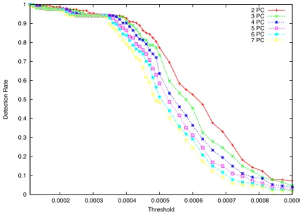
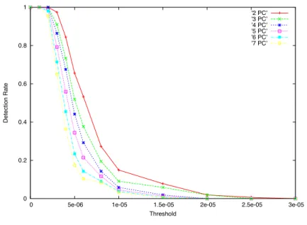
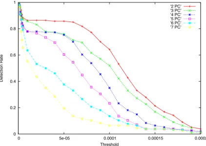
3.5 PCA - Detection Rate vs. Number of PCs . . . 54
3.6 PCA - Detection Rate vs. Sketch Size . . . 55
3.7 PCA - Detection Rate for OD traffic aggregation . . . 57
3.8 PCA - Detected Anomalies for OD traffic aggregation 58 3.9 PCA - Detection Rate for IR traffic aggregation . . . . 59
3.10 PCA - Detected Anomalies for IR traffic aggregation . 60 3.11 PCA - Detection Rate for IL traffic aggregation . . . . 61 3.12 PCA - Detected Anomalies for IL traffic aggregation . 62
x LIST OF FIGURES
3.13 PCA - Detection Rate for Random Aggregation . . . . 63
3.14 PCA - Detected Anomalies for Random Aggregation . 64 3.15 PCA - Detected Anomalies - KL divergence . . . 65
3.16 PCA - Detection Rate - KL divergence . . . 66
4.1 Daubechies mother wavelet . . . 69
4.2 Wavelet Decomposition . . . 70
4.3 Wavelet - System architecture . . . 72
4.4 Wavelet Analysis . . . 74
4.5 Wavelet - Distance - Original Traces . . . 77
4.6 Wavelet - Distance - Traces with artificial anomalies . 78 4.7 Wavelet - Number of detected attacks . . . 79
4.8 Heavy Change Detection: number of detected attacks 80 4.9 Wavelet - Detection rate . . . 81
5.1 Intuitive derivation of the CUSUM: time series (upper graph) and CUSUM statistics (lower graph) . . . 85
5.2 Change Detection - System Architecture . . . 89
6.1 Wavelet Decomposition . . . 112
6.2 Original Signal (traffic aggregate over one week) . . . 114
6.3 Reconstructed Signal - Low-frequency Component . . 115
6.4 Reconstructed Signal - Mid-frequency Component . . 116
6.5 Reconstructed Signal - High-frequency Component . . 117
6.6 Wave-CUSUM - System Architecture . . . 119
6.7 Wave-CUSUM - Reconstructed Signal . . . 123
List of Tables
3.1 PCA - Detection Rate vs. Anomalous Time-Bins . . . 60 3.2 PCA - Kl-entropy Additive Detections . . . 64 4.1 Wavelet - Notations . . . 71 5.1 Change Detection - Method 1 . . . 99 5.2 Change Detection - Method 2 (w = 256, EWMA α =
0.2, JSD) . . . 100 5.3 Change Detection - Method 2 (w = 512, EWMA α =
0.2, JSD) . . . 100 5.4 Change Detection - Method 2 (w = 1024, EWMA α =
0.2, JSD) . . . 101 5.5 Change Detection - Method 2 (w = 512, EWMA α =
0.5, JSD) . . . 103 5.6 Change Detection - Method 2 (w = 512, EWMA α =
0.8, JSD) . . . 103 5.7 Change Detection - Method 2 ( w = 512, NSHW α =
0.2 β = 0.2, JSD) . . . 105 5.8 Change Detection - Method 2 ( w = 512, NSHW α =
xii LIST OF TABLES 5.9 Change Detection - Method 2 ( w = 512, NSHW α =
0.2 β = 0.8, JSD) . . . 106
5.10 Change Detection - Method 2 (w = 512, no forecasting, JSD) . . . 107
5.11 Change Detection - Method 2 (w = 512, EWMA α = 0.2, KL) . . . 108
5.12 Change Detection - Method 3 . . . 110
6.1 Wave-CUSUM - low volume anomalies . . . 125
6.2 CUSUM - low volume anomalies . . . 126
6.3 Wave-CUSUM - medium volume anomalies . . . 127
6.4 CUSUM - medium volume anomalies . . . 127
6.5 Wave-CUSUM - high volume anomalies . . . 128
List of Acronyms
CUSUM Cumulative Sum
CWT Continuous Wavelet Transform
DDoS Distributed Denial of Service
DoS Denial of Service
DWT Discrete Wavelet Transform
EWMA Exponential Weighted Moving Average
GF Galois Field
HC Heavy Change
HH Heavy Hitter
HIDS Host-based IDS
IDES Intrusion Detection Expert System
IDS Intrusion Detection System
IP Internet Protocol
ITU-T International Telecommunication Union Telecommunication standardization sector
JSD Jensen-Shannon Divergence
KL Kullback-Leibler divergenge
xiv LIST OF ACRONYMS
NSHW Non Seasonal Holt-Winters
NIDS Network-based IDS
OS Operating System
OSI Open Systems Interoperability
PC Principal Component
PCA Principal Component Analysis
Introduction
With the rapid development and the increasing complexity of com-puter and communication systems and networks, traditional security technologies and measures can not meet the demand for integrated and dynamic security solutions. Moreover, along with the prolifera-tion of new services, the threats from spammers, attackers and crim-inal enterprises also grow.
Recent advances in encryption, public key exchange, digital signa-ture, and the development of related standards have set a foundation for network security. However, security on a network goes beyond these issues. Indeed it must include security of computer systems and networks, at all levels, top to bottom.
Since it seems impossible to guarantee complete protection to a sys-tem by means of prevention mechanisms (e.g., authentication tech-niques and data encryption), the use of an Intrusion Detection System (IDS) is of primary importance to reveal intrusions in a network or in a system.
State of the art in the field of intrusion detection is mostly rep-resented by misuse based IDSs that are designed to detect known attacks by utilizing the signatures of those attacks. Considering that most attacks are realized with known tools, available on the Internet, a signature based IDS could seem a good solution. Nevertheless such
2 Introduction systems require frequent rule-base updates and signature updates, and are not capable of detecting unknown attacks.
In contrast, anomaly detection systems, a subset of IDSs, model the normal system/network behavior, which enables them to be extremely effective in finding and foiling both known as well as unknown or zero day attacks. This is the main reason why our work focuses on the development of an anomaly based IDS.
In particular we propose several novel statistical methods to be used for the description of the “normal” behavior of the network traffic. In more detail we explore the use of Wavelet Analysis, Principal Compo-nent Analysis, as well as techniques for Change-Point Detection and Heavy Hitter Detection.
All the proposed Anomaly based IDSs work on the top of a proba-bilistic structure, namely the sketch, that allows a random aggregation of the data, so as to obtain a more scalable system.
The remainder of this work is organized as follows: Chapter 1 is devoted to the description of the fundamentals of network security, mainly focusing on the description of the statistical Intrusion Detec-tion Systems.
Chapter 2 presents some theoretical background on the sketch data model, used in this work as a common substrate for all the proposed systems.
The subsequent four chapters, namely Chapter 3, 4, 5, and 6, are dedicated to the detailed discussion of the implemented methods. In more detail Chapter 3, at first provides a quick overview of the the-oretical background about Principal Component Analysis and then discusses the system architecture and the experimental results.
Anal-Introduction 3 ogously Chapter 4 is devoted to the presentation of the architecture of the system based on the Wavelet Analysis, as well as of the achieved performance. Chapter 5 provides an overview of the Change Detec-tion algorithms used by the implemented system (CUSUM, Heavy Hitter and Heavy Change detection algorithms) and then details the architecture and the performance of the system. Then Chapter 6 dis-cusses both the architecture and the performance of a system based on a combined use of Wavelet Analysis and CUSUM.
Chapter 1
Intrusion Detection
System
1.1
Network security
In the field of networking the area of network security [1] [2] usually refers to a complex process, which involves mechanisms and services necessary to guarantee the security of the information in a distributed context (e.g., the Internet).
The main objective of this process is to define a security policy that the network administrator can adopt to prevent and monitor unautho-rized access, misuse, modification, or denial of the computer network and network-accessible resources.
To perform such operations it is necessary to keep in mind three important concepts:
• Absolute security can not be guaranteed: any system can be compromised, at least, by means of a brute-force attack 1
1
A brute force attack is a method of defeating a security scheme by trying a large number of possibilities; for example, exhaustively working through all possible
6 Intrusion Detection System • Security asymptotically improves: securing a system is not a
cost-less operation. Thus, it is necessary to attentively perform a risk evaluation phase
• Security and easiness are opposite concepts: adding security mechanisms to a system implies adding complexity
When talking about network security, there mainly exist two stan-dard documents: RFC 2828 titled “Internet Security Glossary” [3] and the recommendation X.800 by ITU-T [4]. In the following sec-tions we describe the architecture presented in X.800, only referring to [3] in some special cases.
1.1.1 The OSI security architecture
ITU-T recommendation X.800 defines a systematic approach to the security problems. For our purposes, the OSI security architecture provides a useful, if abstract, overview of many of the security con-cepts. The OSI security architecture focuses on security attacks, mechanisms, and services. These can be defined briefly as follows:
• Security attack: any action that compromises the security of information owned by an organization
• Security mechanism: a process (or a device incorporating such a process) that is designed to detect, prevent, or recover from a security attack
• Security service: a processing or communication service that enhances the security of the data processing systems and the keys in order to decrypt a message
1.1 Network security 7 information transfers of an organization. The services are in-tended to counter security attacks, and they make use of one or more security mechanisms to provide the service
In the following we present, in more detail, each of these concepts. Security services
X.800 defines a security service as a service provided by a protocol layer of communicating open systems, which ensures adequate security of the systems or of data transfers. Perhaps a clearer definition is found in [3], which provides the following definition: “a processing or communication service that is provided by a system to give a specific kind of protection to system resources; security services implement security policies and are implemented by security mechanisms”.
X.800 divides these services into five categories and fourteen specific services:
• Authentication: the authentication service is concerned with assuring that a communication is authentic. In the case of a single message, such as a warning or alarm signal, the function of the authentication service is to assure the recipient that the message is from the source that it claims to be from. In the case of an ongoing interaction, such as the connection of a terminal to a host, two aspects are involved. First, at the time of connection initiation, the service assures that the two entities are authentic, that is, that each is the entity that it claims to be. Second, the service must assure that the connection is not interfered with in such a way that a third party can masquerade as one of the two
8 Intrusion Detection System legitimate parties for the purposes of unauthorized transmission or reception. Two specific authentication services are defined in X.800:
– Peer entity authentication: used in association with a log-ical connection to provide confidence in the identity of the entities connected
– Data-origin authentication: in a connectionless transfer, provides assurance that the source of received data is as claimed
• Access control: in the context of network security, access con-trol is the ability to limit and concon-trol the access to host systems and applications via communications links. To achieve this, each entity trying to gain access must first be identified, or authen-ticated, so that access rights can be tailored to the individual • Data confidentiality: confidentiality is the protection of
trans-mitted data from passive attacks. With respect to the content of a data transmission, several levels of protection can be iden-tified:
– Connection confidentiality: the protection of all user data on a connection
– Connectionless confidentiality: the protection of all user data in a single data block
– Selective-field confidentiality: the confidentiality of selected fields within the user data on a connection or in a single data block
1.1 Network security 9 – Traffic-flow confidentiality: the protection of the
informa-tion that might be derived from observainforma-tion of traffic flows • Data integrity: as with confidentiality, integrity can apply to a stream of messages, a single message, or selected fields within a message. Again, the most useful and straightforward approach is total stream protection. As in the previous case, several types of data integrity are defined in X.800:
– Connection integrity with recovery: provides for the in-tegrity of all user data on a connection and detects any modification, insertion, deletion, or replay of any data within an entire data sequence, with recovery attempted
– Connection integrity without recovery: as above, but pro-vides only detection without recovery
– Selective-field connection integrity: provides for the in-tegrity of selected fields within the user data of a data block and takes the form of determination of whether the selected fields have been modified, inserted, deleted, or re-played
– Connectionless integrity: provides for the integrity of a sin-gle connectionless data block and may take the form of de-tection of data modification. Additionally, a limited form of replay detection may be provided
– Selective-field connectionless integrity: provides for the in-tegrity of selected fields within a single connectionless data block; takes the form of determination of whether the se-lected fields have been modified
10 Intrusion Detection System • Nonrepudiation: nonrepudiation prevents either sender or
re-ceiver from denying a transmitted message
– Nonrepudiation, origin: proves that the message was sent by the specified party
– Nonrepudiation, destination : proves that the message was received by the specified party
• Availability: availability is the property of a system or a sys-tem resource being accessible and usable upon demand by an authorized system entity, according to performance specifica-tions for the system.
It is worth noticing that X.800 treats availability as a property to be associated with various security services. However, it makes sense to call out specifically an availability service. An availabil-ity service is one that protects a system to ensure its availabilavailabil-ity. This service addresses the security concerns raised by denial-of-service attacks. It depends on proper management and control of system resources and thus depends on access control service and other security services.
Security mechanisms
In the following we describe the security mechanisms defined in X.800. As can be seen the mechanisms are divided into those that are imple-mented in a specific protocol layer and those that are not specific to any particular protocol layer or security service.
1.1 Network security 11 appropriate protocol layer in order to provide some of the OSI security services
– Encipherment: the use of mathematical algorithms to trans-form data into a trans-form that is not readily intelligible. The transformation and subsequent recovery of the data depend on an algorithm and zero or more encryption keys
– Digital signature: data appended to, or a cryptographic transformation of, a data unit that allows a recipient of the data unit to prove the source and integrity of the data unit and protect against forgery
– Access control: a variety of mechanisms that enforce access rights to resources
– Data integrity: a variety of mechanisms used to assure the integrity of a data unit or stream of data units
– Authentication exchange: a mechanism intended to ensure the identity of an entity by means of information exchange – Traffic padding: the insertion of bits into gaps in a data
stream to frustrate traffic analysis attempts
– Routing control: enables selection of particular physically secure routes for certain data and allows routing changes, especially when a breach of security is suspected
– Notarization: the use of a trusted third party to assure certain properties of a data exchange
• Pervasive security mechanisms: mechanisms that are not specific to any particular OSI security service or protocol layer
12 Intrusion Detection System – Trusted functionality: that which is perceived to be
cor-rect with respect to some criteria (e.g., as established by a security policy)
– Security label: the marking bound to a resource (which may be a data unit) that names or designates the security attributes of that resource
– Event detection: detection of security-relevant events – Security audit trail: data collected and potentially used to
facilitate a security audit, which is an independent review and examination of system records and activities
– Security recovery: deals with requests from mechanisms, such as event handling and management functions, and takes recovery actions
Security Attacks
In the literature, the terms threat and attack are commonly used to mean more or less the same thing. But, RFC 2828, defines this two concept in a different way:
• Threat: a potential for violation of security, which exists when there is a circumstance, capability, action, or event that could breach security and cause harm. That is, a threat is a possible danger that might exploit a vulnerability
• Attack: an assault on system security that derives from an intelligent threat; that is, an intelligent act that is a deliberate attempt (especially in the sense of a method or technique) to evade security services and violate the security policy of a system
1.1 Network security 13 Regarding the attacks, X.800 defines several specific attacks, divided into passive and active:
• Active attacks: active attacks involve some modification of the data stream or the creation of a false stream and can be subdivided into four categories:
– Masquerade: one entity pretends to be a different entity – Replay: involves the passive capture of a data unit and
its subsequent retransmission to produce an unauthorized effect
– Modification of messages: simply means that some portion of a legitimate message is altered, or that messages are delayed or reordered, to produce an unauthorized effect – Denial of Service (DoS): prevents or inhibits the normal
use or management of communications facilities
• Passive attacks: passive attacks are in the nature of eaves-dropping on, or monitoring of, transmissions. The goal of the opponent is to obtain information that is being transmitted. Passive attacks are very difficult to detect because they do not involve any alteration of the data. Typically, the message traffic is sent and received in an apparently normal fashion and neither the sender nor receiver is aware that a third party has read the messages or observed the traffic pattern.Two types of passive attacks are:
– Release of message content: we would like to prevent an opponent from learning the contents of a data transmission
14 Intrusion Detection System – Traffic Analysis: traffic analysis, is a subtler type of
at-tack. Suppose that we had a way of masking the contents of messages or other information traffic so that opponents, even if they captured the message, could not extract the information from the message. The common technique for masking contents is encryption. If we had encryption pro-tection in place, an opponent might still be able to observe the pattern of these messages. The opponent could deter-mine the location and identity of communicating hosts and could observe the frequency and length of messages being exchanged. This information might be useful in guessing the nature of the communication that was taking place
1.2
Intrusion Detection Systems
Since, inevitably, the best intrusion prevention system will fail, we need a mechanism which should act when an intrusion occurs. For this reason the IDS has been the focus of much research in recent years.
Definition 1 An IDS is a software or hardware tool aimed at detect-ing unauthorized access to a computer system or a network.
In other word, an intrusion detection is the act of detecting actions that attempt to compromise the confidentiality, integrity or availabil-ity of a system/network.
The attention IDSs have had is motivated by several considerations, including the following:
1.2 Intrusion Detection Systems 15 • If an intrusion is detected quickly enough, the intruder can be
identified and ejected from the system before any damage is done or any data are compromised. Even if the detection is not sufficiently timely to preempt the intruder, the sooner the intrusion is detected, the less the amount of damage and the more quickly recovery can be achieved
• An effective IDS can serve as a deterrent, so acting to prevent intrusions
• Intrusion detection enables the collection of information about intrusion techniques that can be used to strengthen the intrusion prevention facility
Intrusion detection is based on the assumption that the behavior of intruder significantly differs from that of a legitimate user.
The concept of IDS was first introduced by Anderson in the early 80s [5]. The idea was to perform a post-processing of the audit data produced by a machine, so as to reveal if any intrusion had been carried out. The main flaw of this kind of system is that the detection was performed off-line.
For this reason, 1987 is usually considered as birth date of the IDSs, when Denning in [6] introduced her Intrusion Detection Expert Sys-tem (IDES).
The main characteristic of IDES is to be independent of any partic-ular system, application environment, system vulnerability, or type of intrusion. IDES is, in fact, a framework for a general-purpose IDS. Moreover, one of the most relevant feature of IDES is that it intro-duces the idea of performing the detection of intrusions by means of
16 Intrusion Detection System a statistical analysis of the system input data. Thus, roughly speak-ing, the working of the system is based on the characterization of the behavior of a subject, with respect to a given object, by means of a statistical profile. An intrusion is revealed if such a profile is not respected by the input data.
In more detail, the model has six main components:
• Subjects: subjects are the initiators of actions in the target system. A subject is typically a terminal user, but might also be a process acting on behalf of users or groups of users, or might be the system itself. Subjects can be grouped into classes by type (groups may overlap)
• Objects: objects are the receptors of actions and typically in-clude such entities as files, programs, messages, records, termi-nals, printers, and user- or program-created structures. When subjects can be recipients of actions (e.g., electronic mail), then those subjects are also considered to be objects in the model. Objects can be grouped into classes by type
• Audit records: generated by the target system in response to actions performed or attempted by subjects on objects-user login, command execution, file access, and so on
• Profiles: structures that characterize the behavior of a given subject (or set of subjects) with respect to a given object (or set thereof), thereby serving as a signature or description of normal activity for its respective subject and object. Observed behavior is characterized in terms of a statistical metric and
1.2 Intrusion Detection Systems 17 model. A metric is a random variable x representing a quanti-tative measure accumulated over a period. The period may be a fixed interval of time, or the time between two audit-related events. Observations xi of x obtained from the audit records
are used together with a statistical model to determine whether a new observation is abnormal. The statistical model makes no assumptions about the underlying distribution of x; all knowl-edge about x is obtained from observations. In more detail the metric can be:
– Event Counter: x is the number of audit records satisfying some property occurring during a period of time
– Interval Timer: x is the length of time between two related events
– Resource Measure: x is the quantity of resources consumed by some action during a period as specified in the Resource-Usage field of the audit records
Instead, the statistical model can be:
– Operational model: this model is based on the operational assumption that abnormality can be decided by comparing a new observation of x against fixed limits. Although the previous sample points for x are not used, presumably the limits are determined from prior observations of the same type of variable
– Mean and standard deviation model: this model is based on the assumption that all we know about x1, x2, . . . , xn,
18 Intrusion Detection System are mean and standard deviation. A new observation xn+1
is defined to be abnormal if it falls outside a confidence interval
– Multivariate model: this model is similar to the mean and standard deviation model except that it is based on corre-lations among two or more metrics
– Markov process model: this model, which applies only to event counters, regards each distinct type of event as a state variable, and uses a state transition matrix to char-acterize the transition frequencies between states. A new observation is defined to be abnormal if its probability as determined by the previous state and the transition matrix is too low
– Time series model: this model, which uses an interval timer together with an event counter or resource measure, takes into account the order and interarrival times of the ob-servations x1, x2, . . . , xn, as well as their values. A new
observation is abnormal if its probability of occurring at that time is too low
• Anomaly records: generated when abnormal behavior is de-tected
• Activity rules: actions taken when some condition is satisfied, which update profiles, detect abnormal behavior, relate anoma-lies to suspected intrusions, and produce reports
1.2 Intrusion Detection Systems 19
1.2.1 IDS taxonomy
IDSs are usually classified on the basis of several aspects, in the follow-ing we describe the most important categories of these systems [7] [8].
Host-based IDS vs. Network-based IDS
A first distinction is usually made between host-based IDS (HIDS) and network-based IDS (NIDS). The main difference between these two categories is given by the input data of the system: a HIDS mainly processes the operating system’s logs, while a NIDS processes the network traffic.
As a consequence of that, the first class of IDSs reveals those attacks, towards a single host, that leave some traces in the host’s audit files. It should be clear that the most relevant limitation of this approach is given by the fact that these systems strongly depend on the OS. This fact usually takes to a low level of interoperability among different systems.
On the contrary, the NIDSs, processing low level data, do not depend on the hosts architecture. Moreover, these system are able to detect attacks that do not affect the system log files and can protect an entire LAN rather than a single host.
Stateless IDS vs. Stateful IDS
The second distinction we present, between stateful and stateless IDSs, is based on the approach, used to process the input data. A stateless system processes each event of the input data independently of the previous and the following events. On the contrary a stateful
20 Intrusion Detection System IDS considers each event of the input data, as part of a stream of events. Thus the IDS decisions do not only depend on the observed event, but also on the position of the event in the stream.
It is worth noticing that the stateful technique represents a much more effective approach, since most intrusions are based, not on a single act, but on a sequence of operations, which has to be considered in the whole.
Misuse-based IDS vs. Anomaly-based IDS
A last distinction, probably the most important, is done on the basis of the detection technique. In this case we can distinguish between misuse-based IDS (also called signature-based IDS) and anomaly based IDS.
These two categories are based on a completely different approach to the intrusion detection problem. Indeed a misuse-based IDS reveals the intrusions, looking for patterns of action that are known to be related to an intrusion. These systems have a database, where the signatures of all the know attacks are stored. Thus, for each observed event, they run a pattern matching algorithm2, to check if any of those signatures is present in the input data. To be noted that the use of a pattern matching algorithm usually implies an heavy computational effort, which often makes these systems too slow for on-line detection. On the opposite, an anomaly-based IDS is based on the knowledge of a model, representing the normal behavior of the controlled system,
2
A pattern matching algorithm, sometimes called string searching algorithm, is an algorithm that looks for a place where one or several patterns (also called strings) are found within a larger string or text
1.2 Intrusion Detection Systems 21 and an intrusion is considered as a significant deviation from that model. Such a model is usually learned by the IDS, during a training phase, performed on attack free input data. It is worth noticing that this kind of systems can also detect never seen before intrusions, while a misuse-based IDS, not having the signature in the database, can not detect any new attack. This ability is countervailed by a greater number of false alarms, which usually characterizes the anomaly-based systems.
Figure 1.1: IDS - hybrid architecture
To conclude such an overview of the different categories, we have to highlight that to completely protect a computer network we have to simultaneously use a good combination of all the described systems. As an example, figure 1.1 shows how the anomaly-based approach and the misuse based approach can be combined to improve the over-all performance. Indeed, the first check on data is performed by the anomaly-based IDS, which only forwards the suspicious data to the misuse-based system; in this way the second block only checks a small quantity of data, without excessively slowing down the processing. In the meanwhile, the misuse-based block, re-processing the data
con-22 Intrusion Detection System sidered as anomalous by the first block, reduces the number of false alarms, which would be generated by the anomaly-based system.
1.3
Abilene/Internet2 Network
The proposed systems have been tested using a publicly available dataset, composed of traffic traces collected in the Abilene/Internet2 Network [9].
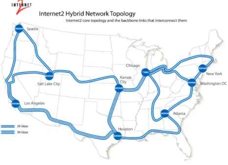
The Internet2 Network is a hybrid optical and packet network used by the U.S. research and education community. The backbone net-work consists of nine distinct routers distributed in nine different states in the U.S., as you can see in Figure 1.2.
1.3 Abilene/Internet2 Network 23 The used traces consist of the traffic related to these routers, col-lected in one week, and organized into 2016 files, each one containing data about five minutes of traffic (Netflow data). To be noted that the last 11 bits of the IP addresses are anonymized for privacy reasons; nevertheless we have more than 220000 distinct IP addresses.
Since the data provided by the Internet2 project do not have a ground truth file, we are not capable of saying a priori if any anomaly is present in the data. Because of this reason we have performed a manual verification of the data (according to the method presented in [10]), analyzing the traces for which our system reveals the biggest anomalies. Moreover we have synthetically added some anomalies in the data, so as to be able to correctly interpret the offered results. In more detail, we have added anomalies that can be associated to DoS and DDoS attacks, represented by four or five distinct traffic flows, each one carrying a traffic of 5 · 108 bytes (154 anomalies in total), that span over a single or multiple time-bins.
Since the proposed systems work with ASCII data files, in all these systems, the input data are processed by a module called, Data For-matting. This module is responsible of reading the Netflow [11] traces and of transforming them in ASCII data files, by means of the Flow-Tools [12]. The output of this module is given by text files containing on each line an IP address and the number of bytes received by that IP in the last time-bin.
Note that from the Netflow traces we can extract several other traffic descriptors. Thus, instead of considering the number of bytes received by a given IP, the system administrator can easily choose of using an-other feature, if that better allows her to detect the different attacks.
Chapter 2
Sketch data model
2.1
Sketch
2.1.1 Data streaming model
In the last years, several data models have been proposed in the lit-erature. In this section, we describe the streaming data, by using the most general model: the Turnstile Model [13].
According to this model, the input data are viewed as a stream that arrives sequentially, item by item. Let I = σ1, σ2, . . . , σn be the input
stream.
Each item σt= (it, ct) consists of a key, it∈ (1, . . . , N), and a weight,
ct. The arrival of a new data item causes the update of an underlying
function Ui[t] += ct, which represents the sum of the weights of a
given key until time t.
Given the underlying function Ui[t] for all the keys of the stream, we
can define the total sum S(t), at step t, as follows: S(t) =!
i
Ui[t] (2.1)
scenar-26 Sketch data model ios. As an example, in the context of network anomaly detection, the key can be defined using one or more fields of the packet header (IP addresses, L4 ports), or entities (like network prefixes or AS number) to achieve higher level of aggregation, while the underlying function can be the total number of bytes or packets in a flow.
2.1.2 Sketch
Sketches are powerful data structures that can be efficiently used for keeping an accurate estimate of the function U .
In general, sketches are a family of data structures that use the same underlying hashing scheme for summarizing data. They differ in how they update hash buckets and use hashed data to derive estimates. Among the different sketches, the one with the best time and space bounds is the so called count-min sketch [14].
In more detail, the sketch data structure is a two-dimensional D × W array T [l][j], where each row l (l = 1, . . . , D) is associated to a given hash function hl. These functions give an output in the interval
(1, . . . , W ) and these outputs are associated to the columns of the array. As an example, the element T [l][j] is associated to the output value j of the hash function l.
Let I = {(it, ct)} be an input stream observed during a given time
interval. When a new item arrives, the sketch is updated as follows:
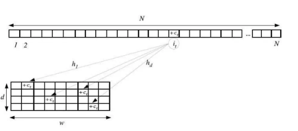
T [l][hl(it)] ← T [l][hl(it)] + ct (2.2)
The update procedure is realized for all the different hash functions as shown in Figure 2.1. In this way, at a given time-bin t, the bucket T [l][hl(it)] will contain an estimate of the quantity Ui[t].
2.1 Sketch 27
Figure 2.1: Sketch - Update Function
In this work, the sketches have been taken into consideration for two distinct reasons, which will be clearer in the following: on one hand they allow the storing of big quantities of data (in our case we have to store the traffic generated by more than 220000 IP addresses) with big memory savings, on the other hand they permit a random aggre-gation of the traffic flows. Indeed , given the use of hash functions, it is possible to have some collisions in the sketch table. In more detail, this last fact implies that each traffic flow will be part of several ran-dom aggregates, each of which will be analyzed to check if it presents any anomaly. This means that, in practice, any flow will be checked more than once (within different aggregates), thus, it will be easier to detect an anomaly. Indeed an anomaly could be masked in a given traffic aggregate, while being detectable in another one.
28 Sketch data model
2.1.3 Reversible Sketch
Sketch data structures have a major drawback: they are not reversible. That is, a sketch cannot efficiently report the set of all keys (in our case, the flows) that correspond to a given bucket.
To overcome such a limitation, [15] proposes a novel algorithm for efficiently reversing sketches.
The basic idea is to perform an “intelligent” hash by modifying the input keys and/or the hashing functions so as to make possible to recover the keys with certain properties like big changes without sac-rificing the detection accuracy.
In more detail the update procedure for the k-ary sketch is modified by introducing modular hashing and IP mangling techniques.
The modular hashing works partitioning the n-bit long hash key x into q words of equal length n/q, that are hashed separately using a different hash function, hdi (i = (1, . . . , q)) (let us consider that
the output of each function is m-bit long). Finally, these outputs are concatenated to form the final hash value (as depicted in Figure 2.2).
δd(x) = hd1(x)|hd2(x)| . . . |hdq(x) (2.3)
Since the final hash value consists of q × m bits, it can assume w = 2q×m different values.
Note that the use of the modular hashing can cause a highly skewed distribution of the hash outputs. Consider, as an example, our case in which IP addresses are used as hash keys. In network traffic streams there are strong spatial localities in the IP addresses since many IP addresses share the same prefix. This means that the first octets
2.1 Sketch 29
Figure 2.2: Modular Hashing
(equal in most addresses) will be mapped into the same hash values increasing the collision probability of such addresses.
To effectively resolve this problem, the IP mangling technique has to be applied before computing the hash functions. By using such a technique the system randomizes, in a reversible way, the input data so as to remove the correlation or spatial locality.
Essentially, this technique transforms the input set to a mangled set and performs all the operations on this set. The output is then transformed back to the original input keys. The function used for such a transformation is a bijective (one-to-one) function from key space [2n] to [2n].
A typical function used for this purpose is a function of the form
f (x) ≡ a· x mod 2n (2.4)
with a and 2n relatively prime to guarantee the invertibility of the
30 Sketch data model The mangled key can easily be reversed by computing a−1 and
ap-plying the same function to the mangled key, using a−1 instead of a.
This function has the advantage of being extremely fast to compute but performs well only for non-adversarial key spaces in which no cor-relation exists among keys that have different (non empty) prefixes. Indeed, for any two keys that share the last bits, the mangled ver-sions will also share the same last bits. Thus distinct keys that have common suffixes will be more likely to collide than keys with distinct suffixes.
However, in the particular case of IP addresses, this is not a prob-lem. Due to the hierarchical nature of IP addresses, it is perfectly reasonable to assume that there is no correlation between the traffic of two IP addresses if they differ in their most significant bits.
However, this is not a safe assumption in general. For example, in the case of keys consisting of source and destination IP address pairs, the hierarchical assumption should not apply, and we expect to see traffic correlation among keys sharing the same destination IP but completely different IP source. And even for single IP address keys, it is plausible that an attacker could antagonistically cause a non-heavy-change IP address to be reported as a false positive by creating large traffic changes for an IP address that has a similar suffix to the target - also known as behavior aliasing.
Thus, to prevent adversarial attacks against the hashing scheme, a more sophisticated mangling function is needed.
In [15] the authors propose an attack-resilient scheme based on sim-ple arithmetic operations on a Galois Extension Field GF(2l), where
2.1 Sketch 31 l = log22n.
The function is now defined as follows:
f (x) ≡ a ⊗ x ⊕ b (2.5)
where “ ⊗ ” is the multiplication operation defined on GF(2l) and “ ⊕ ” is the bit-wise XOR operation. a and b are randomly chosen from {1, 2, · · · , 2l− 1}.
By precomputing a−1 on GF(2l), we can easily reverse a mangled key y using
f−1(y) = a−1⊗ (x ⊕ b). (2.6)
The direct computation of a ⊗ x can be very expensive, as it would require multiplying two polynomials (of degree l − 1) modulo an irre-ducible polynomial (of degree l) on a Galois Field GF(2).
In practice this mangling scheme effectively resolves the highly skewed distribution caused by the modular hash functions as shown in Figure 2.3. Figure 2.3 shows the distribution of the number of keys (source IP address of each flow) per bucket for three different hashing scheme:
• modular hashing with no IP mangling
• modular hashing with the GF transformation for IP mangling • direct hashing (a completely random hash function)
We observe that the key distribution of modular hashing with the GF transformation is essentially the same as that of direct hashing. The distribution for modular hashing without IP mangling is highly skewed.
32 Sketch data model
Figure 2.3: IP Mangling - Distribution of number of keys for each bucket
Thus IP mangling is very effective in randomizing the input keys and removing hierarchical correlations among the keys. In addition, the scheme is resilient to behavior aliasing attacks because attackers cannot create collisions in the reversible sketch buckets to make up false positive heavy changes. Any distinct pair of keys will be mapped completely randomly to two buckets for each hash table.
The other key point introduced in [15] is the algorithm for reversing the sketch, given the use of modular hashing and IP mangling.
2.1 Sketch 33 Notation for the general algorithm
Let us introduce some notations useful for understanding the algo-rithm.
Let the dth row of the sketch table contain td heavy buckets. Let t
be the value of the largest td. For each row of the sketch assign an
arbitrary indexing of the tdheavy buckets and let td,j be the index in
the row d of heavy bucket number j. Also define σp(x) to be the pth
word of a q word integer x. For example, if the jth heavy bucket in the row d is td,j = 5.3.0.2 for q = 4, then σ2(td,j) = 3.
For each d ∈ [D] and word p, denote the reverse mapping set of each modular hash function hd,p by the 2m× 2
n
q−m table h−1
d,w of nq bit
words. That is, let h−1d,w[j][k] denote the kth 2nq bit key in the reverse
mapping of j for hd,p. Further, let h−1d,p[j] = {x ∈ [2
n q]|h
d,p(x) = j}.
Let Ip = {x|x ∈"tj=0d−1h−1d,w[σp(td,j)] for at least D−r values d ∈ [D]}.
That is, Ip is the set of all x ∈ [2
n
q] such that x is in the reverse
mapping for hd,pfor some heavy bucket in at least D −r of the D hash
tables. We occasionally refer to this set as the intersected modular potentials for word p. For instance, in Figure 2.4, I1has three elements
and I2 two.
For each word we also define the mapping Bp which specifies for
any x ∈ Ip exactly which heavy buckets x occurs in for each hash
table. In detail, Bp(x) = (Lp[0][x], Lp[1][x], . . . , Lp[D − 1][x]) where
Lp[i][x] = {j ∈ [t]|x ∈ h−1d,p[σp(ti,j)]}"∗. That is, Lp[i][x] denotes the
collection of indices in [t] such that x is in the modular bucket potential set for the heavy bucket corresponding to the given index. The special character ∗ is included so that no intersection of sets Lp yields an
34 Sketch data model means that the reverse mapping of the 1st , 3rd , and 8th heavy bucket under h0,p all contain the modular key 129.
We can think of each vector Bp(x) as a set of all D dimensional
vectors such that the dth entry is an element of Lp[d][x]. For
exam-ple, B3(23) = ({1, 3}, {16}, {∗}, {9}, {2}) is indeed a set of two
vec-tors: ({1}, {16}, {∗}, {9}, {2}) and ({3}, {16}, {∗}, {9}, {2}. We refer to Bp(x) as the bucket index matrix for x, and a decomposed vector
in a set Bp(x) as a bucket index vector for x. We note that although
the size of the bucket index vector set is exponential in D, the bucket index matrix representation is only polynomial in size and permits the operation of intersection to be performed in polynomial time. Such a set like B1(a) can be viewed as a node in Figure 2.4.
Define the r intersection of two such sets to be B#rC = {v ∈ B#C|v has at most r of its D entries equal to ∗}. For example, Bp(x)#rBp+1(y) represents all of the different ways to choose a
sin-gle heavy bucket from each of at least D − r of the hash tables such that each chosen bucket contains x in its reverse mapping for the pth word and y for the p + 1th word. For instance, in Figure 2.4, B1(a)#rB2(d) = ({2}, {1}, {4}, {∗}, {3}), which is denoted as a link
in the figure. Note that there is not such a link between B1(a) and
B2(e). Intuitively, the a.d sequence can be part of a heavy change key
because these keys share common heavy buckets for at least D − r hash tables. In addition, it is clear that a key x ∈ [2n] is a suspect
key for the sketch if and only if#rp=1...qBp(xp) += 0.
Finally, we define the sets Ap which we compute in our algorithm
to find the suspect keys. Let A1= {((x1), v)|x1 ∈ I1and v ∈ B1(x1)}.
2.1 Sketch 35 Aw and v ∈ Bw+1(xw+1)}. Take Figure 2.4 for example. Here A4
con-tains (a, d, f, i), (2, 1, 4, ∗, 3) which is the suspect key. Each element of Ap can be denoted as a path in Figure 2.4. The following lemma
tells us that it is sufficient to compute Aq to solve the reverse sketch
problem.
Lemma 1 A key x = x1· x2. . . xq ∈ [2n] is a suspect key if and only
if ((x1, x2, . . . , xq), v) ∈ Aq for some vector v.
General algorithm for Reverse Hashing
To solve the reverse sketch problem we first compute the q sets Ip and
bucket index matrices Bp. From these we iteratively create each Ap
starting from some base Ac for any c where 1 ≤ c ≤ q up until we
have Aq. We then output the set of heavy change keys via Lemma
1. Intuitively, we start with nodes as in Figure 2.4, I1 is essentially
A1. The links between I1 and I2 give A2, then the link pairs between
(I1I2) and (I2I3) give A3, etc.
The choice of the base case Ac affects the performance of the
algo-rithm. The size of the set A1 is likely to be exponentially large in
D. However, with good random hashing, the size of Ap for p ≥ 2
will be only polynomial in D, q, and t with high probability with the detailed algorithm and analysis below. Note we must choose a fairly small value c to start with because the complexity of computing the base case grows exponentially in c.
The pseudocode of the Reverse Hashing algorithm is reported in Algorithm 1. Instead, the pseudocode for the functions M ODU LAR P OT EN T IALS and EXT EN D is reported in Algorithms 2 and 3, respectively.
36 Sketch data model Algorithm 1 REVERSE HASH(r)
1: for p = 1 : l do
2: (IpBp) = M ODU LAR P OT EN T IALS(p, r)
3: end for 4: A2 = 0
5: for x ∈ I1, y ∈ I2 and corresponding v ∈ B1(x)#rB2(y) do
6: insert ((x, y), v) into A2
7: end for
8: for any given Ap do
9: Ap+1= EXT EN D(Ap, Ip+1, Bp+1)
10: end for
11: Output all x1.x2. · · · .xq ∈ [n] s.t. ((x1, . . . , xq), v) ∈ Aq for some
v
2.2
Implementation
Reversible Sketches are a common substrate for all the proposed sys-tems, used to perform a random aggregation of the data.
In the implemented systems, the module responsible for the con-struction of the reversible sketch tables takes in input the data files described in Section 1.2.
As said before, each line of these files contains an IP destination address and the number of the bytes received by that IP in the last time bin (i.e. five minutes of traffic).
Each file is thus used to build a distinct sketch table. In more detail, according to the Tunstile model, presented in Section 2.1.1, the IP address IPt is considered as the hash key it, while the number of
2.2 Implementation 37 Algorithm 2 MODULAR POTENTIALS(p, r)
1: Create an D × 2
n
q table of sets L initialized to all contain the
special character ∗
2: Create a size [2nq] array of counters hits initialized to all zeros
3: for i ∈ [D], j ∈ [t], and k ∈ [2 n q−m] do 4: insert h−1d,p[σp(td,j)][k] into L[d][x] 5: if L[d][x] == 0 then 6: hits[x] + + 7: end if 8: end for 9: for x ∈ [2 n q] s.t. hits[x] ≥ D − r do 10: insert x into Ip 11: Bp(x) = (L[0][x], L[1][x], . . . L[D − 1][x]) 12: end for 13: Output (Ip, Bp) Algorithm 3 EXTEND(Ap, Ip+1, Bp+1) 1: Ap+1= 0 2: for y ∈ Ip+1, ((x1, . . . , xp), v) ∈ Ap do
3: if thenv#rBp+1(y) += null)
4: insert ((x1, . . . , xp), v#rBp+1(y)) into Ap+1
5: end if 6: end for 7: Output (Ap+1)
Note that in our implementation we have used d = 32 distinct hash functions, which give output in the interval [0; w −1], that means that
38 Sketch data model the resulting sketches will be ∈ Nd×w, where w can be varied.
As far as the hash functions are concerned, we have used 4-universal hashes1 [16], obtained as:
h(x) =
3
!
i=0
ai· xi mod p mod w (2.7)
where the coefficients ai are randomly chosen in the set [0, p − 1] and
p is an arbitrary prime number (we have considered the Mersenne numbers).
At this point, given that we had N distinct time-bins, we have ob-tained N distinct sketch tables. Starting from these we consider the temporal evolution of each bucket Tlj of the sketch table, constructing
d · w time series of N samples Tlj[n] each.
The pseudocode about the sketch computation is given in Algorithm 4.
For sake of brevity we do not describe the function IP M AN GLIN G and M ODU LAR HASHIN G already described in Section 2.1.3.
1
A class of hash functions H : (1, . . . , N ) → (1, . . . , w) is a k-universal hash if for any distinct x0, . . . xk−1∈ (1, . . . , N ) and any possible v0, . . . vk−1∈ (1, . . . , w):
2.2 Implementation 39
Algorithm 4 Building the sketch
1: Input: IP destination address - ip1.ip2.ip3.ip4
2: for l = 1 : d do 3: forj = 1 : w do
4: Tn[l][j] = 0 ! sketch table initialization
5: end for 6: end for
7: for n = 1 : N do 8: fort = 1 : S do
9: IP M AN GLIN G(ipt)
10: δ = M ODU LAR HASHIN G(ipt)
11: Store : ip1t, ip2t, ip3t, ip4t 12: forl = 1 : d do 13: Tn[l][δ]+ = Bt 14: end for 15: end for 16: end for
40 Sketch data model
Chapter 3
Principal Component
Analysis
3.1
Pricipal Component Analysis
The Principal Components Analysis (PCA) is a linear transformation that maps a coordinate space onto a new coordinate system whose axes, called Principal Components (PCs), have the property to point in the direction of maximum variance of the residual data (i.e., the difference between the original data and the data mapped onto the previous PCs).
In more detail, the first PC captures the greatest degree of data variance in a single direction, the second one captures the greatest degree of variance of data in the remaining orthogonal directions, and so on.
A simple illustration of the PCA is shown in Figure 3.1 where the PCs of a two dimensional dataset are plotted. As you can see in the figure, the number of PCs is equal to the dimensionality of the original dataset; the first PC is in the direction that maximizes the variance of the projected data (green line), the second PC, instead, is in the
42 Principal Component Analysis orthogonal direction (blue line).
Figure 3.1: PCs of a two-dimentional dataset
In mathematical terms, to calculate the PCs is equivalent to compute the eigenvectors of the covariance matrix.
In more detail, given the matrix of data B = {Bi,j}, with 1 < i < m
and 1 < j < t (e.g., a dataset of m samples captured in t time-bins), each PC, vi, is the i − th eigenvector computed from the spectral
decomposition of the covariance matrix C = BBT, that is:
BBTv
i = λivi i = 1, . . . , m (3.1)
where λi is the “ordered” eigenvalue corresponding to the eigenvector
vi.
3.1 Pricipal Component Analysis 43
v1= arg max #v#=1 .Bv.
(3.2)
where .Bv.2 is proportional to the variance of the data measured
along v.
Proceeding recursively, once the first k−1 PCs have been determined, the k − th PC can be evaluated as follows:
vk= arg max #v#=1 $ $ $ $ $(B − k−1 ! i=1 BviviT)v $ $ $ $ $ (3.3)
where || · || denotes the L2 norm.
Once the PCs have been computed, given a set of data and its as-sociated coordinate space, we can perform a data transformation by projecting them onto the new axis.
Typically, the first PCs contribute most of the variance in the original dataset, so that we can describe them with only these PCs, neglecting the others, with minimal loss of variance.
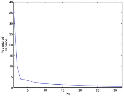
For this reason, the PCA is also used as a linear dimension reduction technique. The main idea is to calculate the PCs and establish how many of them are sufficient to describe the original dataset. To select the PCs we can perform the scree plot method.
A scree-plot is a plot, like the one represented in Figure 3.2, of the percentage of variance captured by a given PC. Thus, studying the scree plot we can determine the optimal number of variables, in order to lower the dimensionality of a complex dataset, while maintaing the most of the variance of the original dataset.
44 Principal Component Analysis 5 10 15 20 25 30 0 5 10 15 20 25 30 35 40 PC % captured variance
Figure 3.2: Scree Plot
3.2
System architecture
In this Section, we present the architecture of the system we have implemented to detect anomalies in the network traffic.
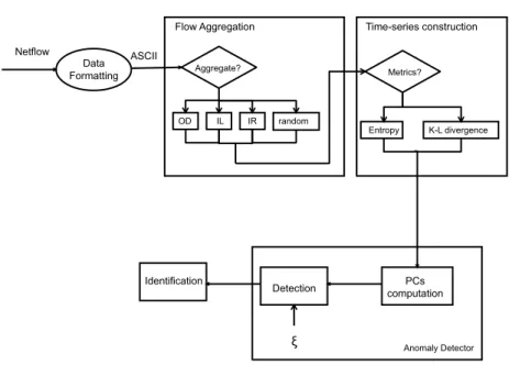
In Figure 4.3 is reported a block scheme of the proposed system. We can distinguish four main block:
• Data Formatting • Flow Aggregation
• Time-series Construction • Anomaly Detector
3.2 System architecture 45 • Identification
Figure 3.3: PCA - System Architecture
For sake of brevity we skip the detail related to the Data Formatting module since a detailed analysis of this block has been made in Section 1.2.
3.2.1 Flow Aggregation
To facilitate the detection of correlation and periodic trends in the data, we have studied different levels of aggregation. In more de-tail, the block called Flow Aggregation realizes four different levels of aggregation:
46 Principal Component Analysis • Ingress Router (IR)
• Origin Destination (OD) flows • Input Link (IL)
• Random Aggregation
Using the IR aggregation, data are organized according to which router they entered the network. The OD flow aggregates traffic based on the ingress and egress routers used by an IP flow. Instead, the IL aggregates IP flows with the same ingress router and input interface. Finally, the random aggregation is performed by means of the sketch (as described in Chapter 2).
The output of this block is given by 4T distinct files, each one cor-responding to a specific time-bin and a specific aggregate.
3.2.2 Time-series Construction
After the data have been correctly formatted, they are passed as input to the third module, responsible for the construction of the time-series. Typically the distribution of packet features (packet header fields) observed in flow traces reveals both the presence and the “structure” of a wide range of anomalies. Indeed, traffic anomalies induce changes in the normal distribution of the features.
Based on this observation, we have examined the distributions of traffic features as a means to detect and to classify network anomalies. More specifically, in this work, we have taken into consideration the number of bytes sent by each IP source address.
3.2 System architecture 47 The feature distribution has been estimated with the empirical his-togram. Thus, in each time-bin for each aggregate we have evaluated the histogram as follows:
Xt= {nti, i = 1, . . . , N } (3.4)
where nt
i is the number of bytes transmitted by the i − th IP address
in the time-bin t.
Unfortunately, the histogram is an high-dimensional object quite difficult to handle with low computational resources.
For this reason we have tried to concentrate the information taken by the histogram in a single value, able to hold the most of the useful information, that, in our case, is the trend of the distribution.
Previous works [17] [18] [10] have emphasized the possibility to ex-tract very useful information from the entropy of the distribution.
The entropy provides a computationally efficient metric for estimat-ing the degree of dispersion or concentration of a distribution.
Given the empirical histogram, Xt, we can evaluate the entropy value
as follows: Ht= − N ! i=1 nt i S log2 nt i S with S = N ! i=1 nt i (3.5)
Nevertheless, the entropy is only able to capture the information related to a single time-bin, while from our point of view it would be much more important to capture the the difference between packet feature distributions of two adjacent time-bins.
For this reason, in this work we have also used another metric that is the Kullback-Leibler (KL) divergence. Given two histograms Xt
48 Principal Component Analysis (captured in time-bin t) and Xt−1 (captured in time-bin t − 1), the
KL divergence is defined as follows:
DtKL= N ! i=1 nt−1i logn t−1 i nt i (3.6) Despite of the method used, this module will output a matrix for each type of aggregation in which, for all the aggregates, the values of the metric (entropy or KL divergence) evaluated in each time-bin are reported.
This matrix has the following structure:
Y = y11 · · · y1N .. . ... yT1 · · · yT N (3.7)
where N is the number of aggregates and T the number of time-bins.
3.2.3 Anomaly Detector
This block is the main component of the detection system. It consists of a Detection phase, during which the system detects anomalies by means of the PCA technique, and an Identification phase to identify the IPs responsible of the anomalies.
PCs computation
After the time-series have been constructed, they are passed to the module that applies the PCA. The computation of the PCs is per-formed using Equations (3.2) and (3.3). As described before, typically
3.2 System architecture 49 there is a set of PCs (called dominant PCs) that contributes most of the variance in the original dataset.
The idea is to select the dominant PCs and describe the normal behavior only using these ones.
It is worth highlighting that the number of dominant PCs is a very important parameter, and needs to be properly tuned when using the PCA as a traffic anomaly detector.
In our approach the set of dominant PCs is selected by means of the scree-plot method. As a result, we separate the PCs into two sets, dominant and negligible PCs, that will be then used to distinguish between normal and anomalous variations in traffic.
Figure 3.2 reports a scree-plot of a particular dataset used in our study. Visually, from the graph we can observe that the first r = 5 PCs are able to correctly capture the majority of the variance. These PCs are the dominant PCs:
P = (v1, . . . , vr) (3.8)
The method is based on the assumption that these PCs are sufficient to describe the normal behavior of traffic.
Detection Phase
The detection phase is performed by separating the high-dimensional space of traffic measurements into two subspaces, which capture nor-mal and anonor-malous variations, respectively.
In more detail, once the matrix P has been constructed, we can par-tition the space into a normal subspace ( ˆS), spanned by the dominant PCs, and an anomalous subspace ( ˜S), spanned by the remaining PCs
50 Principal Component Analysis The normal and anomalous components of data can be obtained by projecting the aggregate traffic onto these two subspaces.
Thus, the original data, in the time-bin t, Yt are decomposed into
two parts as follows:
Yt= ˆYt+ ˜Yt (3.9)
where ˆYt and ˜Yt are the projection onto ˆS and ˜S, respectively, and
can be evaluate as follows:
ˆ
Yt= P PTYt (3.10)
˜
Yt= (I − P PT)Yt (3.11)
To be noted that, when anomalous traffic crosses the network, a large change in the anomalous component ( ˜Yt) occurs. Thus, an efficient
method to detect traffic anomalies is to compare . ˜Yt.2 with a given
threshold (ξ).
In more detail, if . ˜Yt.2 exceeds the given threshold ξ, the traffic is
considered anomalous, and we mark the time-bin (t) as an anomalous time-bin (Figure 3.4).
If we use a random aggregation the detection phase can be improved performing a further step.
Indeed, in this case, since we have used d different hash functions hj
we have d data matrices, Yj (one for each function). So, the
previ-ously described analysis (performed for each Yj) returns d different
3.2 System architecture 51
Figure 3.4: PCA - Data matrix
Thus, a voting analysis is performed. We evaluate the number of produced alarms and we decide if the time-bin is anomalous or not according to the following rule:
anomalous if number of alarms > d 2− 1
normal otherwise
More details about the detection phase are given in Algorithm 5.
3.2.4 Identification
If an anomaly has been detected, the system performs a further phase called anomaly identification.
Note that the PCA works on a single time-series, so in the detec-tion phase we are able to identify the time-bin during which traffic is anomalous. But, at this point, we do not know the specific network event that has caused the detection.
52 Principal Component Analysis Algorithm 5 Detection
1: Input: Data matrices - Yj, j = 0, . . . , d
2: alarm = 0 3: for j = 1 : d do 4: Compute the P Cs
5: Select the dominant P Cs : P = (v1, . . . , vr)
6: Y˜j= (I − P PT)Yj ! anomalous component of the traffic
7: if % ˜Yt% 2 > ξ then 8: alarm + + 9: end if 10: end for 11: if alarm >d 2 − 1 then
12: the time-bin is anomalous 13: end if
In fact, it is worth noticing that an anomalous time-bin may contain multiple anomalous events, and that a single anomalous event can span over multiple time-bins.
In this phase we want to identify the specific flows responsible for the revealed anomaly.
Note that if the traffic aggregation is performed by means of IR, OD flow, and IL we are not able to determine the specific flow responsible for the revealed anomaly.
On the contrary, when we use random traffic aggregation, since we use the reversible sketches, we are able to correctly identify the spe-cific flows involved in the anomalous traffic. In more detail, at first, we search the specific traffic aggregation in which the anomaly has occurred. Then reversing the sketch we can identify the specific flows that have caused the anomaly.