A computational fluid-dynamic study of the three-dimensional flow in the stator of a gas turbine stage with hot streak injection

(1)

Politecnico di Milano

School of Industrial and Information Engineering

Master of Science in Mechanical Engineering

A computational fluid-dynamic study of the

three-dimensional flow in the stator of a gas

turbine stage with hot streak injection

Supervisor: Prof. Giacomo Bruno Azzurro PERSICO

Candidate:

Ivano Sammarco Matr. 905549

(2)

(3)

Abstract

This work presents the results of a numerical study about the migration and evolution of hot streaks generated by combustor burners, during their transport through the first stage of an un-cooled turbine. The hot streaks are injected at 70% of the span in the streamwise direction at the inlet of the stage in four circumferential positions with respect to the stator blade. The hot streaks are controlled in order to provide an over-value to the distribution of temperature of approximately 20% with respect to the main flow. The numerical results achieved through the commercial code ANSYS-CFX are progressively compared with mea-surements performed in the high-speed closed-loop test rig of the Laboratorio di Fluidodinamica delle Macchine (LFM) of the Politecnico di Milano. The aim of this study is to investigate and provide interpretation of the experimental results that mainly show a severe temperature attenuation of the hot streaks within the stator cascade highly dependent on the injection azimuthal position. Simulations exhibit a good agreement with experiments on the measurements planes and allow to better understand the complex flow phenomena occurring between the blade rows.

(4)

(5)

List of Figures

1.1 (A) Meridional cut of the test section; T0=stator upstream traverse; T1=stator downstram; T2=rotor downstream; HSG, hot streak generator; HP, high pressure stage; (B) Injector to stator vane

position for the pressure side case test point . . . 3

1.2 Turbine chasing isometric view . . . 4

1.3 Internal view of channel with an EWG injector upstream of the stator 4 1.4 Different blade geometries: cylindrical, leaned and bowed. . . 5

1.5 Isobars distribution. . . 6

1.6 Lean effect on the distribution of the secondary flows. . . 7

1.7 Hub clearance at the hub trailing edge of the stator. . . 7

1.8 Description of a passage vortex given by a non-uniform inlet velocity profile along the blade height. . . 8

1.9 Sheet vortexes at the stage outlet. . . 9

1.10 Interaction between horse-shoe and passage vortexes. . . 10

1.11 Interaction between passage, leakage and scraping vortexes for compressor and turbine blades. . . 11

1.12 Absolute flow angle downstream of the stage for the different oper-ating conditions. . . 13

2.1 Temperature ratio between the core of the hot streak and the main stream (A), and total pressure (B) fields of the hot streak. Pmean is reported as a difference between the local total pressure and the main stream pressure (kinetic head = 1100Pa). (C) RMS of the total pressure. . . 15

2.2 Total temperature fields downstream of the stator for the four hot streak positions. . . 17

2.3 Streamwise vorticity for (A) MP injection, (B) PS injection, (C) SS injection. . . 18

3.1 Computational domain. . . 19

3.2 Inlet total pressure (A) and outlet static pressure (B) boundary conditions in OP3. . . 20

(8)

LIST OF FIGURES

3.3 Inlet total pressure (A) and outlet static pressure (B) boundary conditions in OP1. . . 21 3.4 Inlet total temperature (A) and total pressure (B) boundary

condi-tions in OP3 with hot streak injection. . . 21 3.5 Inlet turbulence intensity boundary condition in OP3 with hot

streak injection. . . 22 3.6 Eddy length scale boundary condition in OP3 with hot streak injection. 23 4.1 Inlet view of blade wall mesh (A) and zoomed frame of the hub

region (B) with no clearance. . . 26 4.2 Total pressure loss coefficient circumferential average in spanwise

direction in OP3 reference condition for mesh with no clearance. . 27 4.3 Mach number circumferential average in spanwise direction in OP3

reference condition for mesh with no clearance. . . 28 4.4 Static pressure circumferential average in spanwise direction in OP3

reference condition for mesh with no clearance. . . 28 4.5 Total pressure circumferential average in spanwise direction in OP3

reference condition for mesh with no clearance. . . 29 4.6 Comparison of the total pressure loss coefficient between (A)

exper-iments and (B) computational results on the measurement plane at the exit of the stator in OP3 reference condition for mesh with no clearance. . . 30 4.7 Comparison of the static pressure loss coefficient between (A)

ex-periments and (B) computational results on the measurement plane at the exit of the stator in OP3 reference condition for mesh with no clearance. . . 31 4.8 Comparison of the Mach number between (A) experiments and (B)

computational results on the measurement plane at the exit of the stator in OP3 reference condition for mesh with no clearance. . . 31 4.9 Comparison of the streamwise vorticity between (A) experiments

and (B) computational results on the measurement plane at the exit of the stator in OP3 reference condition for mesh with no clearance. 32 4.10 Total pressure loss coefficient circumferential average in spanwise

direction in OP1 reference condition for mesh with no clearance. . 33 4.11 Mach number circumferential average in spanwise direction in OP1

reference condition for mesh with no clearance. . . 34 4.12 Static pressure circumferential average in spanwise direction in OP1

reference condition for mesh with no clearance. . . 34 4.13 Total pressure circumferential average in spanwise direction in OP1

reference condition for mesh with no clearance. . . 35 VI

(9)

LIST OF FIGURES

4.14 Comparison of the total pressure loss coefficient between (A) exper-iments and (B) computational results on the measurement plane at the exit of the stator in OP1 reference condition for mesh with no clearance. . . 36 4.15 Comparison of the static pressure between (A) experiments and (B)

computational results on the measurement plane at the exit of the stator in OP1 reference condition for mesh with no clearance. . . 36 4.16 Comparison of the Mach number between (A) experiments and (B)

computational results on the measurement plane at the exit of the stator in OP1 reference condition for mesh with no clearance. . . 37 4.17 Comparison of the streamwise vorticity between (A) experiments

and (B) computational results on the measurement plane at the exit of the stator in OP1 reference condition for mesh with no clearance. 37 4.18 Inlet view of blade wall mesh (A) and zoomed frame of the hub

region (B) with the clearance at the hub trailing edge. . . 38 4.19 Total pressure loss coefficient circumferential average in spanwise

direction in OP3 reference condition for mesh with clearance at the hub of the blade. . . 39 4.20 Total pressure circumferential average in spanwise direction in OP3

reference condition for mesh with clearance at the hub of the blade. 40 4.21 Mach number circumferential average in spanwise direction in OP3

reference condition for mesh with clearance at the hub of the blade. 40 4.22 Static pressure circumferential average in spanwise direction in OP3

reference condition for mesh with clearance at the hub of the blade. 41 4.23 Comparison of the total pressure loss coefficient between (A)

exper-iments and (B) computational results on the measurement plane at the exit of the stator in OP3 reference condition for mesh with clearance. . . 41 4.24 Comparison of the static pressure between (A) experiments and (B)

computational results on the measurement plane at the exit of the stator in OP3 reference condition for mesh with clearance. . . 42 4.25 Comparison of the Mach number between (A) experiments and (B)

computational results on the measurement plane at the exit of the stator in OP3 reference condition for mesh with clearance. . . 42 4.26 Comparison of the streamwise vorticity between (A) experiments

and (B) computational results on the measurement plane at the exit of the stator in OP3 reference condition for mesh with clearance. 43 4.27 Total pressure loss coefficient circumferential average in spanwise

direction in OP1 reference condition for mesh with clearance at the hub of the blade. . . 44 4.28 Total pressure circumferential average in spanwise direction in OP1

(10)

LIST OF FIGURES

4.29 Mach number circumferential average in spanwise direction in OP1 reference condition for mesh with clearance at the hub of the blade. 45 4.30 Static pressure circumferential average in spanwise direction in OP1

reference condition for mesh with clearance at the hub of the blade. 45 4.31 Comparison of the total pressure loss coefficient between (A)

exper-iments and (B) computational results on the measurement plane at the exit of the stator in OP1 reference condition for mesh with clearance. . . 46 4.32 Comparison of the static pressure between (A) experiments and (B)

computational results on the measurement plane at the exit of the stator in OP1 reference condition for mesh with clearance. . . 46 4.33 Comparison of the Mach number between (A) experiments and (B)

computational results on the measurement plane at the exit of the stator in OP1 reference condition for mesh with clearance. . . 47 4.34 Comparison of the streamwise vorticity between (A) experiments

and (B) computational results on the measurement plane at the exit of the stator in OP1 reference condition for mesh with clearance. 47 4.35 Inlet view of blade wall mesh (A) and zoomed frame of the hub

region (B) with the gap all along the hub of the blade. . . 48 4.36 Total pressure loss coefficient circumferential average in spanwise

direction in OP3 reference condition for mesh with gap all along the hub of the blade. . . 49 4.37 Total pressure circumferential average in spanwise direction in OP3

reference condition for mesh with gap all along the hub of the blade. 50 4.38 Mach number circumferential average in spanwise direction in OP3

reference condition for mesh with gap all along the hub of the blade. 50 4.39 Static pressure circumferential average in spanwise direction in OP3

reference condition for mesh with gap all along the hub of the blade. 51 4.40 Comparison of the total pressure loss coefficient between (A)

exper-iments and (B) computational results on the measurement plane at the exit of the stator in OP3 reference condition for mesh with 0.5mm gap all along the hub. . . 51 4.41 Comparison of the static pressure between (A) experiments and

(B) computational results on the measurement plane at the exit of the stator in OP3 reference condition for mesh with 0.5mm gap all along the hub. . . 52 4.42 Comparison of the Mach number between (A) experiments and (B)

computational results on the measurement plane at the exit of the stator in OP3 reference condition for mesh with 0.5mm gap all along the hub. . . 52

(11)

LIST OF FIGURES

4.43 Comparison of the streamwise vorticity between (A) experiments and (B) computational results on the measurement plane at the exit of the stator in OP3 reference condition for mesh with 0.5mm gap all along the hub. . . 53 4.44 Three-dimensional view of the selected planes for the representation

of the vorticity evolution throughout the domain. . . 54 4.45 Streamwise vorticity represented on selected secondary planes

through-out the domain with the 0.5mm gap in OP3 reference condition. . 55 4.46 Total pressure loss coefficient circumferential average in spanwise

direction in OP1 reference condition for mesh with gap all along the hub of the blade. . . 56 4.47 Total pressure circumferential average in spanwise direction in OP1

reference condition for mesh with gap all along the hub of the blade. 56 4.48 Mach number circumferential average in spanwise direction in OP1

reference condition for mesh with gap all along the hub of the blade. 57 4.49 Static pressure circumferential average in spanwise direction in OP1

reference condition for mesh with gap all along the hub of the blade. 57 4.50 Comparison of the total pressure loss coefficient between (A)

exper-iments and (B) computational results on the measurement plane at the exit of the stator in OP1 reference condition for mesh with 0.5mm gap all along the hub. . . 58 4.51 Comparison of the static pressure between (A) experiments and

(B) computational results on the measurement plane at the exit of the stator in OP1 reference condition for mesh with 0.5mm gap all along the hub. . . 58 4.52 Comparison of the Mach number between (A) experiments and (B)

computational results on the measurement plane at the exit of the stator in OP1 reference condition for mesh with 0.5mm gap all along the hub. . . 59 4.53 Comparison of the streamwise vorticity between (A) experiments

and (B) computational results on the measurement plane at the exit of the stator in OP1 reference condition for mesh with 0.5mm gap all along the hub. . . 59 4.54 Comparison between OP3 and OP1 reference conditions of (A) Mach

number, (B) blade loading, (C) absolute flow angle and (D) total pressure loss coefficient distributions. . . 60 4.55 Comparison between computational (left column) and experimental

(right column) streamwise vorticity at the stator exit for (A) OP3 and (B) OP1 operative conditions. . . 62 5.1 Computational domain. . . 63

(12)

LIST OF FIGURES

5.2 Comparison of the total temperature (A) and total pressure loss coefficient (B) between experimental campaign and computational results for k-ε, SST k-ω and BSL-RSM turbulence models with LE injection. . . 64 5.3 Comparison of the total temperature (A) and total pressure loss

coefficient (B) between experimental campaign and computational results for k-ε, SST k-ω and BSL-RSM turbulence models with MP injection. . . 65 5.4 Comparison of the total temperature (A) and total pressure loss

coefficient (B) between experimental campaign and computational results for k-ε, SST k-ω and BSL-RSM turbulence models with PS injection. . . 66 5.5 Comparison of the total temperature (A) and total pressure loss

coefficient (B) between experimental campaign and computational results for k-ε, SST k-ω and BSL-RSM turbulence models with SS injection. . . 67 5.6 Comparison of the total temperature between (A) experiments and

(B) computational results on the measurement plane at the exit of the stator for leading edge (LE) injection case. . . 68 5.7 Comparison between computational (left column) and experimental

(right column) streamwise vorticity at the stator exit for LE case: (A) with injection; (B) with no injection. . . 69 5.8 Comparison between computational (left column) and experimental

(right column) total pressure loss coefficient at the stator exit for LE case: (A) with injection; (B) with no injection; (C) point-to-point Y difference (hot streak−no injection). . . 70 5.9 Comparison between computational (left column) and experimental

(right column) results for the LE injection: (A) total pressure loss coefficient and (B) absolute flow angle spanwise profiles. . . 71 5.10 Comparison of the total temperature between (A) experiments and

(B) computational results on the measurement plane at the exit of the stator for mid-pitch (MP) injection case. . . 72 5.11 Comparison between computational (left column) and experimental

(right column) total pressure loss coefficient at the stator exit for MP case: (A) with injection; (B) with no injection; (C) point-to-point Y difference (hot streak−no injection). . . 73 5.12 Comparison between computational (left column) and experimental

(right column) results for the MP injection: (A) total pressure loss coefficient, (B) absolute flow angle and (C) absolute flow velocity spanwise profiles. . . 74 5.13 Comparison between computational (left column) and experimental

(right column) streamwise vorticity at the stator exit for MP case: (A) with injection; (B) with no injection. . . 76

(13)

5.14 Comparison of the total temperature between (A) experiments and (B) computational results on the measurement plane at the exit of

the stator for pressure side (PS) injection case. . . 77

5.15 Comparison between computational (left column) and experimental (right column) streamwise vorticity at the stator exit for PS case: (A) with injection; (B) with no injection. . . 77

5.16 Comparison of the total temperature between (A) experiments and (B) computational results on the measurement plane at the exit of the stator for suction side (SS) injection case. . . 78

5.17 Comparison between computational (left column) and experimental (right column) streamwise vorticity at the stator exit for SS case: (A) with injection; (B) with no injection. . . 79

List of Tables

1.1 High-pressure turbine geometry and operating conditions. . . 2

1.2 Experimental measurements and techniques applied. . . 3

1.3 Operative conditions summary . . . 13

4.1 Grids for stator analysis. . . 27

4.2 Standard deviation according to different parameters and meshes. 30 5.1 Overall parameter change downstream of the stator due to the hot streak injection: ∆ = hot streak − no injection flow conditions. . 80

(14)

(15)

1. Introduction

1.1 Motivations

The progressive high-efficiency as well as the low noise and pollutant emissions levels required by modern-day and future technologies make the optimization of a gas turbine engine one of the most challenging tasks to deal with.

From this perspective, the high inlet gas temperature plays an important role: even a small mismatch with respect to the design conditions could lead to disservice or, in the worth cases, to failures. For this reason the combustor-turbine coupling is critical considering its influence on both aero-thermal and aero-acoustic dynamics [1, 2, 3, 4, 5].

The first stage of the turbine (high-pressure region) in characterized by a non-uniform temperature profile due to residual traces of the combustor burners, which are generally called "hot streaks". These hot streaks incoming in the turbine stage migrate throughout the stator and the rotor cascades with considerable effects on the performances of the whole machine and also on the cooling system effectiveness [2]. The effects on both stator and rotor are highly dependent on the clocking position between the hot streak and the stator blade position since it affects the secondary flows.

In this context, the present work combines the experiments carried out at Politec-nico di Milano with accurate Computational Flow Dynamics (CFD) computations in order to analyze the interaction of the hot streaks with the HP turbine.

1.2 Test rig and instrumentation

In the following paragraph, a brief description about the test rig and the instru-mentation will be reported, recalling the main features already discussed in [6]. Measurements were performed in the high-speed closed-loop test rig of the Lab-oratorio di Fluidodinamica delle Macchine (LFM) of the Politecnico di Milano. The flow rate that feeds the high-pressure turbine is made available through a centrifugal compressor followed by a cooler. In Table 1.1 the main information about the turbine geometry and the reference operating conditions are provided. In order to fix a reference, the Mach number at the midspan of the stator outlet is

(16)

Introduction

Table 1.1: High-pressure turbine geometry and operating conditions.

0.6 and the Reynolds number, calculated referring to the stator chord, is 9 × 105.

The relative Mach number for the rotor instead is 0.45 with a Reynolds number of 5 × 105_{, referred to the rotor chord.}

In Figure 1.1A a meridional cut of the test section is provided. It is possible to distinguish the inlet centripetal guide vane, the straightener characterized by a honeycomb structure, a 400mm long annular duct and finally the HP turbine. With the duct, two vane axial chords upstream of the vane leading edge, an injector row is installed in order to simulate the hot streaks produced by the gas turbine burners At the end, to impose an azimuthal periodicity, one injector out of two stator blades is installed, totalling 11 injectors.

The hot streaks are generated through a HSG (hot streak generator) by injecting a steady stream of hot in mechanical equilibrium with the surrounding flow. The hot streaks were injected at 70% of the span in the stream-wise direction. This configuration allows to limit both the blockage induced by the injectors and the jet interaction with the secondary flows. Injectors themselves create a weak blockage to the turbine mass flow, but thanks to the mass flow injected, that is around 1% of the main stream one, the overall impact of the injection on the mass flow is negligible.

Figure 1.1B shows an example of one of the four considered relative positions 2

(17)

1.2 Test rig and instrumentation

between the injector and the blade: the injector is located at 1/3 of the pitch close to the pressure side (PS).

Figure 1.1: (A) Meridional cut of the test section; T0=stator upstream traverse;

T1=stator downstram; T2=rotor downstream; HSG, hot streak generator; HP, high pressure stage; (B) Injector to stator vane position for the pressure side case test point

Several measurements were performed in order to fully characterize the flow field and the injected disturbances. Aerodynamic and thermal fields were measured in the three reference sections considered in Figure 1.1A, where T0 is placed one stator axial chord upstream of the stage, T1, between the blade rows, is placed 32% of the stator axial chord downstream of the stator, and T2 is located 32% of the rotor axial chord downstream of the rotor. Table 1.2 shows the techniques applied with the estimated uncertainty for each measurement location. More information about measurement techniques can be found in [6].

Table 1.2: Experimental measurements and techniques applied.

(18)

Introduction

1.3 it is possible to see how injectors are located with respect to the stator blades.

Figure 1.2: Turbine chasing isometric view

During experiments four azimuthal injection positions are considered: aligned to the stator leading edge (LE injection); at 1/3 of the pitch close to the pressure side (PS injection); at mid-pitch (MP injection); at 1/3 of the pitch close to the suction side (SS injection).

Figure 1.3: Internal view of channel with an EWG injector upstream of the

stator

(19)

1.3 3D blade geometry

1.3 3D blade geometry

Recalling Table 1.1, it is visible that for the considered turbine the distance between the stator trailing edge and the rotor leading edge is high, in particular it is equal to one stator chord. What is more, considering the subsonic conditions, no shocks waves pattern arises within the gap between the stator and the rotor. So, taking into account these considerations, the influence of the rotor on the motion field of the stator is assumed negligible, also when hot streaks are injected.

As a consequence, it is possible to decouple the calculations between the stator and the rotor in order to strongly reduce the computational effort.

The machine of the present case-study is characterized by leaned stator blades, whereas rotor blades are bowed. Lean and lean compound (equivalent name to refer to the bowing) design techniques strongly influence the pressure field and loss distribution inside the blade channel, but the overall loss level remains quite unchanged.

Figure 1.4: Different blade geometries: cylindrical, leaned and bowed.

Leaned blades are obtained by tangentially shifting the blade profile keeping the blade axis straight along the blade height. This design technique is characterized by the angle between the pressure side of the blade and the endwalls. Furthermore, the application of this methodology can be applied to the entire blade height or just to a portion of it.

Leaned compound blades, instead, are obtained by tangentially shifting the profile along the blade height. More in detail the shift is performed by assigning the spanwise shape of the blade axis in a secondary plane. The blade axis can either remain straight for a portion of the blade height or it can be bowed for the entire blade height [7].

Since the present work regards the statoric part of the turbine, only lean design technique will be discussed. In particular a leaning with a 12° angle is adopted.

(20)

Introduction

Even if the geometry of the leaned blades is really simple, the three-dimensional effects are much more stronger.

The flow direction of the leaned cascade is more tangential at the tip, where the pressure side makes an obtuse angle with the endwall. This zone is defined by high blade loading and low static pressure. At the hub, instead, the flow direction is more axial, the blade loading is low, and high static pressure level takes place [7]. Furthermore, the flow on the rear part of the blade is subjected to a higher pressure recovery at the tip with respect to the hub, promoting the tip boundary layer growth.

An important phenomenological observation should be done considering the flow passing through the blade channel. Focusing on the stream-wise direction, the flow particles approaching the stator blades are initially subjected to a hub-to-shroud acceleration given by the pressure gradient (high pressure at the hub, low pressure at the tip).

Figure 1.5: Isobars distribution.

Once the flow particles enter into the blade channel, the flow starts to bend and it is subjected by an opposite pressure gradient. Finally, in the outlet zone, the flow bends again in order to adapt to the uniform conditions downstream the cascade [8][9], so the pressure gradient changes again (as before: high pressure at the hub, low pressure at the tip).

So, given these alternating pressure gradients, the flow particles are directed towards the tip upstream the cascade, towards the hub inside the passage and again towards the tip downstream the cascade.

To sum up the effects of lean design technique, the blade is affected by higher loss level at the tip, where the blade loading is higher, while opposite behaviour is depicted at the hub. What is more the midspan load results equal to that one of a straight blade. The discharge angle is characterized by high variability along the span in accordance to the blade loading distribution [7].

As already mentioned, the change of direction of the flow particles has a huge impact on the secondary flows, that are furtherly increased by low aspect ratio of the considered stator blade.

Giving a look to the Figure 1.6 (middle frame) it is possible to notice the formation 6

(21)

1.3 3D blade geometry

of a swirling flow on the secondary plane (purple arrow) given by the combination between two opposite pressure gradient: the one that provides the hub-to-shroud acceleration upstream the cascade (oblique arrow) and the one created into the channel (vertical arrow).

As it is visible in Figure 1.6 the swirling flows generated by the lean effect interact with the passage vortices, causing a weakening at the tip and a strengthening at the hub of the latter.

Figure 1.6: Lean effect on the distribution of the secondary flows.

Another important feature that characterizes the stator blade geometry is the presence of a hub clearance at the trailing edge of the blade itself as shown in Figure 1.7. This gap strongly influences the evolution of the secondary flows even if the loading at the hub rear part of the blade is limited by the leaning effect previously described.

(22)

Introduction

1.4 Secondary flows

Secondary flows occur in the main flowpath in turbomachinery compressors and turbines. They are always present when a wall boundary layer is turned through an angle by a curved surface. They are a source of total pressure loss and limit the efficiency that can be achieved for the compressor or turbine. The generation of secondary flows is triggered by a non-uniform inlet flow or simply by the three-dimensionality of the cascade. What is more, in a blade channel the flow lines do not lie on the geometrical planes or revolution surfaces, but they are subjected to a distortion assuming a helicoidal trend [10].

1.4.1 Passage vortexes

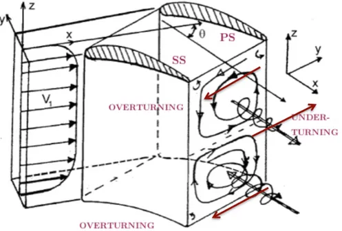
Considering the channel between two adjacent blades of a planar cascade repre-sented in Figure 1.8, it is assumed an orthogonal reference system (x,y,z), where z-axis is parallel to the blade height and x-axis is locally oriented as the meridio-nal velocity of the flow. Furthermore, velocity distribution along z is considered symmetric.

Figure 1.8: Description of a passage vortex given by a non-uniform inlet velocity

profile along the blade height.

The presence of the tip and the hub boundary layers represents the main source of non-uniformity of the flow. More in detail, two counter-rotating vortical structures are generated, mainly the tip passage vortex (TPV) and the hub passage vortex (HPV).

The way in which the passage vortexes are formed is inviscid and their magnitude 8

(23)

1.4 Secondary flows

depends on the non-uniformities of the flow and the inlet flow angle.

When the flow enters into the blade channel, it is subjected to the pressure gradient existing between the pressure side of one blade and the suctions side of the adjacent one. As a consequence, the flow incurs to an increment of the flow deflection both at the hub and tip regions leading to overturning; on the contrary, at the midspan region the passage vortex pushes the flow in the counter-gradient direction, resulting in a reduction of the overall flow deflection, leading in this case to an under-turning. Therefore, the effects of the passage vortexes are mainly a change in the flow direction depending on the radial position and the energy loss as a consequence of the tangential component of the flow velocity transferred to the secondary planes.

Figure 1.9 represents the effect of the interaction between passage vortexes between adjacent blade channel at the cascade outlet.

Figure 1.9: Sheet vortexes at the stage outlet.

The presence of the passage vortexes can increase the losses at the outlet of the blade cascade, where they are in contact with the ones of the adjacent channel; as it is visible from Figure 1.9, these structures are counter-rotating one respect to the other. More in detail, at the contact points, given the viscous nature of these structures, small vorticity cores with a rotation axis parallel to the streamwise direction are generated in order to maintain the continuity. These structures represent the trailing shed vorticity.

Even if passage vortexes are bigger, they dissipated less energy. In fact the dissipa-tion level introduced by a vortex is inversely propordissipa-tional to its size; so the smallest

(24)

Introduction

vortex, the highest viscous stresses since they are characterized by higher angular speed. The largest vortical structures start to fragment generating gradually smaller structures until their scale achieves the Kolmogorov length. In this condition, the velocity gradients are high enough to dissipate all the energy through heat and so smaller vortical structures with respect to the Kolmogorov length scale cannot exist.

1.4.2 Horse-shoe vortexes

When the flow in a turbomachine meets an obstacle in its path, such as the stator and rotor blades, it stops at the leading edge region and deflect in two opposite directions: a branch on the pressure side and another one on the suction side. This process leads to the generation of two counter-rotating vortexes called horse-shoe vortex.

Close to the hub and tip endwalls, in the boundary layers the velocity gradient is normal to the walls, whereas the pressure gradient is null.

Immediately out of the boundary layer, the flow stopped at the leading edge of the blade, is able to recover almost the whole kinetic energy of the undisturbed flow, whereas the recovery close to wall is practically negligible. This process leads to the generation of a pressure gradient and, consequently, a motion of the flow toward the endwalls is initiated.

Figure 1.10: Interaction between horse-shoe and passage vortexes.

As shown in Figure 1.10, the horse-shoe vortex generated on the pressure side of the blade has the same direction of rotation of the passage vortex, so the latter is reinforced and together migrate toward the suction side of the adjacent blade, pushing the horse-shoe vortex initiated on the suction side, that is counter-rotating with respect to the passage vortex, against the blade surface.

(25)

1.4 Secondary flows

1.4.3 Leakage and scraping vortexes

When a relative motion between the blade and the endwalls is present, for example at the tip of the rotor in order to guarantee the rotation or at the hub of the stator close to the rotor shaft, some flow rate draws both in the axial and the tangential directions through the clearance.

The first situation proposed in the two example is detrimental since the blade does not exchange work with the flow, whereas the second one generates some vortexes due to the leakage from the pressure side towards the suction side that interact with other secondary flows. In the case under study, since the stator has an outer casing, it does not show this type of behaviour, even if actually these types of structures are always present due to a minimum clearance but with a negligible contribution in magnitude.

Because of the pressure gradient across each single blade, the tip leakage vortexes always point from the PS towards the SS, both in turbines and compressors independently from direction of rotation of the machine, as observed in Figure 1.11.

Figure 1.11: Interaction between passage, leakage and scraping vortexes for

compressor and turbine blades.

In addition tip leakage vortexes (TLV) are always on the suction side of the blade where they get in touch with both the tip passage vortex (TPV) and the scraping vortex (SV). The latter vorticity structure is linked to the drawing of low energy fluid next to the walls; the mechanism generates a secondary vortex called scraping vortex, which is on the suction side of the blades for turbines.

What is more, the presence of a SV in turbines blade has beneficial effects for the efficiency of overall the stage because it tends to dump the TLV; conversely for compressors, these two vortical structures are on opposite sides of the blade and so they do not interact.

(26)

Introduction

1.4.4 Computational vorticity evaluation

In this section, it is shown how the vorticity is taken into account from the computational point of view.

The vorticity is a vector ω, defined as the curl of the flow velocity v vector. The definition can be expressed by the vector analysis Equation 1.1.

ω= ∇ × v = det    i j k ∂ ∂x ∂ ∂y ∂ ∂z vx vy vz    (1.1)

More in detail, in the present case study the streamwise vorticity is used to isolate secondary vortices. The streamwise component of the voricity could be found by simply scalarly multiplying the vorticity ω with the velocity v and normalizing with respect to v, as shown in Equation 1.2.

Ωs= − 0.0306[m] 4π · 44[m/s] 1 ||v||     ∂vz ∂y − ∂vy ∂z ∂vx ∂z − ∂vz ∂x ∂vy ∂x − ∂vx ∂y     ·    vx vy vz    = = −_{4π · 44[m/s]}0.0306[m] _||v||1 (∂vz ∂y − ∂vy ∂z )vx+ ( ∂vx ∂z − ∂vz ∂x)vy+ ( ∂vy ∂x − ∂vx ∂y)vz ! (1.2) The Equation 1.2 is multiplied by 0.0306[m] and divided by 44[m/s] in order to obtain a non-dimensional variable and so to make a proper comparison with experimental results; more in detail, they correspond respectively to the stator axial chord and to the reference meridional velocity. Finally the negative sign is considered to obtain by convention a positive magnitude for clockwise rotating vortices and a negative one for counter-clockwise rotating vortices, coherently with the sign convention used for the experiments.

1.5 Operating conditions

During the experimental campaign four different operative conditions have been tested as shown in Table 1.3.

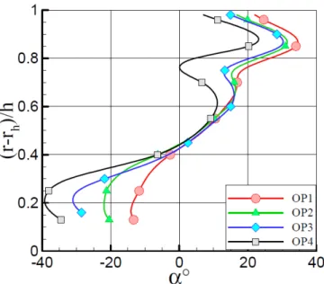
These operative conditions are tested in order to characterize the effect of the expansion ratio, ranging from an almost incompressible (OP4) to a transonic one (OP1) including two intermediates (OP3 and OP2) classified according to the expansion ratio. The coupling between expansion ratio and rotational speed in OP1-4 is chosen in order to have the same absolute flow angle at the stage outlet; since the present turbine has a fully three-dimensional geometry and the secondary flows alter the flow pattern at the endwalls, this constraint is imposed on the midspan region as show in Figure 1.12 [11].

(27)

1.5 Operating conditions

Table 1.3: Operative conditions summary

Figure 1.12: Absolute flow angle downstream of the stage for the different

oper-ating conditions.

OP1 and OP3 are considered the most meaningful operative conditions: as shown in [12], the results for a low speed test in OP4 are much less significant than in OP3 since the analysed quantities are not affected by any significant variation. Furthermore, OP1 is chosen since the test is performed at maximum rotational speed.

In this work, OP1 and OP3 are analysed in reference condition, whereas, when hot streaks injection is considered, only the OP3 is studied since experimental data for OP1 are not available.

(28)

(29)

2. Results of the experimental

cam-paign

2.1 Stator inlet conditions

The stator inlet conditions are measured for all the four injection positions, but the large distance between injectors and the vane ensures to neglect the impact of the stator on the generation of the hot streaks, resulting in identical results for all the cases considered.

Figure 2.1: Temperature ratio between the core of the hot streak and the main

stream (A), and total pressure (B) fields of the hot streak. Pmean is reported as a difference between the local total pressure and the main stream pressure (kinetic head = 1100Pa). (C) RMS of the total pressure.

(30)

Results of the experimental campaign

Figure 2.1 shows the total temperature and total pressure distributions upstream of the stator when the hot streak is injected. Due to the presence of the injector itself, a dynamic pressure perturbation is introduced, producing a non-uniformity in the total pressure field. However this variation results in a negligible variation of the stage pressure ratio.

Figure 2.1A illustrates an almost circular pattern of the hot streak that smooths down radially to the main stream temperature.

Finally in 2.1C, the RMS of the total pressure evidences the turbulent content of the hot streak, given by the interaction of the jet with the surrounding flow and from the injector wake itself. The peak of the RMS is located where the maximum total pressure gradient is depicted, namely where the largest shear layer establishes between the injector wake and the hot streak [6].

2.2 Stator outlet field

In this section, an overview of the thermal fields of all the four cases considered is provided. Generally an important distortion is found caused by the interaction between the hot streak and the stator aerodynamics. The distortion is furthermore followed by a significant reduction of the temperature peak-value (from 1.2 to 1.05 of the main stream total temperature) given by the heat exchange with the surrounding flow and by the diffusion promoted by turbulence and whirling flows inside the blade channel.

Considering now the LE case looking at 2.2A, the hot streak directly impinges on the stator blade leading edge and the blockage represented by the presence of the blade enhances the spread of the temperature all across the span. What is more the temperature profile distribution is stretched on the blade suction side as a consequence of the acceleration and successive deceleration in the blade channel. It has also to be noticed the presence of a region at relatively high temperature on the tip region close to the suction side of the adjacent blade: it is given by the interaction between the hot streak and the cross flow connected to the tip passage vortex, that moves part of the hot streak flow along the casing [6].

Considering now the MP case in Figure 2.2B the hot streak only partially interacts with the wake, but the temperature profile given by the hot streak spreads over a wide portion of the stator channel. Looking at the the tip region close to suction side of the adjacent blade, an interaction with the secondary flow is still visible, even if it is much weaker than in the LE case.

Considering at the end the PS and SS injection cases, it is worth noticing a slightly higher preservation of the hot streak, resulting in a higher temperature peak. It seems also that the wake acts as a boundary for the hot streak diffusion.

Also, for the SS injection case in Figure 2.2C no peak of temperature close to the casing is visible: the interaction with the passage vortex seems to mainly occur

(31)

2.2 Stator outlet field

with the under-turning side of the vortex, which is closer to the midspan. For these reasons, the hot area is stretched toward the pressure side of the adjacent blade.

Finally the hot area in the PS case is pushed toward the hub due to the leaning of the blade, whereas in the SS case it remains close to the tip [6].

Figure 2.2: Total temperature fields downstream of the stator for the four hot

streak positions.

Some considerations should be done about the vorticity fields in different cases. Looking at Figure 2.3A, the hot streaks trigger the onset of two additional vorticity cores in the stator exit flow field at the top and bottom margins of the jets. This is due to the velocity gradients in the shear layer between the hot streak and the main stream. The upper vorticity core enforces both the tip shed vorticity and also the vorticity in the boundary layer; the lower vorticity instead stands isolated. Considering now PS injection, Figure 2.3B, the hot streak induces a positive vorticity area (PV) on the pressure side of the wake. Furthermore, since the hot streak is now closer to the wake with respect to the MP case, a more significant

(32)

Results of the experimental campaign

Figure 2.3: Streamwise vorticity for (A) MP injection, (B) PS injection, (C) SS

injection.

interaction is initiated, enhancing the onset of a local negative vorticity region (NV).

In the case of SS injection, Figure 2.3C, the hot streak affects the flow field in a similar way with respect to PS case: an equivalent amplification of the vorticity magnitude appears on the other side of the wake, in correspondence of the position of the hot streak [6]. The LE injection does not show a specific effect of the hot streak on the stator secondary flow, so it is not reported in Figure 2.3 for sake of simplicity.

(33)

3. Boundary conditions and case

settings

In this chapter boundary conditions and case setups used in all the simulations executed in this work are presented.

Figure 3.1 illustrates the implemented computational domain axially bounded from inlet and outlet planes and tangentially limited from hub and shroud endwalls. The secondary plane on which measurements take place is also reported: it is located at 67.5% of the entire domain along the axial direction.

Finally periodic walls are also considered. Periodic boundary conditions are used when the physical geometry of interest and the expected flow pattern have a periodically repeating nature, as in the case of turbomachines. This means that the flows across two opposite planes in the computational model are identical. A notable reduction of the extension of the model and, consequently, of the computational effort are allowed.

(34)

Boundary conditions and case settings

3.1 OP3 in reference condition

For the reference condition, without hot streaks injection, the measured inlet and outlet quantities are computed through the commercial code ANSYS-CFX. It integrates Reynolds-averaged Navier-Stokes equations with high resolution schemes for convective fluxes under finite-volume, node-centered approach. CFX solver adopts the coupled strategy and algebraic multi-grid method.

The setup for the case prescribes a constant total temperature all over the section at 323K, total pressure distribution (see Figure 3.2A), turbulence intensity equal to 5%, eddy viscosity ratio set at 10 and flow direction normal to the boundary at the inlet; static pressure distribution (see Figure 3.2B) experimentally measured and circumferentially averaged at the outlet; furthermore, no-slip and adiabaticity conditions at walls.

Figure 3.2: Inlet total pressure (A) and outlet static pressure (B) boundary

conditions in OP3.

Regarding the solver, high resolution scheme is selected for the discretization of the term responsible for convective fluxes: ANSYS-CFX schemes are all TVD (total variation diminishing), and specifically high resolution option selftunes the Sweby coefficient for each node individually in order to smooth spurious oscillations that usually affect high accuracy schemes. First order scheme is selected for turbulence.

3.2 OP1 in reference condition

For this operating condition, the setup is almost the same as the previous para-graph: only inlet total pressure and outlet static pressure change. These pressure distributions are visible in Figure 3.3.

(35)

3.3 OP3 with hot streak injection

Figure 3.3: Inlet total pressure (A) and outlet static pressure (B) boundary

conditions in OP1.

3.3 OP3 with hot streak injection

In this section boundary conditions for the hot streak injection case are provided. Total temperature and pressure are derived experimentally as already discussed in Paragraph 2.1 and implemented in CFX. Figure 3.4 illustrates the total temperature and total pressure distributions.

Figure 3.4: Inlet total temperature (A) and total pressure (B) boundary

condi-tions in OP3 with hot streak injection.

More in detail, in Figure 3.4(A), the spot of high temperature generated by the hot streak injection is visible: it shows a peak of temperature equal to 390K at the 70% of the blade height that gradually smears going radially towards the free stream. Figure 3.4(B) instead shows the profile of total pressure that reports the total pressure loss generated by the wake of the injector. The static pressure profile imposed to the outlet is the same represented in Figure 3.2(B). The presence of both total temperature and total pressure variation at the inlet boundary condition induces the formation of a non-uniform distribution of turbulence properties, such

(36)

Boundary conditions and case settings

as turbulence intensity and eddy length scale. Unfortunately measurements for these two parameters are not available and so they are derived analytically. In particular, as already introduced in Paragraph 2.1, measurements about the RMS of the total pressure are available and used in Equation 3.1 that, properly rearranged, allows to obtain an expression for the turbulence intensity. The reader is invited to refer to [13] in order to fully understand the derivation of the Equation 3.1.

P t2

R= 0.49ρ2(1 − 0.175M4)2· u2R

2

+ ρ2_V2_{(1 + 0.5M}2₎2_{· u}2

R (3.1)

where P tR is the RMS of the total pressure, ρ the density, M the Mach number, V

the streamwise velocity and u2

R represents the turbulent kinetic energy.

Once all the quantities are known (P tR from measurements, see Figure 2.1, and all

the other quantities in Equation 3.1 from simulations) it is possible to derive the turbulent kinetic energy by simply solving a second order equation. The turbulence intensity (TI) is derived as follows:

T I =

q

u2

R

V (3.2)

In order to obtain the turbulent intensity distribution to impose at the inlet boundary condition, maximum and minimum values of P tR are used in 3.1 to

calculate u2

Rmax and u2Rmin; at this point T Imax and T Imin are computed through

Equation 3.2 and, finally, all the intermediate values are obtained by linear interpolation following the total temperature distribution since measurements indicate a distribution of total quantities similar to the total temperature one.

Figure 3.5: Inlet turbulence intensity boundary condition in OP3 with hot streak

injection.

(37)

3.3 OP3 with hot streak injection

The results of these calculations are represented in Figure 3.5, where it is possible to observe a maximum value in the core of the hot streak equal to 8% that gradually reduces going out from the zone affected by the injection achieving a minimum value of 2.5%.

Also the eddy length scale has to be imposed at the inlet of the domain. As for the turbulence intensity, it is calculated by linearly interpolating starting from the total temperature. The maximum vortex scale is set to 11mm according to the diameter of the injector; the minimum value, far from the the injector, is set to 0.5mm.

Figure 3.6: Eddy length scale boundary condition in OP3 with hot streak

injec-tion.

Figure 3.6 shows the distribution of the eddies length scale at the inlet of the stator. During simulations, different eddy length scale profiles, based on the total pressure distribution, have been tested leading to no significant variation detected in results.

The reader should be aware that all figures in this paragraph are referred to a mid-pitch injection. In order to obtain the boundary conditions for the other injection positions (leading edge, pressure side and suction side injection) the mesh is relatively rotated with respect to the boundary condition, that instead is kept fixed.

Always no-slip and adiabaticity conditions at walls are imposed. Regarding the solver control, high resolution scheme is selected for both advection scheme and turbulence.

(38)

(39)

4. Stator computational analysis

in reference conditions

In order to create all the meshes in the present work, the commercial software ANSYS-TurboGrid is employed.

All meshes are structured, consisting of hexahedral elements assembled in multi-block architecture. Grids are also consistent with the turbulent model used during calculations: when k-ε turbulent model is applied a value of y+ higher than 30 is

imposed at the walls; instead, when k-ω SST model is used, a unitary value of y+

is imposed at the wall regions.

First calculations regard the stator in reference conditions, without hot streak injection. For these conditions, only k-ω SST turbulent model is used, whereas when hot streaks are considered both models are taken into account.

In order to achieve satisfactory results in reference conditions many meshes are investigated. In the following paragraphs only the most important ones are dis-cussed, explaining how the final mesh is achieved.

4.1 Mesh with no clearance at the hub of the

blade

The starting point is to create a mesh considering a simplified geometry of the stator: the clearance present at the hub trailing edge is removed and no gap is considered with the aim of helping the convergence of the simulation and achieving first results.

Figure 4.1(A) illustrated the inlet view of the blade wall mesh with no gap, whereas Figure 4.1(B) shows a zoom of the hub region. It is possible to denote a refinement of the cells close to hub and shroud regions in order to obtain a unitary value of

y+ in accordance to the turbulence model used, the k-ω SST.

The reader should aware that Figure 4.1 is just a 4-million-mesh sample in order to show the geometry of the blade used during simulations. In fact this mesh is just one out of the four ones used to perform a sensitivity analysis both in OP3 and OP1.

(40)

Stator computational analysis in reference conditions

Figure 4.1: Inlet view of blade wall mesh (A) and zoomed frame of the hub

region (B) with no clearance.

4.1.1 Simulations and sensitivity analysis in OP3

In this paragraph details about the simulations and results in OP3 reference condition are provided.

In order to create the different meshes used for the sensitivity analysis, commercial software ANSYS-TurboGrid is employed to impose the number of cells of the domain. More in particular, it is possible to set both the target of the total number of cells and the number of blade-to-blade planes used to discretize the domain in

(41)

4.1 Mesh with no clearance at the hub of the blade

spanwise direction; as a consequence, fixing the number of blade-to-blade planes, it is possible to control the level of refinement of these planes by varying the total number of cells all over the domain.

Table 4.1 shows the grids used for the present case setting according to the number of cells in blade-to-blade plane (second row), the number of planes used in spanwise direction (third row) and the total number of cells into the domain (fourth row).

Table 4.1: Grids for stator analysis.

All case settings are already analysed in Paragraph 3.1. The following plots represent the behaviour of the circumferential weighted average of parameters of interest: pressure loss coefficient, static pressure, total pressure and Mach number. All these variables are averaged on the mass, except for the static pressure that is averaged on the area.

Figure 4.2: Total pressure loss coefficient circumferential average in spanwise

(42)

Figure 4.3: Mach number circumferential average in spanwise direction in OP3

reference condition for mesh with no clearance.

Figure 4.4: Static pressure circumferential average in spanwise direction in OP3

(43)

Figure 4.5: Total pressure circumferential average in spanwise direction in OP3

As Figure 4.2 and Figure 4.5 show, computational calculations, in agreement with measurements, depict a zone affected by losses at the hub and shroud regions. These losses are the consequences of the presence of secondary flows, given in particular by the tip passage vortex (TPV) and the hub passage vortex (HPV). Focusing on Figures 4.2-4.5 a quite good agreement between simulations and experimental results is achieved specially around the midspan, far from the endwalls. In terms of total pressure, the highest mismatch is present at 86% of the blade height and, in the worst case (defined as the simulation with the highest difference from the experiment profile), is 900Pa.

Considering now the hub region, unfortunately measurements are not available in the zone going from the hub up to the 10% of the span of the blade, but with an imagination effort, it is easy to forecast a total pressure loss (and consequently a total pressure coefficient loss) higher in experiments than in simulations: this is caused by the absence of any clearance that affects instead all the stator blades at the trailing edge. This clearance is responsible for the induction of high level of vorticity in this region and so also for high pressure losses that will affect overall performances of the entire machine.

The trend of the Mach number (see Figure 4.3) is always diminishing as the radius increases in accordance with the radial equilibrium, so as a consequence the static pressure (see Figure 4.4) will be higher as long as the radius is increased.

All meshes illustrated in Table 4.1 are used to achieve the grid independence. In order to accomplish this aim, the 9 million mesh is taken as reference; then the standard deviation between all the other meshes and the reference one is calculated for every parameter considered, as illustrated in Table 4.2.

(44)

Table 4.2: Standard deviation according to different parameters and meshes.

deviation is obtained with the 4 million mesh and so the grid independence can be considered achieved. Despite this consideration the mesh selected for the present work is the one composed of 9 million cells since the available computational effort is such to stand with this dimension, and, more important, because the higher level of refinement on the blade-to-blade planes allows to achieve more accurate results, specially for simulations with the hot streaks injection.

Now the most interesting parameters are plotted through the commercial software ANSYS-CFX and progressively compared with the experimental results. These parameters are represented on the measurement plane at the outlet of the stator where, obviously, also measurements themselves take place.

Figure 4.6: Comparison of the total pressure loss coefficient between (A)

experi-ments and (B) computational results on the measurement plane at the exit of the stator in OP3 reference condition for mesh with no clearance.

In Figure 4.6 the comparison of the total pressure loss coefficient is taken into account. A good match is achieved over the entire secondary plane: looking Figure 4.6(B) the wake is clearly visible at approximately half of the pitch of the cascade and the detected value is about 18%. High pressure losses are also observed at both the endwalls; these zones are not represented in Figure 4.6(A) due to the limits during measurements. Simulations show high losses at the boundary layers

(45)

due to the presence of shear stresses caused by the velocity gradient. More in detail, it is evident the higher thickening of the shroud boundary layer with respect to the one of the hub generated by the higher loading of the tip as a consequence of the leaning effect of the blade.

At the end other regions of losses are represented following the wake toward the tip and the hub; these losses are associated to swirling structures that will be more precisely described in Figure 4.9. Finally a wide region of almost isentropic flow is clearly visible (where the total pressure loss coefficient is zero), that can be acknowledged as the free-stream.

Figure 4.7: Comparison of the static pressure loss coefficient between (A)

exper-iments and (B) computational results on the measurement plane at the exit of the stator in OP3 reference condition for mesh with no clearance.

Figure 4.8: Comparison of the Mach number between (A) experiments and (B)

computational results on the measurement plane at the exit of the stator in OP3 reference condition for mesh with no clearance. Good accordance is also achieved with the static pressure trend normalized with respect to the reference total pressure (equal to 139000Pa) represented in Figure

(46)

4.7. The evolution of the flow field is in accordance with the radial equilibrium and the pressurized regions, almost aligned to the trailing edge of the stator, are the result of the interaction between the PS and SS of the blade.

Figure 4.8 shows the comparison between measured and simulated values of the Mach number. Also in this case a remarkable accordance is obtained. In agreement with the static pressure field, the Mach number increases moving in spanwise direction towards the hub. Three regions of velocity local deficit are depicted respectively in correspondence of the TPV, HPV and the wake. Finally low velocity is obviously observed to both the boundary layers.

Figure 4.9: Comparison of the streamwise vorticity between (A) experiments

and (B) computational results on the measurement plane at the exit of the stator in OP3 reference condition for mesh with no clearance. Now the streamwise vorticity is analysed. This quantity is assumed to be repre-sentative of the secondary vorticity and so the different swirling structures present in the fluid domain can be highlighted.

Observing the comparison between experimental and computational results in Figure 4.9, given the measurement tool limitations, experimental data from the hub up to the 10% of the blade height are not available. In this region weak vortices are found during calculations: the low intensity of the these structures (see Figure 4.9(B)) has to be connected to the absence of the hub clearance in the computational domain. A more precise description of the vorticity field at the hub will be provided in the following paragraphs when, alternately, clearance and gap will be considered. Furthermore, since the blades have a three-dimensional development of lean type, the pressure field is such to push the secondary flows towards the hub region of the channel. This effect is visible both for the wake and swirling structures to close to the hub. Then, two vortices can be identified at the tip region, namely the passage vortex (the one with positive vorticity) and the associated trailing edge shed vortex (the one with negative vorticity).

(47)

4.1.2 Simulations and sensitivity analysis in OP1

With regard to the OP1 conditions, the mesh initially used is the same applied during OP3 calculations. Unfortunately first results provide a value of y+ _slightly

greater than 1 at the walls. In order to solve this drawback, the set value of y+

is decreased achieving a higher level of refinement close to the walls. So globally the architecture of the whole mesh is unchanged with respect to the one shown in Figure 4.1. Consequently the sensitivity analysis is considered equivalent to the one performed in OP3 conditions.

In this case, a focus on the 9M and 9Mbis meshes (see Table 4.1) is considered in order to evaluate the effect of an higher refinement on the spanwise direction with respect to the one on the blade-to-blade planes. The 9Mbis mesh is created by keeping the same number of cells on the blade-to-blade planes of the 4M mesh and doubling the number of these planes along the spanwise direction. The 9M mesh instead is created starting again from the 4M one, but in this case the number of cells on the blade-to-blade planes is doubled and the number of the planes in spanwise direction is kept constant.

The comparison of the results between 9M and 9Mbis mesh is represented in Figures 4.10-4.13. Ignoring for a while the comparison between the experimental results and considering just the two meshes, the integral difference between the two curves of all the parameters in taken into account and this quantity results to be approximately zero. As a conclusion, it is meaningless to operate a refinement in spanwise direction to the detriment of the one on blade-to-blade planes. Furthermore, a too low level of refinement on the blade-to-blade plane is not able to well represent the evolution of the flow field when hot streaks are considered.

(48)

Figure 4.12: Static pressure circumferential average in spanwise direction in OP1

(49)

Considering now the experimental results, the main conclusions already done for the OP3 conditions are valid also for OP1. Total pressure loss coefficient (Figure 4.10), or equivalently total pressure (Figure 4.13), show two main regions of losses at both the endwalls: at the shroud, because of the presence of the TPV and, at the hub, because of the HPV; what is more, also in this case, at the hub higher losses are registered in experiments due to the presence of the clearance at the stator trailing edge of the real machine. Same considerations with respect to the OP3 condition can be done for the Mach number (Figure 4.11) and for the static pressure (4.12), that, in this case, it is normalized with a reference total pressure equal to 192500Pa.

A more detailed distribution of the main parameters is provided on the measurement plane through the software ANSYS-CFX in Figures 4.14-4.17 leading generally to the same conclusions already discussed.

(50)

Figure 4.14: Comparison of the total pressure loss coefficient between (A)

exper-iments and (B) computational results on the measurement plane at the exit of the stator in OP1 reference condition for mesh with no clearance.

Figure 4.15: Comparison of the static pressure between (A) experiments and (B)

computational results on the measurement plane at the exit of the stator in OP1 reference condition for mesh with no clearance.

(51)

Figure 4.16: Comparison of the Mach number between (A) experiments and (B)

computational results on the measurement plane at the exit of the stator in OP1 reference condition for mesh with no clearance.

Figure 4.17: Comparison of the streamwise vorticity between (A) experiments

and (B) computational results on the measurement plane at the exit of the stator in OP1 reference condition for mesh with no clearance.

(52)

4.2 Mesh with clearance at the hub of the blade

Once first results are achieved through the mesh with any kind of gap, the clearance present in real stator blade at the hub trailing edge is now considered in order to get closer to the experimental measurements, especially at the hub region. This mesh is taken and slightly improved from previous studies (graduation thesis by Giada Migliari, Politecnico di Milano, 2015-2016). Improvements regard the correct positioning of the points that define both the leading and trailing edges and a more appropriate refinement of the mesh among the domain. Figure 4.18 shows the mesh used in the present paragraph.

Figure 4.18: Inlet view of blade wall mesh (A) and zoomed frame of the hub

region (B) with the clearance at the hub trailing edge. 38

(53)

4.2 Mesh with clearance at the hub of the blade

The architecture of the mesh with the clearance is generally the same as the one used in the previous paragraphs; with the aim of creating the mesh in the clearance region, a set of layers is clustered in this region and in order to allow this operation, a really small gap all along the hub of the blade is imposed.

As previously specified, the value of y+ _{is limited to a maximum value of 1 close}

to the walls in order to properly use the k-ω SST turbulence model.

4.2.1 Simulations in OP3

In this section the main parameters are provided through their circumferential average distribution in the spanwise direction of the blade and through plots derived from the commercial software ANSYS-CFX as already done for simulations without no gap or clearance at the hub of the stator blade.

In Figures 4.19-4.20 the distribution of the circumferential weighted average of the main parameters is represented: the solid line shows the evolution of the parameters for the mesh with the clearance; the dashed one, instead, refers to the mesh with no gap or clearance.

Obviously the only difference is depicted at the hub region since the two meshes are identical in all the other areas. So all the considerations already done for the mesh with no clearance at both midspan and tip regions are still valid for the present case.

direction in OP3 reference condition for mesh with clearance at the hub of the blade.

(54)

reference condition for mesh with clearance at the hub of the blade.

A computational fluid-dynamic study of the three-dimensional flow in the stator of a gas turbine stage with hot streak injection

Politecnico di Milano

School of Industrial and Information Engineering

Master of Science in Mechanical Engineering

A computational fluid-dynamic study of the

three-dimensional flow in the stator of a gas

turbine stage with hot streak injection

Abstract

Contents

List of Figures

List of Tables

1. Introduction

1.1

Motivations

1.2

Test rig and instrumentation

1.3

3D blade geometry

1.4

Secondary flows

1.4.1

Passage vortexes

1.4.2

Horse-shoe vortexes

1.4.3

Leakage and scraping vortexes

1.4.4

Computational vorticity evaluation

1.5

Operating conditions

2. Results of the experimental

cam-paign

2.1

Stator inlet conditions

2.2

Stator outlet field

3. Boundary conditions and case

settings

3.1

OP3 in reference condition

3.2

OP1 in reference condition

3.3

OP3 with hot streak injection

4. Stator computational analysis

in reference conditions

4.1

Mesh with no clearance at the hub of the

blade

4.1.1

Simulations and sensitivity analysis in OP3

4.1.2

Simulations and sensitivity analysis in OP1

4.2

Mesh with clearance at the hub of the blade

4.2.1

Simulations in OP3