School of Civil and Environmental Engineering
Polo Territoriale di Como
Master of Science in
Environmental and Geomatic Engineering
Thesis Topic:
A First Complete Benchmarking of the New Chinese 30 m resolution
Global Land Cover Dataset (GLC30) and Regional Land Coverage
Datasets in Italy
Supervisor:
Prof. Maria Antonia Brovelli
Assistant Supervisors:
Dr. Monia Molinari
Master’s of Science Thesis by: Eman Hussein Mohamed Hussein
Matricola: 798073
Acknowledgement
First of all I would like to express my deepest sense of gratitude to all the ones who let this work to come out. To all my professors during all the lectures period in this master, thank you all. You have helped me a lot to have a new way to understanding Geomatics filled with new and different visions.
Deeply, I'd like to thank Prof. Maria Antonia Brovelli, the one who always support me and accepting me for this thesis. It has been a great impact to my career; given the semester lecturing I had on Geographical Information System which developed my interest in the Geomatics studies.
Special Thanks also goes to the entire staff members of the Environmental group, Polo Territoriale di Como, especially Dr. Monia Molinari who helped me throughout with this thesis and for her support and time. I am very much indebted to her for the success of my thesis work. Lastly, I'd like to thank all my Friends and Classmates (Irfan, Guhan, Naresh, Natalia,
Aleksandra, Walter, Amr, and Omar) for their commitments to our education, to their help
and support. We shared special moments that I will always cherish, keep it on my heart.
Dedicate
I'd like to thank my family who support me all my life. Give to me light steps in all my life. I kindly thank my mom, the one who always support me with her payers, for her teaching me from the first step on my life until now; god bless her to me.
To my dad, who always been there for me, support me in every step I had taken on my life. Says always to me" I trust in you, you can do more", Thank you dad.
To my sisters Heba, Nahla and Hind, my life flowers. Thank you for your entire support and kindness god blesses them all to me.
Abstract
The production of thematic maps using an image classification is one of the most common applications of remote sensing; such as the production of Land Use and Land cover maps which derived from photo-interpretation of satellite images and Aerial photos. Considerable research has been directed at the various components of the mapping process, including the assessment of accuracy, which is the focused subject of the Thesis.
As the result of the “Global Land Cover Mapping at Finer Resolution” project led by National Geomatics Center of China, the first 30-meters resolution Open Global Land Cover Dataset (named GlobeLand30) have been produced for the years 2000 and 2010. This important dataset is free, open and downloaded through Website:
http://www.globallandcover.com:6677/InfoServer/GLC/DownLoad.aspx?No=0.
The objective of the current study is the assessment of the thematic accuracy of these data on the Italian area by means of a benchmarking with the more detailed land cover open datasets available for many Italian regions. These datasets are independent each other and provided with different thematic classification and resolutions.
The accuracy assessment is based on the cell-by-cell comparison between Italian regional maps and the GlobeLand30 in order to obtain the confusion matrix and all its derived agreement statistics (overall accuracy, producer’s and user’s accuracy, allocation and quantity disagreement, etc.), which help to understand the Classification Quality.
The Thesis presents the Methodology and Procedures for assessing open GlobeLand30. The analysis has been performed in 8 regions across Italy by taking advantage of GRASS, an open-source GIS which offers advanced features for geospatial data processing and analysis. The results of the assessment was very good. This has proven that the combination of open data and open source software provides us a new way for spatial analyses and geographical applications. Keywords: Remote sensing; Classification; Benchmarking; Accuracy assessment.
Sommario
La produzione di carte tematiche mediante tecniche di classificazione d’immagine rappresenta una delle applicazioni più comuni del telerilevamento; un tipico esempio in questo senso è la realizzazione di carte di copertura e uso del suolo a partire da fotointerpretazione di immagini satellitari o aeree. Tra i numerosi studi di ricerca condotti in tale ambito notevole importanza riveste la valutazione dell’accuratezza del processo di classificazione, tema sul quale è incentrato il presente lavoro.
Nell’ambito del progetto "Global Land Cover Mapping at Finer Resolution" guidato dal National Geomatics Center of China, è stato prodotto, per gli anni 2000 e 2010, il primo dataset globale di copertura del suolo con risoluzione 30 metri (chiamato GlobeLand30); questo importante dataset è gratuito, aperto e scaricabile tramite il sito web:
http://www.globallandcover.com:6677/InfoServer/GLC/DownLoad.aspx?No=0.
L'obiettivo del presente studio è la valutazione dell’accuratezza tematica dei dati GlobeLand30 sul territorio italiano attraverso un’analisi comparativa con le più dettagliate carte di copertura del suolo rese disponibili come “open data” da varie regioni italiane; tali dataset sono indipendenti tra loro e caratterizzati da classificazione tematica e risoluzioni diverse.
La stima dell’accuratezza è stata condotta tramite una procedura che, attraverso un confronto cella per cella tra le carte regionali e la GlobeLand30, ha permesso di calcolare la matrice di confusione e derivare da essa una serie di statistiche (accuratezza globale, accuratezza del produttore, accuratezza dell’utente, grado di discordanza tematica e spaziale etc.) in grado di descrivere la qualità della classificazione.
La tesi presenta la metodologia e le procedure adottate per la valutazione di GlobeLand30. Le analisi, condotte in 8 regioni italiane con risultati molto soddisfacenti, sono state eseguite mediante GRASS, GIS open-source che offre funzionalità avanzate per l'elaborazione e l’analisi di dati geospaziali. Lo studio dimostra come la combinazione di open data e software open source possa fornire una nuova possibilità nello svolgimento di analisi spaziali e nello sviluppo di applicazioni geografiche.
Parole Chiave: Telerilevamento; Classificazione: Analisi Comparativa; Valutazione dell’accuratezza.
Table of Content
1 Introduction ... 1
1.1 Global Land cover from space ... 2
1.2 Challenges to validation ... 3
1.3 Finer resolution observation and monitoring of Global land cover with 30 m resolution ... 6
1.3.1 Data pre-processing and Image classification procedure ... 6
1.3.2 Classification System Design ... 11
2 Accuracy assessment ... 19
2.1 Introduction ... 19
2.2 Issues and constraints of concern ... 20
2.3 Basic Approach ... 22
2.4 Thematic Accuracy ... 23
2.4.1 Measures of Accuracy ... 23
3 Benchmarking conducted herein between GLC30 and Italian regional land cover dataset27 3.1 Methodology ... 27
3.1.1 Study Area ... 27
3.1.2 Italian Land cover Data Collection ... 29
3.1.3 Data Processing ... 30
3.1.4 Agreement Measures ... 33
3.2 First case study: Lombardy region ... 35
3.2.1 DUSAF Land Cover Database ... 36
3.2.2 Data Processing ... 37 3.2.2.1 GLC2000-DUSAF1.1 ... 38 3.2.2.2 GLC2010-DUSAF4.0 ... 39 3.2.3 Accuracy Assessment ... 40 3.2.3.1 GLC2000- DUSAF1.1 ... 40 3.2.3.2 GLC2010- DUSAF4.0 ... 46
3.2.4 Lombardy Case Study Conclusion ... 52
3.3 Second Case study: Liguria region ... 53
3.3.1 Liguria land cover layer ... 54
3.3.2 Data Processing ... 55
3.3.2.1 GLC2000-Liguria2000 ... 56
3.3.2.2 GLC2012-Liguria2012 ... 57
3.3.3.2 GLC2010-Liguria2012 ... 64
3.3.4 Liguria Case Study Conclusion ... 69
3.4 Third Case Study: Trentino-Alto Adige Region ... 70
3.4.1 Trentino-Alto Adige Land cover data collection ... 70
3.4.1.1 Prov. Autonomous Trento ... 70
3.4.1.2 Prov. Autonomous Bolzano ... 71
3.4.2 Data Processing ... 71
3.4.2.1 Prov. Autonomous Trento ... 71
3.4.2.2 Prov. Autonomous Bolzano ... 73
3.4.3 Accuracy assessment ... 75
3.4.3.1 Prov. Autonomous Trento ... 75
3.4.3.2 Prov. Autonomous Bolzano ... 79
3.4.4 Trentino-Alto Adige Case study Conclusion ... 84
3.5 Fourth Case Study: Friuli–Venezia Giulia ... 85
3.5.1 Friuli–Venezia Giulia Land cover layer ... 86
3.5.2 Data processing ... 86
3.5.3 Accuracy Assessment ... 88
3.5.4 Friuli–Venezia Giulia Case Study Conclusion ... 94
3.6 Fifth Case Study: Veneto Region ... 95
3.6.1 Veneto Land Cover Database ... 96
3.6.2 Data processing ... 96
3.6.3 Accuracy Assessment ... 98
3.6.4 Veneto Case Study Conclusion ... 104
3.7 Sixth Case Study: Emilia Romagna Region ... 105
3.7.1 Emilia Romagna land cover layer ... 106
3.7.2 Data Processing ... 107 3.7.2.1 GLC2000-Emilia Rom.2003 ... 109 3.7.2.2 GLC2010-Emilia Rom.2008 ... 111 3.7.3 Accuracy Assessment ... 112 3.7.3.1 GLC2000-Emilia Rom.2003 ... 112 3.7.3.2 GLC2010-Emilia Rom.2008 ... 118
3.7.4 Emilia Romagna Case Study Conclusion ... 123
3.8 Seventh Case Study: Sardinia region ... 124
3.8.1 Sardinia Land Cover layer ... 125
3.8.2 Data Processing ... 126
3.8.2.1 GLC2000-Sardinia2003 ... 127
3.8.3 Accuracy Assessment ... 131
3.8.3.1 GLC2000-Sardinia 2003 ... 131
3.8.3.2 GLC2010-Sardinia 2008 ... 137
3.8.4 Sardinia Case Study Conclusion ... 143
3.9 Eighth Case Study: Abruzzo region ... 144
3.9.1 Abruzzo land Cover layer ... 145
3.9.2 Data processing ... 145
3.9.3 Accuracy Assessment ... 147
3.9.4 Abruzzo Case Study Conclusion ... 153
4 Summery ... 154
5 Areas of Future work ... 158
List of Figure
Figure 1: The temporal distribution of Landsat scenes used in the study (N=8929) ... 7
Figure 2: Temporal distribution of Landsat scenes used in this study. Annual distributions (a) and seasonal distribution (b) of scenes. ... 7
Figure 3: Processing level distributions. Levels L1T (brown) and L1G (blue). ... 8
Figure 4: Radiometric processing of Landsat TM and ETM+ scenes ... 9
Figure 5: Classification Workflow ... 9
Figure 6: Layout of a typical confusion or error matrix. ... 22
Figure 7: Italy Regions. ... 28
Figure 8: Italian Land cover Data Collection. ... 29
Figure 9: Rasterization with different resolution and different methods. ... 30
Figure 10: Patching different tiles. ... 31
Figure 11: Data Processing work flow. ... 33
Figure 12: Lombardy Region. ... 35
Figure 13: Overall Workflow of Lombardy region. ... 35
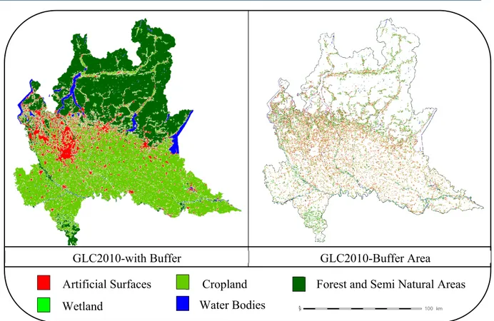
Figure 14: Visual Overview of Both Reclassified DUSAF1.1 and GLC2000 (1st Classification). ... 38
Figure 15: Visual Overview of Both Reclassified DUSAF1.1 and GLC2000 (2nd Classification). ... 39
Figure 16: Visual Overview of Both Reclassified DUSAF4.0 and GLC2010 (1st Classification). ... 39
Figure 17: Visual Overview of Both Reclassified DUSAF4.0 and GLC2010 (2nd Classification). ... 40
Figure 18: First Reclassification Method: Buffer of 70 m eliminated around GLC2000 polygons border (Lombardy2000 Case). ... 44
Figure 19: Second Reclassification Method: Buffer of 70 m eliminated around GLC2000 polygons border (Lombardy2000 Case). ... 45
Figure 20: First Reclassification Method: Buffer of 70 m eliminated around GLC2010 polygons border (Lombardy2012 Case). ... 50
Figure 21: Second Reclassification Method: Buffer of 70 m eliminated around GLC2010 polygons border (Lombardy2012 Case). ... 51
Figure 22: Liguria Region. ... 53
Figure 24: Visual Overview of Both Reclassified Liguria 2000 and GLC2000 (1st
Classification). ... 56 Figure 25: Visual Overview of Both Reclassified Liguria 2000 and GLC2000 (2nd
Classification). ... 57 Figure 26: Visual Overview of Both Reclassified Liguria 2012 and GLC2010 (1st
Classification). ... 57 Figure 27: Visual Overview of Both Reclassified Liguria 2012 and GLC2010 (2nd
Classification). ... 58 Figure 28: First Reclassification Method: Buffer of 70 m eliminated around GLC2000
polygons border (Liguria2000 Case). ... 62 Figure 29: Second Reclassification Method: Buffer of 70 m eliminated around GLC2000 polygons border (Liguria2000 Case). ... 63 Figure 30: First Reclassification Method: Buffer of 70 m eliminated around GLC2010
polygons border (Liguria2012 Case). ... 67 Figure 31: Second Reclassification Method: Buffer of 70 m eliminated around GLC2010 polygons border (Liguria2012 Case). ... 68 Figure 32: Trentino-Alto Adige Region. ... 70 Figure 33: Overall Workflow for Trento Province. ... 71 Figure 34: Visual Overview of Both Reclassified Trento2000 and GLC2000 (1st Classification).
... 72 Figure 35: Visual Overview of Both Reclassified Trento2000 and GLC2000 (2nd Classification).
... 72 Figure 36: Overall Workflow of Bolzano Province. ... 73 Figure 37: Visual Overview of Both Reclassified Bolzano1999 and GLC2000 (1st Classification).
... 74 Figure 38: Visual Overview of Both Reclassified Bolzano1999 and GLC2000 (2nd
Classification). ... 74 Figure 39: First Reclassification Method: Buffer of 70 m eliminated around GLC2000
polygons border (Trento Case). ... 78 Figure 40: Second Reclassification Method: Buffer of 70 m eliminated around GLC2000 polygons border (Trento Case). ... 79 Figure 41: First Reclassification Method: Buffer of 70 m eliminated around GLC2000
Figure 42: Second Reclassification Method: Buffer of 70 m eliminated around GLC2000 polygons border (Bolzano Case). ... 83 Figure 43: Friuli-Venezia-Giulia Region. ... 85 Figure 44: Overall workflow of Friuli-Venezia-Giulia region. ... 86 Figure 45: Visual Overview of Both Reclassified Friuli 2000 and GLC2000 (1st Classification)
... 87 Figure 46: Visual Overview of Both Reclassified Friuli 2000 and GLC2000 (2nd Classification).
... 88 Figure 47: First Reclassification Method: Buffer of 70 m eliminated around GLC2000
polygons border (Friuli2000 Case). ... 92 Figure 48: Second Reclassification Method: Buffer of 70 m eliminated around GLC2000 polygons border (Friuli2000 Case). ... 93 Figure 49: Veneto Region. ... 95 Figure 50: Overall Workflow of Veneto Region ... 95 Figure 51: Visual Overview of Both Reclassified Veneto2009 and GLC2000 (1st
Classification). ... 97 Figure 52: Visual Overview of Both Reclassified Veneto2009 and GLC2000 (2nd
Classification). ... 98 Figure 53: First Reclassification Method: Buffer of 70 m eliminated around GLC2010
polygons border (Veneto Case.) ... 102 Figure 54: Second Reclassification Method: Buffer of 70 m eliminated around GLC2010 polygons border (Veneto2009 case). ... 103 Figure 55: Emilia Romagna Region. ... 105 Figure 56: Overall workflow of Emilia Romagna Region. ... 106 Figure 57: Visual Overview of Both Reclassified Emilia Rom. 2003 and GLC2000 (1st
Classification) ... 109 Figure 58: Visual Overview of Both Reclassified Emilia Rom. 2003 and GLC2000 (2nd
Classification) ... 110 Figure 59: Visual Overview of Both Reclassified Emilia Rom. 2008 and GLC2010 (1st
Classification) ... 111 Figure 60: Visual Overview of Both Reclassified Emilia Rom. 2003 and GLC2010 (2nd
Classification) ... 112 Figure 61: First Reclassification Method: Buffer of 70 m eliminated around GLC2000
Figure 62: Second Reclassification Method: Buffer of 70 m eliminated around GLC2000 polygons border (Emilia Rom. 2003 Case). ... 117 Figure 63: First Reclassification Method: Buffer of 70 m eliminated around GLC2010
polygons border (Emilia Rom. 2008 Case). ... 121 Figure 64: Second Reclassification Method: Buffer of 70 m eliminated around GLC2010 polygons border (Emilia Rom. 2008 Case). ... 122 Figure 65: Sardinia Region. ... 124 Figure 66: Overall Workflow of Sardinia region. ... 125 Figure 67: Visual Overview of Both Reclassified Sardinia 2003 and GLC2000 (1st
Classification). ... 127 Figure 68: Visual Overview of Both Reclassified Sardinia 2003 and GLC2000 (2nd
Classification). ... 128 Figure 69: Visual Overview of Both Reclassified Sardinia 2008 and GLC2010 (1st
Classification). ... 129 Figure 70: Visual Overview of Both Reclassified Sardinia 2008 and GLC2010 (2nd
Classification). ... 130 Figure 71: First Reclassification Method: Buffer of 70 m eliminated around GLC2000
polygons border (Sardinia 2003 Case). ... 135 Figure 72: Second Reclassification Method: Buffer of 70 m eliminated around GLC2000 polygons border (Sardinia 2003 Case). ... 136 Figure 73: First Reclassification Method: Buffer of 70 m eliminated around GLC2010
polygons border (Sardinia 2008 Case). ... 141 Figure 74: Second Reclassification Method: Buffer of 70 m eliminated around GLC2010 polygons border (Sardinia 2008 Case). ... 142 Figure 75: Abruzzo Region ... 144 Figure 76: overall workflow for Abruzzo Region. ... 144 Figure 77: Visual Overview of Both Reclassified Abruzzo2000 and GLC2000 (1st
Classification). ... 146 Figure 78: Visual Overview of Both Reclassified Abruzzo2000 and GLC2000 (2nd
Classification). ... 147 Figure 79: First Reclassification Method: Buffer of 70 m eliminated around GLC2000
polygons border (Abruzzo Case). ... 151 Figure 80: Second Reclassification Method: Buffer of 70 m eliminated around GLC2000
Figure 81: First Reclassification Method, The different Italian Regions classified according to the percentage of Overall accuracy. ... 156 Figure 82: Second Reclassification Method, The different Italian Regions classified according to the percentage of Overall accuracy. ... 157
List of Table
Table 1: Land Cover Classification Classes ... 17
Table 2: Italy Regions. ... 28
Table 3: CORINE land Cover Legend ... 31
Table 4: GLC Legend. ... 32
Table 5: GLC Legend Corresponding to CORINE Legend. ... 32
Table 6: DUSAF Database ... 37
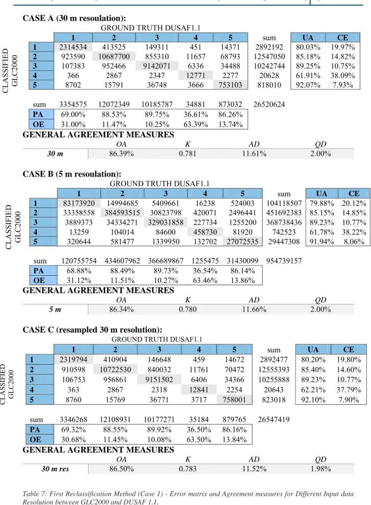
Table 7: First Reclassification Method (Case 1) - Error matrix and Agreement measures for Different Input data Resolution between GLC2000 and DUSAF 1.1. ... 41
Table 8: Second Classification Method (Case2); Agreement measures with 30 m input data resolution Between Reclassified Maps GLC2000 and DUSAF1.1. ... 43
Table 9: General Agreement measures after eliminating the Buffer between reclassified GLC2000 and DUSAF1.1. ... 44
Table 10: GLC2000-DUSAF1.1, Commission and Omission disagreement by pixel (%). ... 45
Table 11: Second Classification Method (Case2); Agreement measures with 30 m input data resolution after eliminating the buffer between reclassified GLC2000 and DUSAF1.1. ... 46
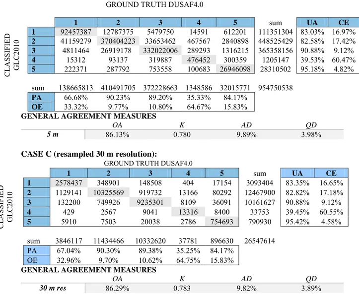
Table 12: First Reclassification Method (Case 1) - Error matrix and Agreement measures for Different Input data Resolution between GLC2010 and DUSAF 4.0. ... 47
Table 13: Second Classification Method (Case2); Agreement measures with 30 m input data resolution between reclassified Maps GLC2010 and DUSAF4.0. ... 49
Table 14: General Agreement measures after eliminating the buffer between reclassified maps GLC2010 and DUSAF4.0. ... 50
Table 15: GLC2000-DUSAF4.0, Commission and Omission disagreement by pixel (%) ... 51
Table 16: Second Classification Method (Case2); Agreement measures with 30 m input data resolution after eliminating the buffer. ... 52
Table 17: Liguria Land cover layers. ... 54
Table 18: First Reclassification Method (Case 1) - Error matrices and Agreement measures for Different Input data Resolution between GLC2000 and Liguria2000. ... 59
Table 19: Second Classification Method (Case2); Agreement measures between compared maps GLC2000 and Liguria 2000 with 30 m input data resolution. ... 61
Table 20: General Agreement Measures between Reclassified GLC2000 and Liguria2000 after the Elimination of a Buffer. ... 62
Table 22: Second Classification Method (Case2); Agreement measures with 30 m input data resolution after eliminating the buffer between reclassified GLC2000 and Liguria2000. ... 63 Table 23: First Reclassification Method (Case 1) - Error matrices and Agreement measures for Different Input data Resolution between GLC2010 and Liguria2012. ... 65 Table 24: Second Classification Method (Case2); Agreement measures between reclassified maps GLC2010 and Liguria 2012 with 30 m input data resolution. ... 66 Table 25: General Agreement Measures between Reclassified GLC2010 and Liguria2012 after the Elimination of a Buffer. ... 67 Table 26: GLC2000-Liguria2000, Commotion and Omission Disagreement by pixel%. ... 67 Table 27: Second Classification Method (Case2); Agreement measures with 30 m input data resolution after eliminating the buffer between reclassified maps GLC2010 and Liguria2012. 68 Table 28: First Reclassification Method (Case 1) - Error matrices and Agreement measures for Different Input data Resolution between GLC2000 and Trento2000. ... 75 Table 29: Second Classification Method (Case2); Agreement measures with 30 m input data resolution between GLC2000 and Trento2000. ... 77 Table 30: General Agreement Measures after Eliminating the Buffer (Trento Case). ... 78 Table 31: GLC2000-Trento2000, Commission and Omission disagreement by pixel %. ... 78 Table 32: Second Classification Method (Case2); Agreement measures with 30 m input data resolution after eliminating the buffer (Trento Case). ... 79 Table 33: First Reclassification Method (Case 1) – Error matrices and Agreement measures for Different Input data Resolution between GLC2000 and Bolzano1999. ... 80 Table 34: Second Classification Method (Case2); Agreement measures with 30 m input data resolution between GLC2000 and Bolzano1999. ... 82 Table 35: General Agreement Measures after Eliminating the Buffer (Bolzano Case). ... 83 Table 36: GLC2000-Bolzano1999, Commission and Omission disagreement by pixel %. ... 83 Table 37: Second Classification Method (Case2); Agreement measures with 30 m input data resolution after eliminating the buffer (Bolzano Case). ... 84 Table 38: Friuli land cover layer ... 86 Table 39: First Reclassification Method (Case 1) - Error matrices and Agreement measures for Different Input data Resolution between GLC2000 and Friuli 2000. ... 89 Table 40: Second Classification Method (Case2); Agreement measures between reclassified GLC2000 and Friuli2000 with 30 m input data resolution. ... 91 Table 41: General Agreement measures after elimination of Buffer between Reclassified GLC2000 and Friuli2000. ... 92
Table 42: Friuli2000, Commission and Omission disagreement by pixel%. ... 92 Table 43: Second Classification Method (Case2); Agreement measures with 30 m input data resolution after eliminating the buffer (Friuli2000 Case). ... 93 Table 44: Veneto Land Cover Layer. ... 96 Table 45: First Reclassification Method (Case 1) - Error matrices and Agreement measures for Different Input data Resolution between GLC2010 and Veneto2009. ... 99 Table 46: Second Classification Method (Case2); Agreement measures between compared maps GLC2010 and Veneto2009 with 30 m input data resolution. ... 101 Table 47: General Agreement Measures between GLC2010 and Veneto2009 after the
Elimination of a Buffer. ... 102 Table 48: GLC2010-Veneto2009, Commotion and Omission Disagreement by pixel%. ... 102 Table 49: Second Classification Method (Case2); Agreement measures with 30 m input data resolution after eliminating the buffer (Veneto2009 Case). ... 104 Table 50: Emilia Romagna Land cover Database. ... 106 Table 51: First Reclassification Method (Case 1) - Error matrices and Agreement measures for Different Input data Resolution between GLC2000 and Emilia Rom. 2003 ... 113 Table 52: Second Classification Method (Case2); Agreement measures between compared maps GLC2000 and Emilia Rom. 2003 with 30 m input data resolution. ... 115 Table 53: General Agreement Measures between GLC2000 and Emilia Rom. 2003 after the Elimination of a Buffer. ... 116 Table 54: GLC2000-Emilia Rom. 2003, Commotion and Omission Disagreement by pixel%. ... 116 Table 55: Second Classification Method (Case2); Agreement measures with 30 m input data resolution after eliminating the buffer between reclassified maps GLC2000-Emilia Rom.2003. ... 117 Table 56: First Reclassification Method (Case 1) - Error matrices and Agreement measures for Different Input data Resolution between GLC2010 and Emilia Rom. 2008. ... 118 Table 57: Second Classification Method (Case2); Agreement measures between compared maps GLC2010 and Emilia Rom. 2008 with 30 m input data resolution. ... 120 Table 58: General Agreement Measures between GLC2010 and Emilia Rom. 2008 after the Elimination of a Buffer. ... 121 Table 59: GLC2000-Emilia Rom. 2003, Commotion and Omission Disagreement by pixel%. ... 122
Table 60: Second Classification Method (Case2); Agreement measures with 30 m input data resolution after eliminating the buffer between reclassified maps GLC2010-Emilia Rom.2008. ... 123 Table 61: Land Cover layer of Sardinia region. ... 125 Table 62: First Reclassification Method (Case 1) - Error matrices and Agreement measures for Different Input data Resolution between GLC2000 and Sardinia2003. ... 131 Table 63: Second Classification Method (Case2); Agreement measures between compared maps GLC2000 and Sardinia 2003 with 30 m input data resolution. ... 134 Table 64: General Agreement Measures between GLC2000 and Sardinia 2003 after the
Elimination of a Buffer. ... 135 Table 65: GLC2000-Sardinia 2003, Commotion and Omission Disagreement by pixel%. .... 136 Table 66: Second Classification Method (Case2); Agreement measures with 30 m input data resolution after eliminating the buffer between reclassified maps GLC2000-Sardinia.2003. . 137 Table 67: First Reclassification Method (Case 1) - Error matrices and Agreement measures for Different Input data Resolution between GLC2010 and Sardinia2008. ... 138 Table 68: Second Classification Method (Case2); Agreement measures between compared maps GLC2010 and Sardinia 2008 with 30 m input data resolution. ... 140 Table 69: General Agreement Measures between GLC2010 and Sardinia 2008 after the
Elimination of a Buffer. ... 141 Table 70: GLC2000-Sardinia 2003, Commotion and Omission Disagreement by pixel%. .... 142 Table 71: Second Classification Method (Case2); Agreement measures with 30 m input data resolution after eliminating the buffer between reclassified maps GLC2010-Sardinia.2008. . 143 Table 72: Abruzzo land cover layer. ... 145 Table 73: First Reclassification Method (Case 1) - Error matrices and Agreement measures for Different Input data Resolution between GLC2000 and Abruzzo2000. ... 148 Table 74: Second Classification Method (Case2); Agreement measures between compared maps GLC2000 and Abruzoo2000 with 30 m input data resolution. ... 150 Table 75: General Agreement Measures between GLC2000 and Abruzzo2000 after the
Elimination of a Buffer. ... 151 Table 76: GLC2000-Abruzzo2000, Commotion and Omission Disagreement by pixel%. ... 151 Table 77: Second Classification Method (Case2); Agreement measures with 30 m input data resolution after eliminating the buffer (Abruzzo Case). ... 152
List of Equation
Equation 1: Overall Accuracy. ... 23
Equation 2: User Accuracy. ... 24
Equation 3: Commission Error. ... 24
Equation 4: Producer Accuracy. ... 24
Equation 5: Omission Error. ... 24
Equation 6: Kappa Standard. ... 25
Equation 7: Allocation Disagreement. ... 25
1
INTRODUCTION
.
Land cover, and human and natural alteration of land cover, play a major role in global-scale patterns of the climate and biogeochemistry of the earth system. Terrestrial ecosystems exert considerable control on the planet’s biogeochemical cycles, which in turn significantly influence the climate system through the radiative properties of greenhouse gases and reactive species. Further, variations in topography, albedo, and vegetation cover, and other physical characteristics of the land surface influence surface-atmosphere fluxes of sensible heat, latent heat, and momentum, which in turn influence weather and climate (Sellers et al., 1997)i. Reliable
information on the state of our planet’s land cover is thus needed on a regular basis if we are to understand the balance between global land cover patterns, climate, and changes occurring in either of these. Despite the significance of land cover as an environmental variable, our knowledge of land cover and its dynamics is poor. Understanding the significance of land cover and predicting the effects of land cover change is particularly limited by the paucity of accurate land cover data.
Land-cover data are some of the most important variables in all nine societal benefit areas that the Global Earth Observation System (Herold et al. 2008)ii. Until recently, land-cover data sets
used within models of global climate and biogeochemistry were derived from pre-existing maps and atlases. The most commonly used data sets were compiled by Olson and Watts (1982)iii,
Matthews (1983)iv, and Wilson and Henderson-Sellers (1985)v. While these (and other) data
sources provided the best available source of information regarding the distribution of global land cover at the time, several limitations are inherent in their use. For example, global land cover is intrinsically dynamic.
Therefore, the source data upon which these maps were compiled is now out of date in many areas. Further, each of these data sets utilize different spatial scales and classification schemes, which are generally different from those required by contemporary models. As a result, confusion regarding how the reference class units are translated to the classification system and scale used by a model can lead to errors in the final product. For example, floristic and climatically based classifications, while not inherently compatible, may need to be combined and reclassified to generate physiognomic cover types (Townshend, Justice, Li, Gurney, & MacManus, 1991)vi.
Finally, conventional land cover data sets such as those mentioned above often provide maps of potential vegetation inferred from climatic variables such as temperature and precipitation. In many regions, especially where humans have dramatically modified the landscape, the true vegetation type or land cover can deviate significantly from the potential vegetation.
1.1
G
LOBALL
AND COVER FROM SPACEMore recently, remote sensing has been used as a basis for mapping global land cover, large volumes of high-quality global remotely-sensed data have become available, provided by such orbiting instruments as SPOT-Vegetation (CNES, 2000)vii, MODIS (Justice et al., 1998)viii, and
MERIS (ESA, 2004)ix. These imagers provide near-daily multispectral imaging of the Earth’s
land surface at resolutions ranging from 250 to 1000 m. Their frequent coverage provides a higher probability of observing the surface without interference from clouds, thus allowing the construction of global datasets in which nearly all points on the Earth’s land surface have been imaged on multiple occasions. This, in turn, opens the door for global science data products derived from multispectral and multi-temporal measurements.
Among these science data products is global land cover, typically presented as a digital thematic map in raster format with pixels in the range of 500-1000 m. Thus far, six types of global land-cover maps derived from remotely sensed data are freely available:
1. The 1 km International Geosphere-Biosphere Programme Data and Information System Cover (IGBP-DISCover) map was produced from monthly normalized difference vegetation index (NDVI) composites derived from 1992 to 1993 National Oceanic and Atmospheric Administration (NOAA) Advanced Very High Resolution Radiometer (AVHRR) data (Loveland et al. 2000)x. An unsupervised classification method was used
to produce this map.
2. The 1 km University of Maryland (UMD) land-cover map was produced with the same data set as mentioned above (Hansen et al. 2000)xi. A supervised classification tree
method was used to produce this map.
3. The 1 km Global Land Cover 2000 (GLC2000) map was produced from monthly NDVI data derived from 1999 to 2000 Satellite Pour l’Observation de la Terre (SPOT) vegetation data (Bartholome and Belward 2005)xii. It was produced by people working
separately, in parallel, on 19 different regions of the world using various types of algorithms.
4. 500 m Moderate Resolution Imaging Spectrometer (MODIS) land-cover maps are now being generated annually with MODIS data (Friedl et al. 2002, 2010)xiii. Recently, a
supervised classification tree algorithm has been used to produce these maps.
5. 300 m GlobCover land-cover maps were produced with bimonthly Medium Revolution Imaging Spectrometer (MERIS) data mosaics derived from the Environmental Satellite (ENVISAT) for 2005 and 2009 (Arino et al. 2008; Bontemps et al. 2010)xiv. They were
produced with an automatic multi stage classification procedure using spectral–temporal and phonological information with an unsupervised classification method.
6. The 1 km MODIS land-cover map was derived from the MODIS 1 km monthly product led by Japan through international collaboration (Tateishi et al. 2011)xv. A combination
of supervised classification and single-class extraction algorithms was used to make this map.
The classification schemes used by the three US global land cover products (IGBPDISCover, UMD, MODIS) used the IGBP classification system with 17 categories of cover types, whereas the two European products (GLC2000, GlobCover) used a 22 category classification scheme that was developed for similar purposes by the IGBP system in order to meet global modelling purposes. This has come about through a standard class definition and aggregation system developed by the Food and Agriculture Organization (FAO) (Di Gregorio 2005)xvi.
1.2
C
HALLENGES TO VALIDATION
In many applications, remotely-sensed global land cover maps are simply ingested without concern for their quality or accuracy. The rationale for this action is often that conventional sources of land cover information are so generalized that anything is an improvement. Another factor leading to unquestioned use is that other uncertainties may have a greater effect on the modeled outcome than errors in land cover information. In either case, land cover maps are being used without an appreciation of their inherent uncertainties, which may be large. It is clear that users of land cover information can improve their products and predictions by having some knowledge of the error structure of the land cover data in use. Moreover, global land cover maps differ significantly, depending on the quality of the input data and the classification algorithm used to produce them, as well as the spatial resolution and legend (Townshend, et al., 1991)xvii.
Given this variation, the choice of a particular map may substantially affect user’s outputs. All land-cover products were generated by computer classification algorithms of different types but on a per-pixel basis.
The term validation as a suite of techniques for determining the quality of a particular map. The techniques include assessing the accuracy of a given map based on observations such as overall accuracy, errors of omission and commission by land cover class, errors analyzed by region, and fuzzy accuracy (probability of class membership), all of which may be estimated by statistical sampling. Although the validation techniques we will describe rely heavily on probability sampling designs for collecting validation data, information obtained without a proper statistical sample design will often be useful in understanding the basic error structure of the map. Such information includes spatially-distributed confidence values provided by classification algorithms, as well as systematic qualitative examinations of the map and comparisons (both qualitative and quantitative) with other maps and data sources.
The overall accuracy (OA) of the IGBP DISCover map was 66.9% (Scepan 1999)xviii, and the
GLC2000 map was 68.6% (Mayaux et al. 2006)xix. Cross-validated OA (using training data) for
the MODIS product was 78.3% (Friedl et al. 2002) and 77.9% for GlobCover based on 2186 random samples of homogeneous land covers (Arino et al. 2008). Through international collaboration, Tateishi et al. (2011) made use of reference map data from over 180 countries. They developed their own classification scheme with 20 classes. Using a validation data set of 600 points, they reported an OA of 76.5%.
In spite of these validation assessments, some third-party researchers have found considerably lower accuracies in different parts of the world when verifying the various global land-cover products (Gong 2009a; Fritz, See, and Rembold 2010)xx. Using 400 field survey points to assess
the MODIS land-cover product, Sedano, Gong, and Ferrao (2005)xxi found greater than 50%
error in the Mozambique Miombo ecosystem over an area of approximately 100,000 km2. Using
over 2000 field samples collected in Siberia covering approximately 1 million km2, Frey and
Smith (2007)xxii found that the OAs for the IGBP DisCover and MODIS global land-cover
products were 22% and 11%, respectively. From a global comparison of the IGBP DISCover, UMD, MODIS, and GLC2000 data products, it was found that relatively consistent results can be found only over the snow and ice fields of Greenland, the desert areas in Africa, and the rain-forests of the Amazon Basin, areas occupying 26% of the global land surface (MaCallum et al. 2006)xxiii. From seven selected 500 km × 500 km comparison areas, in Africa, Asia, Australia,
Europe, North America, Russia, and South America, the consistencies among these four global land-cover products for all but South America were below 20%. Using 250 Fluxnet sites, Gong (2009a) found that the OAs of the first three global land-cover maps produced with the IGBP classification system were below 42%. Previous research found that accuracies for different land-cover categories varied greatly, with evergreen broadleaf forest and desert areas best classified, but heterogeneous land-cover areas poorly classified (Jung et al. 2006; Herold et al. 2008)xxiv.
It seems that so far only the evergreen broadleaf and the snow and ice cover classes have been reliably mapped with certainty. Mixed trees, deciduous broadleaf trees, shrub, and herbaceous land covers are the most confused classes (Herold et al. 2008; Sterling and Ducharne 2008)xxv.
A spatial consistency check revealed that tropical forest, barren, and snow and ice cover classes are mapped homogeneously, but many transitional zones have low classification accuracies where finer resolution data are called for (Herold et al. 2008; Tchuente, Roujean, and de Jong 2011)xxvi. It was believed that improving the mapping of heterogeneous landscapes is the most
significant challenge for improving global land cover mapping. Future efforts based on finer resolution data may provide improvements’ (Herold et al. 2008). However, this does not come without significant costs for data, local knowledge, and detailed field data.
Current trends in land-cover classification have shifted from a single general purpose classification to individual class information extraction for human settlements (Imhoff 1997; Lu et al. 2008; Schneider et al. 2010; Wang et al. 2010)xxvii, agricultural lands (Ramankutty and
Foley 1998, 1999; Thenkabail et al. 2009)xxviii, wetlands (Niu et al. 2009; et al. 2010; Gong et
al. 2010), lakes (Sheng, Shah, and Smith 2008)xxix, wild-land fires (Pu et al. 2007; Chuvieco,
Giglio, and Justice 2008)xxx, and quantification of vegetation cover fractions (DeFries,
TownShend, and Hansen 1999; Hansen, DeFries, and Townshend 2002; Clinton et al. 2009)xxxi.
In addition, classification algorithms have increased from simple statistical classifiers like the widely used maximum likelihood classifier (MLC), to classification trees (such as the seminal CART and C4.5) to more computationally demanding machine learning classifiers such as support vector machines (SVM) and ensemble classifiers such as Random Forest (RF), and other bagged or boosted classifiers (Witten and Frank 2005)xxxii.
Due to the improvement of computational efficiency, it is now easier to employ and compare results from a number of different classifiers in a mapping task (e.g. Carreiras, Preira, and Shima bukuro 2006; Clinton et al. 2009)xxxiii. In the meantime, more and more ancillary information and
remotely sensed data from different sources are being used in land-cover classification (e.g. Aksoy et al. 2009)xxxiv. From a global perspective, data provided for browsing purposes in virtual
globes, particularly Google Earth, have proved useful for their geometric precision and large volumes of high spatial resolution data available at better than 1 m level (Yu and Gong 2012)xxxv.
In summary, existing global land-cover maps derived from remote sensing were all based on time series of coarser resolution satellite data. The time series is usually for a specific year. Recent advances in data acquisition, data accessibility, and high-performance computing make it possible to use finer spatial resolution data for global land-cover mapping.
In particular, as more Landsat-level data are made freely accessible, it is natural to consider adopting such medium resolution data for global land-cover mapping purposes. Although it is still hard to collect medium resolution data for the entire globe in a consistent season or a year, it is possible to use such data in multiple years to cover the entire globe. Townshend et al. (2012) reported their efforts in mapping global forest cover and monitoring forest changes using Landsat data. They found that atmospheric interference, terrain effects, selecting data from the appropriate season in a year, and training sample selection are particularly challenging.
Despite these difficulties, globally consistent land-cover data from medium resolution satellite sensors that are an order of magnitude finer than weather satellite sensors have never been produced, but they are badly needed for many reasons. First, land process models at regional and global scales need better surface cover fraction data that coarser resolution data cannot provide. Second, although land-cover data at the medium resolution exist, in many developed countries, their classification schemes vary widely making them hard to crosswalk for cross-regional studies such as water resources management in international river basins, conservation of wildlife and biodiversity, and carbon sequestration planning through afforestation. This requires a global land-cover map with a consistent land-cover classification scheme. Third, many developing countries in Africa and Asia do not have land-cover data at this scale. A global land-cover map can fill this gap.
1.3 F
INER RESOLUTION OBSERVATION AND MONITORING OFG
LOBAL LANDCOVER WITH
30
M RESOLUTION1The first efforts in mapping global land cover with 30 m resolution Landsat Thematic Mapper (TM) and Enhanced TM plus (ETM+) data. This was carried out under Finer Resolution Observation and Monitoring of Global Land Cover (FROM-GLC) project. The long-term goal in FROM-GLC is to develop a multiple stage approach to mapping global land cover so that the results can better meet the needs of land process modelling and other application needs mentioned earlier that global Landover maps produced with coarser resolution data failed to meet. The FROM-GLC project should also be easily cross walkable to existing global land-cover classification schemes.
The first step maps broad land-cover categories based on spectral data only. It is meant to serve as a benchmark for future improvements when spatial and temporal and other ancillary features are combined. As Landsat-like data are being made more frequently available, optimal dates for data selection and multi-seasonal data in the same year cannot be used in the future.
1.3.1 Data pre-processing and Image classification procedure
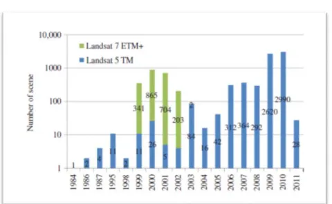
A total of 8929 Landsat TM/ETM+ scenes were collected from various sources (Figures 1 and 2). A total of 2181 scenes were collected from the Global Land Cover Facility (GLCF) at the UMD, 6229 scenes were collected from United States Geological Survey (USGS) Earth Resources Observation and Science (EROS) data center, and an additional 519 scenes were collected from the Satellite Ground Station of China. About 74% of the imagery was acquired after 2006, while images available before 2006 were used as substitutes for places where no suitable imagery could be found after 2006 at the time of the project initiation.
Figure 1: The temporal distribution of Landsat scenes used in the study (N=8929)
Figure 2: Temporal distribution of Landsat scenes used in this study. Annual distributions (a) and seasonal distribution (b) of scenes.
Only 18 scenes acquired before 1998 were used. As a result, approximately three quarters of the imagery is circa 2010 and one quarter is circa 2000. Most of the scenes except those covering China were processed to level L1T (orthorectified), while 161 scenes at higher latitudes were processed to level L1G (non-orthorectified, Figure 3). Only geometrical correction was applied to the images covering China. Since the non-orthorectified images were mainly taken over relatively flat areas, terrain effects were considered negligible where orthorectified imagery was unavailable. A total of 40 scenes were randomly selected to evaluate the geometric discrepancy against Google Earth images. In each scene, 10 ground control points were selected from typical locations to calculate a root mean square error (RMSE). Only one scene in Russia near the Arctic had an RMSE of 2.76 pixels. The remaining RMSEs were below 1.43 pixels. On average, the RMSE was 1.01 pixels, indicating an acceptable geometric agreement between the Landsat images and Google Earth images.
Figure 3: Processing level distributions. Levels L1T (brown) and L1G (blue).
Except those images from the GLCF that were already radiometrically corrected to reduce atmospheric and topographic effects, all remaining L1T images from USGS were radiometrically corrected using software (Figure 4).
The overall work flow of the global land-cover classification is shown in Figure 5. It involves data pre-processing, training, and test sample collection, image classification on a scene-by-scene basis using local training samples from spatio-temporal neighborhood scenes, and finally accuracy assessment.
The radiometric processing was done automatically using the Global Mapper (GM) software package developed by chines that enables image processing coupled with Google Earth image display and visualization. This processing includes atmospheric correction and topographic correction. The final product is images of reflectance with the atmospheric and topographic effects substantially reduced. After automatic processing, manual checking was carried out to ensure correction quality. Scenes with a poor quality correction were re-processed with manually selected parameter sets.
Atmospheric correction was done with an enhanced version of the Fast Line-of-Sight Atmospheric Analysis of Spectral Hyper-cubes (FLAASH) algorithm (Alder-Golden et al. 1999)xxxvi implemented in the GM. Parameter setup was automatically generated based on the
acquisition time and location information from the imagery and ancillary data. Data
Collection Data unzip and
check Radiometric calibration TM/ETM+ DATA Metadata Atmospheric correction Atmospheric parameter Topographic correction Processed Data p001r 002_7dt_20000914_Rad_Ref_TRC.img Processing level Naming Conventions Global Global Path/row Sensor type Acquisition date Radiometric Atmospheric Topographic Extension name
Processed Data Training sample Collection Validation sample Collection
Classification Classifiers (MLC, J84,RF,SVM) Spatial Temporal neighborhood sampling Check Check Accuracy Assessment Using self-collected samples
Figure 5: Classification Workflow
For example, the elevation information was obtained from the Geospatial Image Pyramid (GIP) of the global digital elevation model (DEM) data (recognizable by Google Earth and Environment for Visualizing Images (ENVI)). Aerosol data are inferred from the location information of each scene and DEM data. The GM FLAASH module also contains an automatic processing and optimization mechanism. When it detects over-correction of the imagery, indicated by a large quantity of 0 values, it automatically adjusts the water vapour and aerosol parameters, feeding the optimized parameters back into the atmospheric correction. After the atmospheric correction, the optimized parameters are recycled for use by the topographic correction procedure.
The topographic correction is based on the TopoRadCor procedure in GM. TopoRadCor takes the output from the atmospheric correction and uses the 90 m DEM from the GIP as input. The solar incidence angle is computed based on the DEM and the location and local time information for each pixel. The topographic correction can reduce the distortion over higher latitudes and complex terrain. TopoRadCor automatically adjusts to surface cover type, resulting in a well-characterized surface structure that overcomes over-correction effects
Although many processed scenes have been collected, by the time of training and test sample collection, there were still 656,889 km2 of terrestrial land areas (excluding Antarctica and
Greenland) not covered. These areas were mostly distributed within the Arctic region. Canada, the USA, Russia, and Norway (Svalbard) were among the top four countries with the largest un-mapped areas. Among the 8929 scenes used in this project, 192 scenes were sampled twice by different interpreters due to overlap in separate national and continental mapping task assignments. A total of 1007 scenes (including those 192 scenes mentioned above) share the same Path/Row collected at different times. Training samples were collected on all these images resulting in higher sample density over those overlap areas.
Four types of classifiers were experienced: the traditional MLC, a simple J4.8 decision tree classifier (an improved version of C4.5), support vector machine (SVM) classifier, and RF classifier (Bradski 2000; Hall et al. 2009; Chang and Lin 2011)xxxvii. The MLC was used as a
reference for its popularity, computational simplicity, and robustness. Recently, The SVM classifier has been widely reported as an outstanding classifier in remote sensing (Huang, Davis, and Townshend 2002; Liu, Kelly, and Gong 2006)xxxviii. The RF classifier was tested due to its
reported performance in the machine learning community (Bauer and Kohavi 1999; Caruna and Niculescu-Mizil 2006)xxxix.
Representative sample collection is the most time-consuming and labor-intensive process in the global land-cover mapping effort. Limited by human power, we could not collect as many training samples as we would have liked for each class in every scene. We used samples collected in neighboring scenes to augment training samples. Training samples collected from any particular scene were pooled with samples from a certain number of neighboring scenes and were used to train a classifier for that particular scene. This is not usually needed in training sample
The selection rule is set to be 30 neighboring scenes that meet the spatial and temporal criteria. The search for spatial neighbor images is limited within each of the Eco regions as defined by the World Wildlife Fund (Olson et al. 2001)xl. Temporal neighbor images are based on the
acquisition date of images. At first, image acquisition time is ± 30 days from the current image. If 30 neighborhood scenes cannot be found, the time is relaxed to ±60 days. If 30 neighborhood scenes are still not available, the time is further relaxed to ± 90 days. If still 30 neighborhood scenes cannot be found, use what is available. All bands except the thermal band of the TM or ETM+ images were used in the classification.
1.3.2 Classification System Design
Existing global land-cover maps were produced for different purposes from different types of data with different types of algorithms. Some were developed by different groups of creators. Their classification schemes and implementations are also inconsistent. As a result, a thorough comparison of different land-cover maps is challenging if not impossible. Even so, some efforts have been made to crosswalk and compare these results (Herold et al. 2008; Tateishi et al. 2011). Based on the analysis of existing classification systems, we found that there are major limitations to using a composite class type that combines vegetation trait, structure, and life-form information in a fixed manner. Taking the IGBP, GLC2000, and GLOBCover classification systems as examples, although the three systems differ in some details, they have high consistency as well. All vegetation categories contain life form, canopy closure, and height specifications, but different thresholds within a category. The IGBP system specifies that woody vegetation under 2 m height is classified as shrubs whereas the height limit was increased to 3 m in the GLC2000 and 5 m in the GlobCover classification systems.
Similarly, the canopy closure in different vegetation classes varied among the classification systems. Most land-cover classification systems do not include the distinction between C3 and C4 photosynthetic types but they are needed for land surface process models (DeFries et al. 1995; Dai et al. 2003)xli. However, such information is hard to obtain from remotely sensed data.
Additional data sources or bio-geographical modelling results are often considered for obtaining such information (Stirling and Ducharne 2008)xlii.
In GLC design, it was chosen to build a system separating the trait, life form, and structural information into distinct layers, retaining the original quantitative structural information as much as possible. Traits, life form, and structural data were treated as basic building blocks towards the construction of a complete classification system. These building blocks called end-components. There are a total of 10 land-cover types and eight life form or PFT classes. Canopy closure and heights can be preserved in unclassified form in their original quantities. As the nominal cover-type end-component from canopy closure and height end-components that can be quantitatively characterized were de-coupled.
Any land-cover class can resolve in a new classification system that contains those quantitative end-components. In fact, different types of end-components should be derived from different sources of data or by different types of algorithms. For example, the canopy closure can be derived by applying linear unmixing or regression techniques (Gong, Miller, and Spanner 1994; Roberts et al. 1998; Hansen, DeFries, and Townshend 2002)xliii to the spectral data, whereas
vegetation height information can be obtained from other sources of data such as stereo pairs of images (Gong 2002)xliv, interferometry of synthetic aperture radar (SAR) data (Neumann,
Ferro-Famil, and Reigber 2010)xlv, or the use of lidar data (Lefsky 2010; Hall et al. 2011; Simard et al.
2011)xlvi.
Based on the end-component analysis and the potential of only six bands of spectral data from TM and ETM+ imagery, the determination of the cover-type end-component at this initial stage of global land-cover mapping were targeted. In addition, some life form categories spectrally were included separable from the TM data such as broadleaved and coniferous trees (at level 2). The resultant classification scheme, with a two-level hierarchy involving only the cover-type end-component, is listed in Table 1.
In this scheme, the use of the land use concept was avoided as much as possible. For example, only land covered by crops is included as cropland. Harvested agricultural land and grazed grassland with traces of cultivation are listed under barren land in consideration of their land-cover function.
Similarly, there are areas that are seasonally varying. For example, lakes in arid areas can look like barren land during the dry season but like water bodies during the wet season. Lakes in tropical and subtropical areas may exhibit totally different cover types ranging from bare land, vegetation, to water surfaces due to large fluctuation of water levels (e.g. Poyang Lake, the largest freshwater lake in China, Dronova, Wang, and Gong 2011)xlvii. In training sample selection from
the Landsat TM/ETM+ imagery, a ‘what you see is what you get’ principle was followed to prevent subjective inference of image information from apparent land use.
Based on these considerations, the urban class was not included as it is a compound class reflecting land use. Wetland is a class that encompasses a large number of geomorphological sub-categories such as marine, estuarine, riverine, lacustrine, and palustrine wetlands (Cowardin et al. 1977)xlviii. Temporally, they can be divided into permanent, seasonal, and intermittent.
Spectrally, they vary among water, barren land, and vegetation. Vegetated marsh lands are probably the only spectrally unique wetland category that can be discerned from TM and ETM+ imagery. In addition, marshland is one of the most productive wetlands and is biologically significant for conservation reasons.
At level 2, an inundated marsh-land with emergent vegetation is included as a wetland class. In addition, wet muddy bare land such as a wet lake bottom or a wet silt land at coastal areas that are spectrally unique is chosen as a second wetland class. At level 1, marshland is merged into grassland but wet muddy bare land is merged into bare land in consideration of their land-cover function. Forested wetlands and other wetlands are not specifically treated as individual classes and they will be extracted using special algorithms and additional data types such as surface hydrology, terrain, and SAR data in the future.
CHAPTER 2
2 A
CCURACY ASSESSMENT
22.1 I
NTRODUCTIONThe main objective of accuracy assessment is to derive a quantitative description of the accuracy of the global land cover map. This is a nontrivial task, and it must recognized that there is no one universal “best” method of accuracy assessment, but rather a suite of methods of varying value and applicability for any given map and purpose. The selection of an approach for map accuracy assessment should recognize both the limits of the data (e.g., impacts of mixed pixels) and purpose of the accuracy assessment (e.g., the different accuracy requirements of diverse user communities or the needs of map producers in evaluating mapping methods etc.). The basis of accuracyassessment is simply the comparison of the class labelling derived from an image classifier against some ground reference data set. It can, however, be a distinctly challenging analysis and one that is often undertaken poorly by the geosciences and remote sensing community.
Accuracy assessment has evolved considerably history of remote sensing. The issue is, however, complex, partly because of the great diversity of motivations and objectives in accuracy assessment as well as a set of difficulties that are widely encountered. For example, interest may focus on the accuracy of the classification as a whole or on just a sub-set of the classes mapped, and then also from the User’s and Producer’s perspectives depending on the importance of different types of errors. There may also be variations relating to issues such as the cost of different errors which should be integrated into the analysis. Consequently, there is no single universally accepted approach to accuracy assessment but a variety of approaches that may be used to meet the varied objectives that are encountered in remote sensing research. There are however, some general issues that are common to accuracy assessment. Indeed, two broad types of accuracy assessment are popular within remote sensing related research.
First, non-site specific accuracy which involves an evaluation of the similarity of the predicted and actual land cover representations in terms of the areal extent of classes in the mapped region. The focus of this type of accuracy assessment is, therefore, on the quantity or coverage of the land cover classes within the region. While this can sometimes be a useful approach to accuracy assessment it is insensitive to the geographical distribution of the classes in the region mapped. Thus, a classified image which contained the classes in correct proportions but in incorrect locations would be deemed perfect. This limitation to the non-site specific approach to accuracy assessment often renders it unsuitable for use in validation programs and so it is used relatively infrequently.
2Alan H. Strahler, Luigi Boschetti, Giles M. Foody, Mark A. Friedl , Matthew C. Hansen, Martin Herold, Philippe Mayaux,
Jeffrey T. Morisette , Stephen V. Stehman and Curtis E. Woodcock (2006) Global Land Cover Validation: Recommendations for Evaluation and Accuracy Assessment Of Global Land Cover Maps,GOFC-GOLD,,Report No.25.
Instead, the second type of approach to accuracy assessment, based on site-specific measures, is more widely used. Site-specific accuracy assessment involves the comparison of the predicted and actual class labels for a set of specific locations within the region classified. Thus, for example, for a typical remote sensing scenario, the actual and predicted class label information for a sample of pixels drawn from the region mapped are compared. This comparison is typically based upon the tabulation of the actual and predicted class labels. This latter cross-tabulation provides the error or confusion matrix which should provide a wealth of information to summarize the quality of the classification. Indeed the confusion matrix may be used to derive a suite of quantitative measures to express classification accuracy, on both an overall and per-class basis. Site specific accuracy assessment is extremely popular in remote sensing and there is a large literature that promotes it as a ‘best practice’.
2.2 I
SSUES AND CONSTRAINTS OF CONCERNThere are many issues to be considered in an accuracy assessment (e.g., Congalton and Green, 1999; Foody, 2002)xlix, but the following are of particular concern:
1. It is effectively impossible to produce a land cover map that is completely accurate and satisfies the needs of all (Brown et al., 1999)l. The different viewpoints and components of
classification accuracy also act to ensure that there is no single all-purpose universal measure of accuracy. The purpose of the map should, therefore, be considered in its production and assessment. In most mapping applications and map evaluations, interest is focused on overall map accuracy. It may, however, be more appropriate in some circumstances to focus on other features (Lark, 1995; Boschetti et al., 2004)li. This has
important implications to the evaluation of map accuracy. Commonly, a relatively subjectively defined target of greater than 85 percent overall accuracy with reasonably equal accuracy across the classes is specified, but this need not be appropriate for all maps or applications.
2. To avoid bias, a sample of pixels independent of that used to train a classification should be used in the accuracy assessment (Swain, 1978; Hammond and Verbyla, 1996)lii. The
sample design used to acquire the testing set of samples used to evaluate classification accuracy is of fundamental importance and must be considered when undertaking an accuracy assessment and interpreting the accuracy metrics derived (Stehman and Czaplewski, 1998; Stehman, 1995, 1999a)liii.
3. Since the accuracy assessment is based on a sample of cases, confidence intervals should ideally accompany the metrics of accuracy contained in an accuracy statement (Rosenfield
et al., 1982; Thomas and Allcock, 1984)liv.
4. The nature of the techniques used to map land cover from the remotely sensed imagery has important implications. For example, with some classifiers it is relatively easy to derive a measure of the uncertainty of the class allocation made for each pixel (e.g., maximum likelihood classification), while with others the ability to derive an uncertainty metric is limited (e.g., parallelepiped classification).
5. The use of site-specific approaches to accuracy assessment based on the confusion matrix requires accurate registration of the map and ground data sets. Some degree of tolerance to misallocation can be integrated into accuracy assessment (Hagen, 2003)lv, although most
assessments assume implicitly that the data sets are perfectly registered. The importance of misregistration as a source of nonthematic error in the confusion matrix is most apparent in regions where the land cover mosaic is fragmented (Estes et al., 1999; Loveland et al., 1999)lvi.
6. For conventional (hard) classifications, in which each image pixel is allocated to a single class, it is assumed that the pixels are pure (i.e., each pixel represents an area that comprises homogeneous cover of a single land cover class). Any hard class allocation made for a mixed pixel will, to some extent, be erroneous, and alternative approaches to accuracy assessment (e.g., Gopal and Woodcock, 1994; Foody, 1996; Shalan et al., 2004)lvii should
be adopted if the proportion of mixed pixels is large. In general, the proportion of mixed pixels increases with a coarsening of the spatial resolution of the imagery.
7. Errors are commonly treated as being of equal magnitude. If some errors are more damaging than others, it may be possible to weight their effect in the assessment of classification accuracy (e.g., Foody et al., 1996; Naesset, 1996a; Stehman, 1999b; Smits et
al., 1999)lviii.
8. The ground or reference data may contain error and thus misclassification does not always indicate a mistake in the classification used to derive the map. In reality, therefore, the assessment of maps commonly undertaken is one of agreement or correspondence with the ground data rather than strictly of thematic accuracy. In some instances, it may be useful to include some measure of confidence in the ground data used (Scepan, 1999; Estes et al., 1999).
9. The pixel is the basic spatial unit of the analysis. Maps could be produced using other spatial units. For example, the minimum mapping unit could be set at a size larger than the image pixel size. The use of large units may help in reducing the effect of spatial misregistration problems. With soft/fuzzy classifications and with super-resolution mapping, where the aim is to map at a scale finer than the source data, the problems of spatial misregistration in conventional approaches to accuracy assessment are likely to be large.
10. The same set of class definitions/protocols should be used in the image classification as in the ground data; that is, the class labels used in both data sets should have the same meaning. Approaches to explore and accommodate differences in the meaning of class labels may be useful if the classes have been defined differently in the data sets (Comber et al., 2004)lix.
If different classification schemes have been used, it is still possible to evaluate the level of agreement between a map and the ground data using a cross-tabulation of class labels (e.g., Finn, 1993)lx.
11. The confusion matrix should be presented as well as the summary metrics of accuracy derived from it. To avoid problems associated with normalization (Stehman, 2004a)lxi, the
2.3 B
ASICA
PPROACHThe basis of the suggested approach to accuracy assessment is the confusion or error matrix. This matrix provides a cross tabulation of the class label predicted by the image classification analysis against that observed in the ground data for the test sites (Figure 6). The confusion matrix provides a great wealth of information on a classification. It may, for example, be used to provide overall and per-class summary metrics of land cover classification accuracy (Congalton, 1991; Congalton and Green, 1999; Foody, 2002)lxii as well as to refine areal estimates (e.g., Prisley and
Smith, 1987; Hay, 1988; Jupp, 1989) or aspects of the classification analysis in order to meet specific user requirements (Lark, 1995; Smits et al., 1999). Moreover, the confusion matrix is relatively easy to interpret and is familiar to both the map user and producer communities.
The use of the confusion matrix in accuracy assessment applications is based on a number of important assumptions. In particular, it is assumed that each pixel can be allocated to a single class in both the ground and map data sets, and that these two data sets have the same spatial resolution and are perfectly registered. All of these assumptions are often not satisfied in remote sensing. In some instances, deviation from the assumed condition is relatively unimportant (e.g., if testing pixels are drawn from very large homogenous regions of the classes then the impact of mis-registration of the data sets is unlikely to have a major impact on accuracy assessment) but in other situations they may lead to significant error and misinterpretation (e.g., if the land cover mosaic is very fragmented and mixed pixels are common).
Interpretation of the confusion matrix also requires consideration of the sample design used to acquire the testing set. Since the testing set is a sample, its relationship to the population (the map) is important. Confusion matrices and associated metrics of accuracy derived from a land cover map using simple random or stratified random sampling may, for example, differ markedly if there are interclass differences in the accuracy of classification. Ideally a probability sample design should be used (Stehman, 1999a).
Figure 6: Layout of a typical confusion or error matrix.