Experimental set up and characterization of a prototype for breast microwave imaging

(1)

Alma Mater Studiorum · Università di Bologna

Scuola di Scienze

Corso di Laurea Magistrale in Fisica

EXPERIMENTAL SET UP AND

CHARACTERIZATION OF A

PROTOTYPE FOR BREAST

MICROWAVE IMAGING

Relatore:

Prof. Nico Lanconelli

Correlatori:

Dott. Simone Masetti

Dott. Massimiliano Grandi

Presentata da:

Federico Nanetti

Sessione III

(2)

(3)

(4)

Abstract

Nella presente tesi è stato sviluppato un sistema di acquisizione automatico finalizzato allo studio del breast microwave imaging.

Partendo da un sistema preesistente, è stata creata una struttura meccanica stu-diata per ospitare la strumentazione necessaria all’acquisizione dei dati e alla movi-mentazione del fantoccio che rappresenta il tessuto mammario. Le misure sono state eseguite in configurazione monostatica, in cui viene acquisito un segnale da diverse posizioni lungo il perimetro dell’area di indagine. A questo scopo, è stato installato un motore ad alta precisione che, in sinergia con un VNA a cui è collegata una antenna dipolo di tipo “sleeve”, permette la rotazione del fantoccio e l’esecuzione automat-ica delle misure da un numero di posizioni fissato. Per automatizzare il processo di acquisizione, è stato inoltre sviluppato appositamente un software in ambiente Lab-View, che permette di selezionare i parametri necessari per eseguire la misura tramite interfaccia grafica.

Successivamente, è stata eseguita una intensa sessione di misure finalizzate alla caratterizzazione del sistema sviluppato al variare delle condizioni di misura. Inizial-mente, è stato selezionato un range di frequenze ottimale in cui eseguire le misure, par-tendo da considerazioni sul funzionamento dell’antenna e sulla corretta ricostruzione delle immagini. Abbiamo quindi utilizzato dei fantocci di tumore di diverse dimen-sioni e permittività elettrica per studiare la sensibilità della strumentazione in con-dizione di mezzo omogeneo. Dall’analisi delle ricostruzioni multifrequenza eﬀettuate tramite diversi algoritmi di tipo TR-MUSIC sul range di frequenze selezionato, abbi-amo notato che il tumore è ricostruito correttamente in tutti gli scenari testati.

Inoltre, abbiamo creato un ulteriore fantoccio per simulare la presenza di una dis-omogeneità nel dominio di imaging. In questo caso, abbiamo studiato le performances del sistema di acquisizione al variare della posizione del tumore, le cui caratteristiche sono state fissate, e della permittività associata al fantoccio. Dall’analisi dei risultati appare chiaro che le performances di ricostruzione sono significativamente condizion-ate dalla presenza della disomogeneità, in modo particolare se il tumore è posizionato all’interno di essa.

Infine, abbiamo eseguito un’ultima sessione di misure finalizzata allo studio delle performance di due algoritmi di ricostruzione 3D: uno di essi è basato sulla sovrappo-sizione tomografica e sfrutta metodi di interpolazione, l’altro si basa sull’utilizzo di un propagatore 3D per il dipolo Hertziano in approssimazione scalare. A questo scopo,

(5)

sono state eﬀettuate misure a diverse profondità, sia in mezzo omogeneo che eteroge-neo. Analizzando i risultati prodotti dai due algoritmi, abbiamo notato che nel primo caso si ottiene una ricostruzione ad alto contrasto a discapito della risoluzione lungo l’asse verticale, mentre nel secondo metodo si ottiene un contrasto molto ridotto e una buona risoluzione verticale.

(6)

(7)

Abstract

In the present thesis, it was developed an automatic acquisition system aimed at the study of microwave breast imaging.

Starting from an existing system, it was created a mechanical structure designed to accommodate the necessary equipment for data acquisition and handling of the the breast phantom. The measurements were performed in monostatic configuration, where a signal is acquired from diﬀerent positions along the perimeter of the imaging area. For this purpose, a high-precision engine has been installed, in synergy with a VNA to which is connected an antenna dipole of "sleeve" type. This instrumen-tation allows the roinstrumen-tation of the phantom antenna and the automatic execution of the measures from a fixed number of positions . To automate the process of acqui-sition, it was also specifically developed a LabView software, which allows to select the parameters needed to perform measurement through a graphical interface.

Subsequently, an intense session of measures aimed at the characterization of the system developed was performed, under varying measurement conditions. Initially, a range of optimum frequencies was selected in which measurements were performed, starting from considerations on the antenna features and the correct reconstruction of the images. We then used tumor phantoms of diﬀerent sizes and electrical per-mittivity to study the sensitivity of the instrumentation in homogeneous-medium condition. From the analysis of multifrequency reconstructions made through diﬀer-ent TR-MUSIC-like algorithms on the selected frequency range, we noticed that the tumor is correctly reconstructed in all tested scenarios.

In addition, we have created an additional phantom to simulate the presence of an inhomogeneity in the imaging domain. In this case, we studied the performances of the acquisition system varying the position of the tumor, of fixed size and dielectric parameter, and the permittivity associated to the inhomogeneous phantom. From the analysis of the results, it appears that the reconstruction performance is significantly influenced by the presence of inhomogeneities, particularly if the tumor is positioned inside of it.

Finally, we performed the last session of measures aimed at the study of the performance of two 3D reconstruction algorithms: one of them is based on the tomo-graphic overlap and uses interpolation methods, the other is based on the use of a 3D propagator for the Hertzian dipole scalar approximation. For this purpose, measure-ments were carried out at diﬀerent depths, both in homogeneous and heterogeneous

(8)

medium. Analyzing the results produced by the two algorithms, we noticed that in the first case is obtained a high contrast reconstruction with a low resolution along the vertical axis, while the second method produces a low contrast image characterized by a good vertical resolution.

(9)

(10)

Chapter 1 Introduction

1.1 Motivations

Since breast cancer is the most widespread kind of tumor diagnosed in women world-wide, it is necessary and important to detect it as soon as possible. Sadly, breast cancer is also the paramount cause of cancer death in women, therefore the impor-tance of identification and prevention is becoming indispensable. This is the main reason why more and more countries are implementing screening protocols.

Breast cancer screening is the medical screening of asymptomatic and apparently healthy women for breast cancer in an attempt to achieve an earlier diagnosis. The assumption is that early detection will improve the final outcome.

Many diﬀerent approaches are employed to detect tumors properly, i.e., X-ray mammography, Magnetic Resonance Imaging (MRI) and Ultrasounds. Despite their recognized value in screening procedures, they have peculiar limitations that moti-vate further studies to improve precision and reduce invasiveness of diagnostic tools available to radiologists.

In this thesis, Microwave Imaging will be discussed. It is a new imaging tech-nique based on electromagnetic waves in the microwave frequency range developed over the last decades by diﬀerent research groups in order to outdo limits of current breast cancer screening methods. Microwave Imaging exploits the dielectric con-trast between normal and malignant breast tissues that should be greater than X-ray mammography.

(14)

1.2 The Value of Prevention

Cancer constitutes an enormous burden on society in more and less economically de-veloped countries alike. The occurrence of cancer is increasing because of the growth and aging of the population, as well as an increasing prevalence of established risk factors such as smoking, overweight, physical inactivity and environment changing due to urbanization and economic development. According to GLOBOCAN[1] esti-mates, about 14.1 million new cancer cases and 8.2 million deaths occurred in 2012 worldwide. Over the years, the burden has shifted to less developed countries, which currently account for about 57% of cases and 65% of cancer deaths worldwide [1]. The most commonly diagnosed tumor is the lung cancer (1.8 million new cases in 2012), and it has overtaken breast cancer as the main cause of cancer death among females in more developed countries (Figure 1.1).

(a) (b)

Figure 1.1: (a) Cancer Incidence and mortality rates by World Area, all ages. (b) Es-timated numbers (thousands) of new cancer cases and mortality (female population) in more and less developed regions of the world in 2012 [2].

As concerns worldwide female population, breast cancer emerged as the most frequently diagnosed cancer, counting almost 1.7 million cases and 521,900 deaths in 2012. In Italy, breast cancer aﬀects 13% of women and represents the 29% of female cancer cases [3].

(15)

(a) (b) Figure 1.2: Trends in Incidence (a) and Death (b) rates for selected cancers in female

population, United States, 1975 to 2011 [4].

Figure 1.2a illustrates long-term trends in cancer incidence rates for selected can-cer sites in the female population. Cancan-cer incidence patterns in the United States reflect behavioral trends and improvements in cancer prevention and control, as well as changes in medical practice. The boost in breast cancer incidence in the early 1980s probably reflects the increased diagnoses due to introduction of mammography screening and changes in reproductive patterns. Figure 1.2b shows a decreasing trend in death rates due to breast cancer. Even if it showed a smoothly increasing trend in the past (1975-1990), breast cancer death rate has been decreasing constantly for women of all ages. Declines in breast cancer mortality have been attributed to both improvements in treatment and early detection. In spite of this, breast cancer still remain the most commont cancer in female population, and the probability of devel-oping is highly age-correlated (it goes from 1.9% in females younger than 49 years to 6.7% in females older than 70, reaching the incidence of 12.3% over the birth-to-death period). It’s worth noticing that breast cancer aﬀects also male population, even if in a marginal frequency (about 1% of new cases and deaths) [4].

In the light of this, it clearly appears that a substantial portion of cancer deaths could be prevented by broadly applying eﬀective prevention measures. It follows that the most important prerequisite for an eﬀective therapy is an early diagnosis. Early detection tests and treatment of breast cancer can arrest disease progression, decrease the rate of advanced cancers, and reduce breast cancer mortality in the screened population.

(16)

aged from 40- to 74-year-old, over 50% of the invasive cancers will be detected in the size range of 1-14mm, fewer than 20% will be axillary node positive, and only about 20% will be poorly diﬀerentiated [5].

1.3 Complementary Imaging Techniques

A big number of tests have been employed for breast cancer diagnosis, including clinical and self breast exams, mammography, ultrasound, and magnetic resonance imaging. A clinical or self breast exam involves feeling the breast for lumps or other abnormalities. These tests are recommended and bring benefits in the prevention of breast cancer. Medical evidence, however, does not support its use in women with a typical risk for breast cancer, so they should be integrated with more accurate screening tests.

1.3.1 X-ray Mammography

X-ray mammography is currently the golden standard for breast cancer screening [5]. Despite of this, X-ray mammography doesn’t provide totally reliable outcomes.

Mammography is a non-invasive medical test which uses low-energy X-rays, tipi-cally around 20 keV, in order to examine human breast.

Equipment for mammography has evolved over at least the last 40 years to the current state of the art. While there are some diﬀerences from one manufacturer to another, there are also many characteristics and features that are common to all (Figure 1.3):

· X-ray Tube Anode: mammography equipment uses molybdenum and tungsten as the anode material or in some designs, a dual material anode with an addi-tional rhodium track, they produce a characteristic radiation spectrum that is close to optimum for breast imaging.

· Filter: whereas most x-ray machines use aluminium or "aluminium equivalent" to filter the x-ray beam to reduce unnecessary exposure to the patient, in ad-dition mammography uses molybdenum filters to enhance contrast sensitivity. · Focal Spots: the typical x-ray tube for mammography has two selectable focal

spots.

· Grid: a grid is used in mammography (as in other X-ray procedures) to absorb scattered radiation and improve contrast sensitivity.

(17)

· Receptor: Both film/screen and digital receptors are used for mammography. Each has special characteristics to enhance image quality.

Figure 1.3: Principal components of a mammography system.

Being realtively fast and low-cost, mammography has become an accessible exam in the last decades. The death rate suddenly began a steady decline since its adop-tion. Despite of this, mammography suﬀers from its own limitations. The rate of failure (false negative) in detecting breast cancer is relatively high, it can vary from 4/100 to 34/100 [6]. In a large-scale study, a total of 9762 screening mammograms were performed, with a median of 4 mammograms per woman over a past 10-year period. Of the women who were screened, 23.8% had at least one false positive mam-mogram and the estimated cumulative risk of a false positive result was 49.1% after 10 mammograms [7].

Furthermore, this technique involves ionizing rays wich represent a worrisome risk for women’s health capable of increasing the chance of tumor growth [8]. This is caused by the exposition of the breast to a small dose (about 0.4 mSv) of ionizing radiation.

Also, investigations performed by this approach are often painful because require breast compression in order to produce a better result, since compression reduces blurring due to patient motion and improves contrast sensitivity

(18)

1.3.2 Breast Ultrasound

Ultrasound Imaging, also called ultrasound scanning or sonography, is a safe and painless method to produce pictures of the inside of the body using sound waves. It involves the use of a small transducer (probe) and ultrasound gel placed directly on the skin. High-frequency sound waves are transmitted from the probe through the gel into the body. The ultrasound wave travels through different tissues at different speeds. The point at which adjacent tissues with different speeds of sound meet is referred to as an acoustic interface. This technique exploits the creation of an echo when sound hits an acustic interface. The transducer collects the sounds that bounce back and a computer then uses those sound waves to create an image.

Since this screening method doesn’t use ionizing radiation, there is no radiation exposure for the patient. Also, it is a non-invasive and painless test. Because ultra-sound images are captured in real-time, they can show the structure and movement of the body’s internal organs, as well as blood flowing through blood vessels.

Sadly, a major limitation of ultrasound is that breast fat and most cancer cells have similar acoustic properties, which makes detecting many tumors impossible with ultrasound. As a result, ultrasound primarily remains a tool for distinguishing cysts from solid tumors and for guiding biopsy procedures. Nevertheless, ultrasound has been used in breast cancer detection with a false negative rate of 17/100, but highly specialized doctors are required to perform the exams [9].

1.3.3 Breast MRI

An alternative technique for breast cancer detection is the MRI. Magnetic Resonance Imaging exploits the interaction of Radio Frequency (RF) energy and magnetic fields with the magnetic properties of certain atoms to produce high resolution images. A strong magnet is first used to align the protons of the nucleus (tipically hydrogen), and then pulsed RF energy is used to tip the protons out of alignment. Once the RF pulse ends, protons return to alignment (T1 relaxation) and begin to precess at

diﬀerent rates (T2 relaxation) emitting a RF signal that is detected by MR device.

Imaging is possible because these return signals vary in phase and intensity based on the strength of the magnetic field, the frequency and pattern of the RF pulses, and the properties of the tissue. By encoding location information using magnetic field gradients and diﬀerent sequences of RF pulses, the tissue properties at each location can be mapped to form high resolution 3D images.

(19)

a contrast agent (Gadolinium Diethylene Triamine Pentaacetic Acid (DTPA)). The first images are subctracted from the seconds, and any areas that have increased blood flow are seen as bright spots on a dark background. Since breast cancers generally have an increased blood supply, the contrast agent causes these lesions to "light up" on the images.

Despite it is proved that MRI is the only availabe technique to detected some types of breast cancers, MRI suﬀers from a high false positive rate. A previous study showed that MRI had a specificity of only 95.4%, compared to 96%, 99.3%, and 99.8% for ultrasound, clinical breast exam, and mammography, respectively [10].

This low specificity, along with the high costs associated with MR imaging, limit MRI’s usefulness. Therefore, MRI is not currently used for breast cancer screening except for high risk cases [11].

1.3.4 Optical Imaging

Optical breast imaging is a novel imaging technique that uses near-infrared light to assess the optical properties of breast tissue.

Optical breast imaging uses near-infrared light in the wavelength range of 600–1000 nm to assess the optical properties of tissue. Functional information on tissue compo-nents can be obtained by combining images acquired at various wavelengths. When using only intrinsic breast tissue contrast in optical breast imaging, this is referred to as optical breast imaging without contrast agent. The other modality, i.e. optical breast imaging with a contrast agent, uses exogenous fluorescent probes that target molecules specific for breast cancer. The use of fluorescent probes has great potential in early breast cancer detection, since in vivo imaging of molecular changes associ-ated with breast cancer formation is technically feasible. Additional advantages of optical breast imaging are that it uses no ionizing radiation and it is relatively inex-pensive, which can lead to repeated use (also in young women) and easy access to the technique [12].

(20)

Chapter 2 Microwave Imaging

2.1 A Brief Overview

The opening of microwave imaging in biomedical applications was performed by Larsen and Jacobi in 1978 [13], developing a water-immersed antenna for biomed-ical applications. This was the first time someone was able to penetrate a biologbiomed-ical object with microwaves to create images of the internal structures. From those results a major interest have been focused on microwave imaging in biomedical applications [14]. Since the dielectric properties of biological tissues are highly temperature depen-dent, the initial focus was on remote measurements of internal temperature. Today, one of the most recent applications is the research of a new imaging system to di-agnose breast cancer. The allure of this approach is chiefly due to the absence of ionizing radiations. Secondary, compared to mammography and MRI, it oﬀers other advantages such as the elimination of breast compression and the cost reduction.

As concerns the performance, it has been supposed that in the range of microwave frequencies there is a notable contrast between normal and malignant breast tissues, not inferior to the radiographic density (X-ray mammography) [15, 16, 17], acoustic impedance (Ultrasound) and nuclear spin relaxation (MRI).

The physical principle on which the microwave imaging is based upon is the electromagnetic field reflection when an inhomogeneity in the constitutive electro-magnetic parameters (i.e. permittivity and conductivity) is present.

(21)

Figure 2.1: In a microwave imaging system, the system of antennas irradiate a back-ground medium with "b and b in which is embedded a target with " and . V0 and

Vm are respectively the target and the domain volume.

In Figure 2.1 the microwave imaging system is sketched out. The circular area in the center of the antenna group represents the imaging domain, that is irradiated by a transmitting antenna and the total field may be measured by one or more anten-nas positioned outside the domain. When an object with contrast in the dielectric parameters is positioned inside the imaging domain, a scattered field will arise. The receiving antennas will measure a total field equals to the sum of the incident and scattered fields:

tot_{(r) =}inc_{(r) +}sc_(r) _(2.1)

where r denotes position vector, sc_(r)_{denotes the scattered field and represents}

the interaction between the incident field and the target, tot_(r) _{represents the}

per-turbated field. This field is clearly diﬀerent from the field generated by the source when the object is not present, which is indicated as incident or unperturbated field

inc_{(r). The incident field is a known quantity if the source is completely}

charac-terized. Thus, when a scattering object (usually termed scatterer) is introduced, the measured field changes, and information about location or constitutive parameters of the scattering object may be obtained.

Two situations usually occur. In the first one, called direct scattering problem, the object is completely known. The goal is the computation of the scattered fields

sc_(r) _{everywhere, knowing all the other quantities, such as}inc_(r)_{, 8r 2 R, the}

background’s ("b, b) and target’s (", ) dielectric parameters, the space region V0

occupied by the object. In this approach, the following Fredhol linear integral equa-tion of the second kind (Equaequa-tion 2.2) must be solved in order to compute the total

(22)

electric field vector tot_(r) _{for every r inside and outsite V}

0, which is the only

un-known, tot_{(r) =}inc_{(r) + j!} b ˆ V0 ⌧ (r0) (r0)G(r, r0)dr0 (2.2) where ⌧(r) = j!["(r) "b] is the scattering potetial.

In the second situation considered, called inverse scattering problem, which is a more realistic scenario, one has to infer information on the unkown object from an arbitrary number of measurements of the perturbed field generally collected outside the object. For the free-space configuration considered, in this second approach,

inc_(r)_{, 8r 2 R and the background’s ("}

b, b) dielectric parameters are still assumed

to be known. Moreover, it is assumed that the total electric field tot_(r)_{is a known}

quantity (e.g., obtained by suitable measurements) only for r /2 V0 . On the other

hand, the location and the dielectric parameters of the target are unknown quantities and the goal is to determine them. The solution of the inverse problem consists in identifying the physical object that produces the external measured scattered field distribution in Vm consistent with the known incident field in V0. In this second case,

we exploit the Fredholm (data) equation of the first find defined as follows

tot_{(r) =}inc_{(r) + j!} b

ˆ

V0

⌧ (r0) (r0)G(r, r0)dr0 (2.3) r _{2 V}m which is formally similar to Equation 2.2, but now the field is known

everywhere outside V0

Also, another (state) equation realted to the internal field distribution must be solved, which describes the equivalent current density as

Jeq(r) = ⌧ (r) inc(r) + j! b⌧ (r)

ˆ

V0

Jeq(r0)G(r, r0)dr0 (2.4) r2 V0 [18].

Further considerations about the inverse scattering problem will be presented in Chapeter 3.2.

2.2 Breast Anatomy

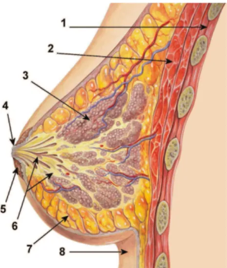
The breast (Figure 2.2) is a modified skin gland that lies on the chest wall, usually between the clavicle and the sixth rib, and is bounded externally by skin and in-ternally by the pectoralis muscle. Breast tissue also extends up into the axilla via

(23)

a pyramidal-shaped axillary tail. The breast tissue primarily consists of a combi-nation of fat and glandular tissue, with the relative proportions of the two varying widely. The remainder of the breast is made up of connective tissue, vascular tissue, lymphatics, and nerves.

Figure 2.2: Anatomy of the Breast: 1. Chest wall 2. Pectoralis muscles 3. Lobules 4. Nipple 5. Areola 6. Ducts 7. Fatty tissue 8. Skin.

Skin and Connective Tissue

The breast is supported by a combination of connective tissue and skin, whose thick-ness varies between 0.8mm and 3mm. The skin also contains the nipple, which is slightly below the centerpoint of the breast and extends about 5-10mm above the skin surface, and the surrounding areola, which contains small bumps called Mont-gomery’s glands. Finally, the breast is supported by a surrounding layer of connective tissues, which is interspersed with the subcutaneous and retromammary adipose tis-sue, and suspensory ligaments that provide an internal supporting framework for the breast lobes.

Adipose Tissue

The adipose tissue in the breast can be divided into three main groups: subcutaneous, retromammary, and intraglandular. The first two regions form a layer between the majority of the glandular tissue and the external boundaries of the breast. The majority of cancers develop in the region of glandular tissue within 1 cm of these fat layers.

(24)

Glandular Tissue

The glandular tissue in the breast consists of a number of discrete lobes, which are made up of lobules and ducts. There are approximately 15-20 lobes in each breast, and each lobe is thought to be exclusively drained by its own individual duct system. Within a lobe there are dozens of lobules 2-3 mm in diameter, and within each lobule there are as many as 100 alveoli, which are the basic secretory units of the breast.

Other tissues are present inside human breast, like Vascular, Nerve and Lymphatic tissues, which respectively provide blood supply, receptors and lymph fluid drainage.

2.3 Electrical Properties of Human Breast Tissue

Large differences exist in dielectric properties of biological materials. These differ-ences are determined, to a large extent, by the fluid content of the material. For example, blood and brain conduct electric current relatively well. Lungs, skin, fat and bone are relatively poor conductors. Liver, spleen, and muscle are intermedi-ate in their conductivities. In this section, the dielectric properties of human breast tissues will be discussed in order to explain the principles of microwave imaging [19]. In Microwave Imaging the dielectric properties are reconstructed regarding the differences in the complex permittivity, while non-metallic materials are considered in biomedical applications, defined by Equation 2.5:

"r = "0 j"00 (2.5)

where j = p 1 is imaginary unit, "0 describes the polarization eﬀects of charged particles in the tissue and "00 describes the out-of-phase losses due to the displacement currents generated by the applied electromagnetic field. Considering the biological tissues as dielectrics, the losses often are described by the conductivity , which is approximated to the displacement current eﬀect only, as Equation 2.6:

= 2⇡⌫"0"00 (2.6)

where "0 = 10

9

36⇡ F

m is the permittivity of free space and ⌫ is the frequency. The

dielectric properties are determined as "0 and "00, or "0 and , "r = "0 j

2⇡⌫"0 (2.7)

(25)

In the microwave region the dominant relaxation is the dipolar relaxation of polar molecules (i.e. water and many proteins). Therefore, the dielectric properties of the tissues in microwave region are highly correlated to the water content. Permanent dipoles of polar biological molecules are randomly oriented, but if an external electric field is applied, they will reorient statistically and the induced dipoles will follow the direction of the applied field. The rotational force exerted by the field on a permanent dipole is defined by the torque:

~

M = q~L_{⇥ ~}E (2.8) where q is the charge, ~L is charge separation, and ~E is the electric field strength. The rotation of polar molecules in an applied electric field requires time, hence, causes a dispersion occurs. Equation 2.9 is valid for this kind of dispersion and it describes any one-time constant relaxation mechanism. However, a distribution of time constants will often be found due to molecular inhomogeneity and nonspherical shape. The time constant is proportional to the cube of the radius of the molecules, and typical characteristic frequencies are, e.g., 15-20 GHz for water and 400-500 MHz for simple amino acids. Proteins add another dispersion typically centered in the 1-10 MHz range [20].

Gabriel et al. [21, 22, 23, 24] made a major review of measured dielectric properties together with own measurements on healthy human tissues, in order to physical model human tissues for frequencies between 10 Hz–10 GHz. They showed that relative dielectric permittivity and conductivity of high-water-content tissues (i.e., muscle and malignant tumors) are about an order of magnitude greater than those of low-water-content tissues (i.e., fat and normal breast tissue). In Figure 2.3, it is shown the comparison of the conductivity of high-water-content tissue with low-water-content tissue. In both cases conductivity and relative permittivity were greater in malignant tissue than in normal tissue of the same type, especially at frequencies below 1 GHz. This suggests that microwave imaging is theoretically possible at many frequencies, and that the choice of frequency is largely a matter of balancing the added spatial resolution aﬀorded by higher frequencies with the additional attenuation that comes with it.

(26)

Figure 2.3: Comparison of permittivity and conductivity of high-water-content tissue with low-water-content tissue as a function of frequency [21, 22, 23, 24].

The basic model is the Debye expression in Equation 2.9: "r = "1+

"

1 + j2⇡⌫⌧ j2⇡⌫"0 (2.9)

where " = "s "1, ⌧ is the time constant of the relaxation mechanism, "1 is

the permittivity at frequencies 2⇡⌫⌧ 1, "s the permittivity at 2⇡⌫⌧ ⌧ 1.

Figure 2.4 shows the fit of dielectric properties of normal and cancerous tissues exploiting Debye model, over a spread frequency spectrum.

Figure 2.4: Single-pole Debye curve fits of measured baseline dielectric properties data for normal and malignant breast tissue at radio and microwave frequencies [16]. Due to the complexity of the structure and composition of biological tissues, Lazebnik et al. [25, 26] performed a large scale study in order to experimentally

(27)

characterize the dielectric properties of a significant number of normal breast tissues and malignant tissues, from 0.5 to 20 GHz. The study of distributions of sample tissue compositions demonstrates that the dielectric properties of breast tissue are primarily determined by the adipose content of the tissue sample (Figure 2.5). Furthermore, secondary factors such as patient age, tissue temperature and time between excision and measurement had only negligible eﬀects on the observed dielectric properties. Also, the dielectric constant and eﬀective conductivity values for normal breast tissue reported in this study span a much larger range than those reported in most of previous smaller-scale studies. In contrast with normal tissue, the dielectric properties of malignant tissues are high and span a relatively small range.

Figure 2.5: One-pole Cole–Cole fits to the 85 normal data sets. The curves are color coded based on the amount of adipose tissue present in each sample. The solid black (upper) curve represents the dielectric properties of saline, the dashed black (lower) curve represents the dielectric properties of lipids, and the dash-dot black (middle) curve represents the dielectric properties of blood. [26]

In addition, Lazebnik et al. found the dielectric properties for the groups: low adipose tissue content (0-30%), median adipose (31-84%), high adipose (85-100%), and cancer tissue. Dielectric constant and eﬀective conductivity dispersion curves (Figures 2.6) are obtained for each group by fitting the data with single pole Cole-Cole model:

"r = "1+

"

1 + (j2⇡⌫⌧ )1 ↵ + j_2⇡⌫"

0 (2.10)

The Cole-Cole Model oﬀers an eﬃcient and accurate representation of many types of biological tissues over a very wide frequency band and has been used to reduce the complexity of the experimental data obtained for various human breast tissues (brain, fat, breast, skin, bone, etc.) .

(28)

Figure 2.6: Comparison of data obtained from single-pole Debye curve fits with previous studies. Lines: median dielectric properties of the cancer samples with 30% or greater malignant tissue content. Vertical arrows: range of data reported by Campbell and Land (1992) at 3.2 GHz for malignant tissues. [26]

Median dielectric constant and eﬀective conductivity dispersion curves were ob-tained for each group by first calculating the fitted values for each sample in the group at 50 equally spaced frequency points. Second, the median value at each fre-quency point was calculated across samples within the group. Finally, the Cole–Cole model was fit to these median values. The resulting ‘median curves’ fit the median values very well in all cases (Figure 2.7). In order to ensure that no systematic bias was present in the dielectric-properties characterization of the normal tissue samples obtained from cancer surgeries, these curves were compared with the curves obtained in the same manner from breast reduction surgeries.

(29)

Figure 2.7: Comparison of median Cole–Cole curves for normal and malignant tis-sue with measured dielectric properties of tistis-sue-mimicking phantom materials ([27]). (a) and (b) Dielectric constant and eﬀective conductivity, respectively, for the three adipose-defined normal tissue groups. Solid lines: median Cole–Cole curves for nor-mal tissue samples obtained from cancer surgeries (in the order of highest to lowest dielectric properties: group 1, group 2 and group 3). Dashed lines: median Cole–Cole curves for group 2 for normal tissue samples obtained from reduction surgeries. (c) and (d) Median Cole–Cole curves for the dielectric constant and eﬀective conductiv-ity, respectively, of cancer samples with minimum malignant tissue content of 30%. Symbols: measured dielectric properties of TM phantom materials (∗, 10% oil; , 30% oil; /, 50% oil; , 80% oil). [26]

They concluded that the contrast in the microwave-frequency dielectric properties between malignant and normal adipose-dominated tissues in the breast is consider-able, as large as 10:1, while the contrast in the microwave-frequency dielectric prop-erties between malignant and normal glandular/fibroconnective tissues in the breast is no more than about 10% (Table 2.1).

(30)

"₁ 4" ⌧(ps) ↵ S(S/m) Maximum 1.000 66.31 7.585 0.063 1.370 Glandular-high 6.151 48.26 10.26 0.049 0.809 Glandular-median 7.821 41.48 10.66 0.047 0.713 Glandular-low 9.941 26.60 10.90 0.003 0.462 Fat-high 4.031 3.654 14.12 0.055 0.083 Fat-median 3.140 1.708 14.65 0.061 0.036 Fat-low 2.908 1.200 16.88 0.069 0.020 Minimum 2.293 0.141 16.40 0.251 0.002 Malignant 9.058 51.31 10.84 0.022 0.889

Table 2.1: Single-Pole Cole–Cole parameters for normal [28] and malignant tissue [29] over the frequency band (3–10) GHz.

2.4 State of Art of MWI prototypes

Over the last decads, diﬀerent prototipe systems for microwave imaging have been developed by various research groups. These systems are conceptually simple and can be divided in three main parts:

· An antenna array, which consists of a set of antennas properly arranged to be in contact directly with the breast or through a coupling liquid;

· Front-end circuits for generating and acquiring microwave signals. Between antennas and front-end circuits a switch matrix is connected, that allows indi-vidual activation of antennas;

· Back-end processing system for image reconstruction.

In many cases, the antennas have been developed and customized for the specific application, whereas the switch matrix and the front-end electronics use commer-cial components and a Vector Network Analyzer (VNA). In none of the cases cus-tom integrated circuits have been developed for the specific application, even though the advancement of CMOS technology would permit nowadays to build those high-frequency components, to integrate them in order to reduce the bill of materials, and to simplify the connection between the antennas and the front-end. As for the back-end, a personal computer has been used, even if the reconstruction algorithms need high calculation capacity. This choice is allowed because most of the studies concern research prototypes, often tested with phantoms, in which processing performance is not the main goal.

(31)

The first MWI system for breast cancer detection (Figure 2.8) appeared in 2000 and was the first used in clinical environments [30]. That system was the precursor of various MWI systems developed in the following years. A significant limitation in dealing with microwave signals is the dynamic range needed to reliably acquire the weak signal originated by the tumor. This dynamic range is almost 100-120 dB, and it was quite diﬃcult to achieve several years ago with commercial VNAs. This is one of the reasons why in the Dartmouth prototype the VNA was replaced by ad-hoc designed circuits, yet still using commercially available components [30]. Moreover, the crosstalk between diﬀerent channels is another key parameter. An isolation of 100 dB is mandatory and it seems doable nowadays with commercial VNAs.

After this first prototype, various research groups built their own prototypes, which are listed here and some of them are presented in the following sections:

· Dartmouth college (USA) · Politecnico di Torino (Italy) · Chalmers University (Sweden) · University of Bristol (UK)

· Technical University of Denmark (Denmark) · University of Calgary (Canada)

· Shizuoka University (Japan)

· Electronics and Telecommunications Research Institute (ETRI, South Korea) · University of Lisboa (Portugal).

Despite the great deal of work that has been done on microwave breast cancer imag-ing, most of the methods mentioned above have been mainly checked against synthetic data or under controlled laboratory conditions. In the first case numerical breast models of increasing complexity as the research progressed have been used. Now, breast models are directly derived from MR images. In the second case, laboratory phantom, 2D and 3D, mimicking the breast tissues have been used in laboratory.

(32)

2.4.1 Dartmouth College

This clinical prototype was the first prototype for microwave imaging breast anal-ysis ever developed [30]. It provided useful information on the dielectric properties of breast tissues. From a technical point of view, the electronics circuits used were relatively old (it was the year 2000), but the building of such a system was quite an achievement. The system was developed to work at relatively low frequencies (300MHz-1GHz) and used an antenna array, front end electronics placed under the patient bed, and a PC for elaborating and visualizing the image. The analysis em-ployed a tomographic technique.

(a) (b)

(c)

Figure 2.8: Diﬀerent parts of the first MWI developed at Dartmouth College: (a) front-end electronics, (b) gurney and (c) antennas array.

16 vertical monopole antennas were used. Antennas protruded through the middle of the tank, with the radiating elements surrounding the breast on a 15-cm diameter. Each antenna was designed to work both as receiver and transmitter, maximizing the circuit flexibility. The liquid used as interface inside the tank was a saline solution. The antenna array and the tank are placed on a cart to be easily moved under the patient bed. The antenna array was connected with the front-end electronics (Figure 2.8a). The front-end was based on a heterodyne receiver, a 200-kHz A/D board, a function generator, a microwave source, while signal phase and amplitude extraction were performed in software with a Dell 300-MHz PC. The system was designed to

(33)

support up to 32 antennas through an electronic switch matrix that provides isolation greater than 120 dB and an overall linear dynamic range of 130 dB. An HP85070B Dielectric Probe Kit in conjunction with an HP 8753C Network Analyzer and a Dell Dimension 466V PC were used instead for system calibration. The whole system was placed on its own cart located under the patient bed.

The system was improved in 2005 (Meaney et al. 2005). The modulation scheme was again based on a superheterodyne approach and the frequency range was in-creased to 500MHz-3GHz. The radiofrequency signal was modulated and sent through an electronic switch matrix to 16 antennas. The same radiofrequency signal without modulation was sent to 16 transceiver boards through power dividers. The illumi-nation tank and the antenna array were similar to the previous prototype. Signals generated by each transceiver were sampled by a National Instruments data acqui-sition board, and sent to a PC for image visualization. When the board works in transmitter mode, the modulated radiofrequency signal is sent directly to the an-tenna. When it works in receiver mode the signal received by the antenna is sent to the mixer for being demodulated.

Using this device and further improvements, 80 patients with abnormal mam-mograms and 50 patients with normal mammam-mograms have been considered. The electrical permittivity and conductivity in the region of interest (ROI), the region which was suspicious in the mammogram, were reconstructed using the measured microwave data. The electrical permittivity and conductivity in the ROI were then compared to the background permittivity and conductivity outside the ROI in the ipsilateral breast (the breast with the suspicious legion) and to the mirrored ROI in the contralateral breast (the other breast). In the normal patients pseudo-ROI were selected. The results showed that cancerous tumors more than 1 cm in diameter exhibited twice as large conductivity in comparison to the background tissue. This ratio was statistically larger than that of benign tumors or that exhibited by healthy patients.

2.4.2 Politecnico di Torino - LACE Prototype

The microwave imaging system developed by LACE group of Politecnico di Torino is composed of the following parts:

· VNA

(34)

· Antenna array

This prototype uses 8 antennas (Figure 2.9a) interfaced with the breast through a tank (Figure 2.9b) containing a liquid used to reduce the unwanted reflections from the tank walls. In this prototype (which was not meant for clinical use) alcohol has been used as coupling liquid because of its optimal properties (from a microwave point of view): the return loss measured for the used antenna is below -10 dB from 0.5 GHz up to 5 GHz. Thinking to a clinical application, this is not the best choice. A possible mixture could be a bath composed of glycerin and water in diﬀerent proportions. This liquid is not hazardous for the patient, and provides a good mechanical contact. The antenna (Figure 2.9c) is a simple monopole designed to work immersed in a liquid. It exhibits wideband behavior from few hundreds of MHz up to few GHz. A multi input VNA is used to generate and acquire microwave signals.

(a) (b)

(c)

Figure 2.9: PoliTo-LACE prototype: (a) antenna array, (b) array with liquid tank and (c) monopole antenna.

2.4.3 Technical University of Denmark

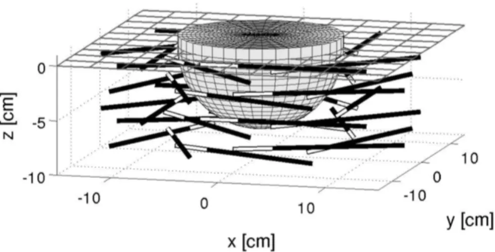
This prototype for microwave imaging developed at Technical University of Denmark is based on a 3D nonlinear inverse scattering algorithm. The antenna array is made of 32 horizontally aligned monopole antennas (Figure 2.11b) in a cylindrical setup with a radius of 8 cm. Antennas are organized in a 3D volume to provide a 3-dimensional picture of the breast (Figure 2.10). These antennas are immersed in a tank filled with a glycerin-water mixture.

(35)

Figure 2.10: Antennas position in the prototype developed at the Technical University of Denmark.

The system works between 500 MHz and 3 GHz and each antenna operates both as transmitter and receiver. The electronics front-end uses instead custom electron-ics. Every antenna is connected to its own transceiver module (Figure 2.11a). The transceiver contains a low noise amplifier and a radiofrequency amplifier. The signal received from the antenna is amplified and then mixed with the local oscillator signal. A value of 1 KHz is chosen as intermediate frequency. The signals generated by the transceiver modules are then fed to 18-bit Analog-To-Digital (ADC) converters with built in 10 KHz low pass filters. The total measurement time with this set up is 2 minutes for each breast.

(a) (b)

Figure 2.11: (a) Antenna array, tank and transceiver modules; (b) Detail of a monopole antenna.

(36)

agree-ment with the images obtained by X-ray mammography for certain patients.

2.4.4 University of Lisboa

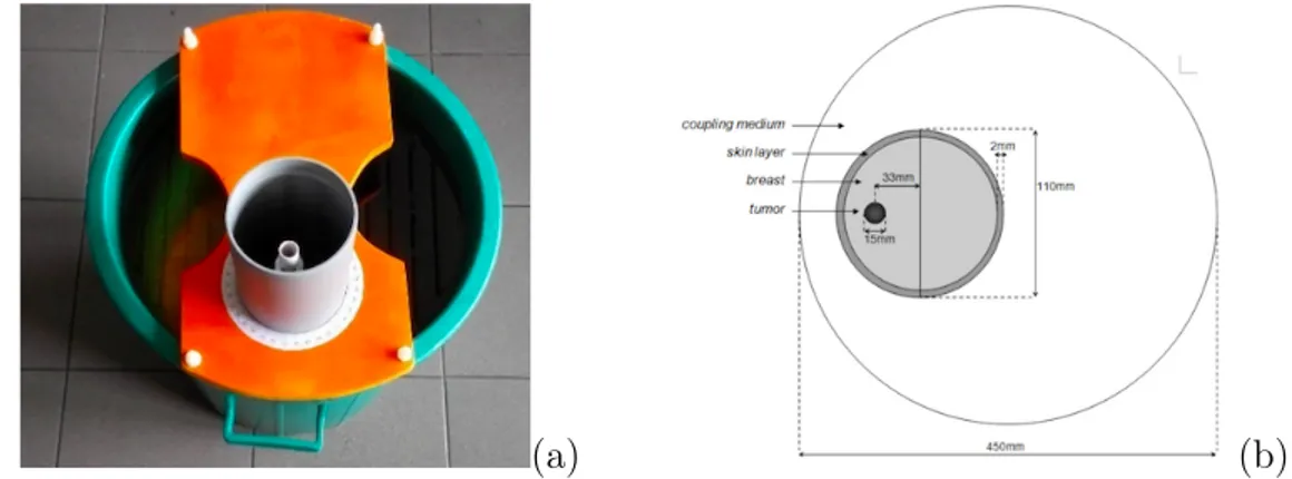
University of Lisboa realized a tumor classification exploiting a pre-clinical UWB prototype imaging system developed at the University of Manitoba (Canada). The system is composed of a Field Fox N9923A VNA by Agilent Technology, a Vivaldi antenna which is connected to the VNA through a 50-ohm cable and is attached to the inner part of a Plexiglas tank filled with canola oil (Figure 2.12).

Figure 2.12: Microwave system developed at the University of Manitoba. The breast phantom consists of a styrene-acrylonitril cylinder with a diameter of 13 cm and an height of 35 cm filled with glycerin, while the tumor phantoms were emulated with a mix of TX151 solidifying powder and water. A set of 13 benign and 13 malignant tumors (Figure 2.13) with a diameter ranging from 13 mm to 40 mm were considered for the classification. Spiculated and microlobulated shapes emulate the malignant tumors, while the spheres represent the benign tumors.

Figure 2.13: Tumor phantoms.

During the experimental acquisitions, a monostatic radar system was considered, thus the VNA worked as both microwave waveform generator and receiver for the reflected waves. The frequency was swept from 1 to 6 GHz for each tumor model

(37)

and at 144 diﬀerent angular positions. The results of benign and malignant tumor classification was performed through a further post-processing of the acquired data, based on the Radar Target Signature (RTS) of the tumors. The results are in good agreement with simulations.

(38)

Chapter 3 Reconstruction Algorithm

Microwave imaging is a technique aimed at investigate a given domain by means of microwaves and reconstruct the scattering scenario, starting from the equations that govern electromagnetic scattering phenomena. Several approaches can be ap-plied to localize, shape and reconstruct an unknowkn target located in the area of interest, surrounded by an arbitrary number of measurement probes able to acquire the samples of the scattered field. Those considered in this thesis are inverse scat-tering procedures. Inverse scatscat-tering is an ill-posed problem (i.e., small variations in the measured data can lead to large errors in the reconstructions), whose solution is achieved through Time-Reversal Imaging (TR). The scatterer is localized by MUlti-ple SIgnal Classification algorithm (MUSIC)[31]. This method, called TR-MUSIC, has been developed by Devaney [39, 44, 45].

In this work a Multi-frequency approach is exploited. Data collected at diﬀerent frequencies through a Vector Network Analyzer are employed to overtake limits of the single-frequency case and combined in MUSIC-like methods.

In order to obtain an image of the domain under test, it is conventient to accom-plish a pre-processing analysis of the measured data that consists in:

· Clutter mitigation: the reflections due to the skin layer and internal antenna reverberations produce raw data in which clutter is diﬀerent orders of magnitude greater than the signal corresponding to the scatterers. In order to clean the data from these useless contributions the low frequency content is filtered out (i.e., the average component is subtracted from the data)

· Preliminary assessment of scattering scenario: in this step, mean value for Debye parameters are estimated to reduce blurring in the detection procedure · Reconstruction algorithm (§3.3)

(39)

· Evaluation of the reconstruction through the study of spatial and contrast fea-tures (§3.4)

3.1 Basic Ideas in Direct and Inverse Scattering

Scattering theory, in the time dependent formulation, is the study of the long time be-haviour of solutions of an evolution equation that move out to infinity. The evolution equation might be the time dependent Schrödinger equation (quantum scattering), the scalar wave equation (acoustical scattering), Maxwell’s equations (electromag-netic scattering) or even a non-linear evolution equation. The underlying space might be Euclidean space or a Riemannian manifold. In each problem there is a localized scattering target. Moving in space away from the target to infinity, the equations, or the geometry, become simpler. The idea is that in the distant past and in the far future, the scattered wave will be located in the region where the equation or geometry is simple. It then becomes possible to compare distant past input to the far future output. Inverse scattering is how we obtain a large part of our information about the world. Form a physical point of view, it is generally recognized that the diﬀerences between direct and inverse problems are related to the concepts of cause and eﬀect. By the way, it is arbitrary to define whether a problem is the direct or inverse part respect to its counterpart, since one generally calls two problems inverse to each other if the formulation of one problem involves the other one, and the direct problem is usually referred to the simpler one or the one which was studied earlier [32].

The inverse scattering problem considered here belongs to the category of inverse problems. An everyday example is human vision: from the measurements of scattered light that reaches our retinas, our brains construct a detailed three-dimensional map of the world around us. Our knowledge about interior structure of the Earth is given by the solution of the inverse problem of determining the sound speed by measuring travel times of seismic waves. Many other cases exist in diﬀerent areas of nature (the way dolphins construct a detailed three-dimensional map of the world around them, etc.), science (the investigation of the DNA structure solving X-ray diﬀraction problems, etc.) and industry (non-destructive evaluation of materials to find cracks and corrosions, oil exploration, etc.). Medical imaging uses scattering of X-rays, ultrasound waves and electromagnetic waves to make images of the human body which is of invaluable help with medical diagnosis.

(40)

Kx = y

where K is an operator mapping elements of the normed space X into elements of the normed space Y . The problem turns out to be well posed if the operator K is bijective and the inverse operator K 1 _{is continuous, so that the solution depends}

continuously on the data and the stability is guaranteed.

Figure 3.1: If a problem is ill-posed, small variations on the data (4x) produce big variations on the solution (4y), such that |4x|  c|4y|, c 1.

The most critical aspect of an inverse problem is usually its ill-posedness. Accord-ing to Hadamard’s definition, a problem is well posed if its solution exists, depends continuosly on the data and is unique, so that a small perturbation of tha data results in a small perturbation of the solution. If one of the previous condition is not satified, the problem is called ill-posed or improperly-posed (Figure 3.1). In orer to make the solution of ill-posed problems more stable, regularization methods may be applied. Theis aim is to find a tradeoﬀ between accuracy and stability of the solution exploit-ing additional a-priori information which reduces the instability of the solution at the price of finding an approximate version of it [18].

In imaging applications, we obtain information on the object subjected to the incident radiation starting from the measurements of the scattered field, and the ill posedness may lead to different scenarios. If two or more different objects produce the same measured data, the solution of the problem is not unique. Moreover, if two significantly different objects produces very similar set of measurements, the problem solution does not dipend continuosly on the data, since small measurement errors result in large errors in the solution. The information exploited to obtain a more stable solution regards the knowledge of some physical features of the target to be detected or the noise level of measured data.

(41)

be-tween the input and output waves, given the details about the physical laws and the scattering target. On the other hand, the aim of inverse scattering theory is to de-termine properties of the target from future observations through the calculation of the evolution of the system backwards in time, given suﬃciently many input-output pairs. In fact, most often scattering problems are stated in a time independent for-mulation that results after taking a Fourier transform in the time variable. Although the immediate connection to the original scattering experiments is obscured, it can be easier to state and study scattering problems in this formulation.

3.2 Inverse Scattering Problem

3.2.1 Linear Inverse Scattering

The imaging problem for point targets can be roughly defined to be that of forming an “image” of the distribution of target scattering centers from measurements of the fields generated in a suite of N scattering experiments that employ the set of incident fields inc_{. The goal of inverse scattering problem is the quantitative determination of}

both the target positions and the target scattering strengths ⌧m, m = 1, . . . , M, from

the available scattered field data. It is assumed that one knows the background Green function G0(r, r0)of the medium in which the targets are embedded. The background

medium can also be heterogeneous with possible sharp boundaries and reflecting surfaces. The inverse scattering problem consists in deducing the target positions and scattering strengths from knowledge of the full Green function specified at all transmitter/receiver pairs as well as of the background Green function at all pairs of points (r, r0₎ _{within the background medium [33]. This semplified model is able to}

produce only qualitative informations, thus a further classification step is generally needed. From a pratical point of view, problems of reliability and computational burden are avoided.

In the last two decades, diﬀerent linear inversion techniques have been developed and applied in breast cancer detection field.

The classical time-domain techniques to solve linear inversion problems belong to beamforming methods framework, in which diﬀerent approaches have been devel-oped. The simplest algorithm of this family, called Delay And Sum (DAS), provides the reconstructed image as a sum of the contribution obtained by delaying the regis-tered time-domain signals knowing the wave propagation speed in the space domain. Diﬀerent improvements of this method was carried out, such as Delay Multiply And

(42)

Sum (DMAS), Improved Delay And Sum (IDAS). O’Halloran et al. [34] proved that both the IDAS and DMAS significantly outperform the DAS beamformer where the breast is mainly composed of adiposetissue and is primarily dielectrically homoge-neous. However, in the more dense model, where fibroglandular tissue contributes to a significant mismatch between the assumed and actual channel propagation models, the improved performance promised by both IDAS [35] and DMAS is significantly reduced. Other approaches belonging to the beamforming family are the Microwave Imaging via Space-Time (MIST [36]) and Confocal Microwave Imaging (CMI [16]) beamforming techiques.

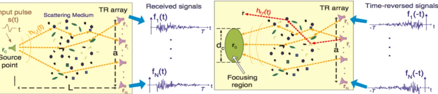
In addition to these methods, a Time-Reversal (TR) methods are based on the time reversibility of the wave equation in a stationary and lossless medium [37][40]. In TR imaging one or more unknown scatterers are sequentially probled using a set of N antennas and the backscattered returns are measured at all the antenna locations and involves physical or synthetic retransmission of signals acquired by a set of transceivers in a time-reversed fashion, i.e. last-in first-out. The retransmitted signals propagate “backwards”, naturally reversing the path that they underwent during forward propagation, which results in (automatic) energy focusing around initial source location (Figure 3.2). The “source” in this case can be either active or passive.[38].

Figure 3.2: A point source located at ¯r transmits a short Ultra Wide Band pulse s(t). (left) The transmitted signal propagates through the medium and is received by an antenna array (forward propagation). (right) The signals received at each array element are recorded, reversed in time, and transmitted back to the same medium.

The TR techniques that rely on ultrawideband (UWB) operation are further at-tractive because they can exploit advantages of simultaneous operation at low (e.g., more penetration into lossy materials) and high frequencies (e.g., better resolution), and because they enable imaging techniques in random media that depend only on the statistical properties (instead of a particular realization) of the random media,

(43)

i.e., they are statistically stable. Also, they allow to achieve superresolution, meaning that the resulting resolution beats the classical diﬀraction limit[38]. The most signif-icant development of TR algorithm are Decomposition of the TR Operator (DORT) and TR MUltiple Signal Classification (TR-MUSIC).

3.2.2 Non-Linear Inverse Scattering

The inverse problem is formalized by finding the unknown contrast distribution of the object from the measured scattered field at the receivers, for a known incident field, such as the dielectric and conductivity maps of the breast.

The non-linear inverse scattering problem may be solved by an iterative opti-mization process, where the difference between the measured field and the computed field from the direct problem is minimized. When the error is sufficient small the reconstructed image of the object is the complex permittivity map used in the di-rect problem. In these algorithms, the distribution of the constitutive parameters in the imaging domain is updated by steps. In each iteration, the scattered field from the current parameter distribution is calculated and compared with the measured field. This optimization process may be arranged in a Least Square formulation called Newton-Kantorovich [41], Levenberg-Marquardt [42] or Gauss-Newton algo-rithm [43]. These techniques require that the scattered field is calculated in each iteration using a forward solver, such as Finite Difference Time Domain (FDTD), Finite Element Method (FEM) or Method of Moments (MoM).

Forward solvers are heavy from a computational point of view. For this reason non-linear imaging algorithms are less applied than linear algorithm.

3.3 Time Reversal and MUSIC

3.3.1 The general approach

We consider an array of N antennas centered at the space point Rj, j = 1, 2, ..., N

not necessarily regularly spaced or belonging to a plane. Each antenna is assumed to radiate a scalar field j(r, !) in a domain D in wich are embedded one or more

targets. The antennas and the targets are respectively assumed to be monopoles (point antennas) and ideal point scatterers. Also, all multiple scattering between targets are neglected.

Under these simplifying assumptions, the wavefield radiated by the j-th antenna element and the resulting scattered field are equal to

(44)

inc j (r, !) = G(r, Rj, !)ej(!) (3.1) sc j (r, !) = M X m=1 G(r, Xm, !)⌧mj(!)G(Xm, Rj, !)ej(!) (3.2)

where M is the number of the targets, ! is the frequency, ⌧m(!) is the scattering

amplitude, Xm is the location of the m-th target, ⌧m(!)is the input voltage applied

at the terminals of the j-th antenna element, ej is the j-th antenna excitation voltage

and G(r, r0₎_{is the Green’s function of the background medium.}

When all antenna elements are simultaneously excited using the voltages ej(!)

the total incident scattered wavefields are given respectively by

inc_{(r, !) =} N X j=1 inc j (!) = N X j=1 G(r, Rj, !)ej(!) (3.3) sc_{(r, !) =} N X j=1 sc j (!) = N X j=1 M X m=1 G(r, Xm, !)⌧mj(!)G(Xm, Rj, !)ej(!) (3.4)

The voltage output vl(!) corresponding to l-th antenna is assumed to be equal to

the amplitude of the scattered field as measured at the l-th antenna ans is given by vl(!) = N X j=1 sc j (Rl, !) = N X j=1 M X m=1 G(Rl, Xm, !)⌧m(!)G(Xm, Rj, !)ej(!) (3.5)

Equation 3.5 can be expressed in a compact matrix notation as follows vl(!) =

N

X

j=1

Kl(!)ej(!) = K(!)e(!) (3.6)

where e(!) = [e1(!), e2(!), ..., eN(!)]T is the N-dim column vector formed from

the set of input voltages applied at the antenna terminals and K is named Multistatic Response Matrix (MSR). It represents the matrix propagator, whose (i,j) element stands for the total field received by the j-th element when i-th element is “fired”, ans is defined as follows

(45)

K(!) ={Kl,j(!)} = M X m=1 G(Rl, Xm, !)⌧m(!)G(Xm, Rj, !) = M X m=1 ⌧m(!)gm(!)gTm(!) (3.7) and gm(!) is the N-dim Green function column vectors:

gm(!) ={G(Rl, Xm, !)} = [G(R1, Xm, !), G(R2, Xm, !), ..., G(RN, Xm, !)]T

(3.8) The Green functions G(r, r0₎ _{are completely general since the above formulation}

applies to both homogeneous and non-homogeneous media. It is possible to define the correlation matrix, called Time Reversal Matrix (TRM), given by

T (!) = K†(!)K(!) = K⇤(!)K(!) (3.9) where K†_(!) _{and K}⇤_(!)_{are the Hermetian and the complex conjugate of K(!),}

respectively. The equality K†_{(!) = K}⇤_(!) _{holds because MSR is symmetric. From}

Equation 3.9 and Equation 3.7 we obtain the final result T (!) = [ M X m=1 ⌧m(!)gm(!)gTm(!)]⇤[ M X m=1 ⌧m(!)gm(!)gTm(!)] = M X m=1 M X m0₌₁ ⇤m,m0g⇤_m(!)gT_m0(!) (3.10) where ⇤m,m0 = ⌧_m⇤⌧_m0hg_m(!), g_m0(!)i (3.11)

and the angular brackets stand for the standard inner product in CN_.[39]

The TRM possesses a complete set of orthonormal eigenvectors corresponding to non-negative eigenvalues, because T (!) is Hermetian and non-negative. TRM eigenvectors correspond one-to-one with the diﬀerent targets, and if M  N, the rank of T (!) will be equal to M, so that there are exactly M non-zero eigenvalues.

The goal now is to estimate the locations of the targets from the measured scat-terer field data. One of the main approach emploied to reach this goal is the MUSIC algorithm , that is to be used in conjunction with time-reversal processing. We still will require multi-static data and the multi-static response matrix K(!) and will compute the time-reversal matrix T (!) = K⇤ _(!)K(!) _{and the eigenvalues and}

(46)

eigenvectors of this matrix. Through MUSIC algorithm it is possible to deal both with non-resolved targets as well as with sparse antenna arrays.

The MUSIC algorithm makes use of the fact that the time-reversal matrix T (!) is a projection operator onto the subspace of CN _{spanned by the complex conjugates of}

the Green’s function vectors (i.e. the signal subspace S) and that the noise subspace N is spanned by the eigenvectors of T (!) having zero eigenvalue, where CN ₌_{S N .}

It follows that the complex conjugte of each Green’s function vector is orthogonal to the noise subspace and, in particular, to the eigenvectors of TRM having zero eigenvalues:

hµm0(!), g⇤m(!)i = hµ⇤m0(!), gm(!)i = 0 (3.12)

for m = 1, 2, ..., M scatterers, N antennas and m0 = M + 1, ..., N eigenvectors

having zero eigenvalue, where µm0(!) are the eigenvectors of T (!) having zero

eigen-value.

Now it it possible to form a pseudo-spectrum through the following equation, that is the key equation of MUSIC algorithm for time-reversal imaging

(rk, !) = 1 |P [Ak(!)]|2 = _P 1 N m0=M +1hAk(!), µ⇤m0(!)i 2 (3.13)

where P [·] is the projection operator onto N , µm0 is the m0-th eigenvector of

T (!)having zero eigenvalue and

Ak(!) = Gk(!)⌧m(!)GTk(!) (3.14)

is the steering matrix, that is the MSR matrix in the trial points rk of domain

D and Gk(!) = [G(R1, rk, !), G(R2, rk, !), . . . , G(RN, rk, !)]T. The inner product

in Equation 3.13 will vanish in a deterministic way when rk is equal to the actual

location of one of the scatterers both for resolved and non-resolved targets, and this happens because the signal subspace is orthogonal to the noise subspace [39]. In other words, the pseudospectrum will show a theoretically infinite peak at each target location in a deterministic way.

The achievable performance can be equivalently and more conveniently studied by employing the projector over the signal subspace S, uising Q [·] instead of P [·] as follows [48]

(47)

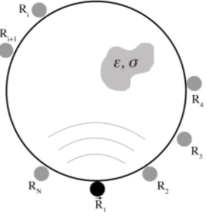
The acquisition system considered so far is called Multistatic configuration (Figure 3.3). In this configuration, the acquisition system is composed of N equidistant antennas positioned around the imaging domain, along a circumference. In each measure, an antenna trasmits and receives the signal from its position (Ri), whereas

the other N-1 antennas receive only. This operation is performed N times, once for each antenna.

Figure 3.3: In multistatic configuration an antenna trasmits and receives the signal and the other N-1 antennas receive only.

Multistatic apporach will not be explored in this work but a short description was given because it is the general case from which we can derive the equations for the approach used in this work, called monostatic configuration.

3.3.2 Monostatic configuration

In monostatic configuration, the acquisition system is composed of only one antenna, which acts both as trasmitter and receiver. This antenna rotates around the imaging domain and stops in diﬀerent equispaced positions R1, . . . , RN where the measures

are performed (Figure 3.4). Once the acquisition is completed, the antenna goes back in its original position.

(48)

Figure 3.4: In monostatic configuration the antenna moves in diﬀerent positions around the domain, from which it transmits and receives the signal from diﬀerent positions.

In this system configuration, we can semplify the description given in §3.3.1 thanks to the presence of only one antenna, indeed the response matrix K(!) reduces to a vector because the collected signal is always associated to the same antenna that produce the excitation pulse. The vector of voltage output from N antenna positions can be defined as

v(!) = [v1(!), v2(!), . . . , vN(!)] = K(!)e(!) (3.16)

where vl(!)is the voltage output from l-th antenna position derived from Equation

3.5 as follows vl(!) = scj (Rl, !) = M X m=1 G(Rl, Xm, (!))⌧m(!)G(Xm, Rl, (!))e(!) (3.17)

and K(!) = [K1(!), K2(!), . . . , KN(!)]T is the Monostatic Response vector (MoSR).

Now we can define the steering vector Ak(!) as MoSR calculated in the trial

points rk of domain D as follows

Ak(!) = [Ak1(!), Ak2(!), . . . , AkN(!)] (3.18)

whose elements are given by Equation 3.14. The goal of the imaging procedure is to detect the scattering source by finding the steering vector, that will produce the pseudospectrum peak because it is orthogonal to the noise subspace in rk.

Now, recalling Equation 3.15, it is possible to calculate the pseudo-spectrum as follows