Economic growth and balance-of-payments constraint in Vietnam

1

Economic growth and balance of

payments constraint in Vietnam

A. Bagnaia_{, A. Rieber}b_{, T.A.D. Tran}c

a _{Department of Economics, ‘Gabriele D’Annunzio’ University, Pescara, Italy}

b _{Department of Economics, University of Rouen, France}

c _{DIAL, Institute of Research for Development, Vietnam}

Our paper examines the long-run relation between economic growth and current account equilibrium in Vietnam, using a multi-country BoP-constrained growth model. We find that in the whole sample (1985-2010) Vietnam grew less than the rate predicted by the model. We also find that the BoP-constrained growth rate shifted after the 1997 Asian crisis. Since the relative price effect is neutral, the volume effects dominate in setting the BoP constraint. On the one side, owing to the high income elasticities of exports, growth in advanced countries has a strong multiplier effect on the Vietnamese economy. On the other side, this effect is hindered by a high ‘appetite’ for imports coming from Asia. Finally, we assess the impact of the current crisis on Vietnam’s growth for the period 2011 to 2017.

Keywords: Economic growth, BoP constrained growth model, Multi country model, Asia, Vietnam.

I. Introduction

The transition process from central planning to a market economy, launched in 1986 with Doi Moi

(‘renovation’ in Vietnamese), enabled Vietnam to shift in less than 20 years from one of the poorest

countries in the world (with per capita income of 98 USD in 1990) to a Lower Middle Income

(LMI) country (with per capita income of 1130 USD in 2010). Vietnam’s economy has grown at an

annual average rate of 7.3% from 1990 through 2010, outpacing other countries in the Asian region.

The ratio of population in absolute poverty has fallen from 58% in 1993 to 14.5% in 2008, while

most indicators of welfare have improved (World Bank, 2011).

Behind the story, integration in the world economy has been the key driver of Vietnam’s economic

and social development. The country has gone through a far reaching transformation from an

inward looking planned economy to one that is globalized and market-based. The country formally

completed World Trade Organization (WTO) accession in late 2006, culminating a long process of

efforts to integrate the national economy into global markets (Abbott et al., 2009). These changes

have had dramatic implications for trade and investment flows: exports and imports as a share of

Gross Domestic Product (GDP) increased tenfold from 1988 to 2008, reaching respectively 77.5%

and 87.8% of GDP in 2010. Over the last two decades, average growth rates of exports and imports

were 16.4% and 18% respectively, compared with 7.3% for GDP.

(Insert Figure 1 here)

However, owing to rapid growth and massive capital inflows, the country has experienced growing

macroeconomic turbulence in recent years. Between 2005 and 2007, the current account deficit

increased from 0.9% to 9.8% of GDP (Figure 1) while the capital account surplus increased even

faster, from 4.8% to 24.6% of GDP (World Bank, 2008). Net positive capital inflows have led to

demand pressures and subsequent changes in relative prices. Inflation rates averaged 16% a year

between 2008 and 2011, and asset price bubbles emerged, while the country was coping with

3

According to the World Bank (2011), the government addressed these macroeconomic imbalances

by relying almost exclusively on tight monetary policy, but it has yet to tackle their root causes.

From our point of view, the analysis of macroeconomic instability in Vietnam cannot be dissociated

from the country’s Balance of Payments (BoP) position. Substantial current account deficits and the

rising capital inflows to finance them played a significant role in perturbing macroeconomic

stability. Based on these stylised facts, the question naturally arises as to whether the country is

growing faster than the rate allowed by its BoP equilibrium.

To this purpose, our paper examines the long run relationship between economic growth and the

current account balance equilibrium using the BoP constrained growth model, originally developed

by Thirlwall (1979). While neoclassical theories explain growth through supply side elements such

as factor accumulation, technological progress or the contribution of productivity growth, this

alternative approach emphasises demand driven mechanisms, by postulating that in the long run

BoP equilibrium is the primary constraint on a country’s economic growth.

Our study aims at filling a number of gaps in the literature. From a theoretical point of view, the

analytical framework proposed here improves over previous attempts to extend Thirlwall’s law to a

multi-country setting (e.g., Nell, 2003), by allowing for a more rigorous disaggregation of the BoP

constraint among different partner areas (Bagnai et al., 2012). More precisely, our extended model

allows us to assess the relative importance of the different channels of transmission (real growth,

changes in relative prices and import/export market shares) in the different partner areas. From an

empirical point of view, the paper provides fresh evidence on growth performance in Vietnam since

Doi Moi, using annual data from 1985 to 2010. There have been several studies applying the BoP

constrained growth model to individual countries and groups of countries (Thirlwall, 2012), but to

our knowledge, no empirical study has yet tested the model for Vietnam; neither has there been an

analysis of long-run growth since the country’s accession to the WTO.

The paper is structured as follows. Section 2 presents the BoP-constrained growth model and the

and interprets our empirical results. Considering the recent global slowdown, Section 5 presents

some simulation exercises aimed at forecasting the impact of external shocks on Vietnam’s future

growth. Section 6 summarizes our main results.

II. The theoretical background

Thirlwall’s Law and the developing countries

According to Thirlwall (1979), the need to satisfy the external constraint in the long run sets an

upper limit to growth. Thirlwall's Law is expressed in these terms: ‘In the long run, no country can grow faster than the rate consistent with its balance of payments equilibrium on the current account, unless it can finance an ever growing external deficit, which, in general, it cannot’. In

other words, there is a growth rate that a country cannot exceed for prolonged periods, because if it

does, it will quickly incur into BoP difficulties. This is the ‘BoP-constrained growth rate’. Exports

play a major role in the definition of the BoP-constrained growth rate, because, in contrast to the

other components of aggregate demand, they are the only component whose expansion provides the

foreign exchange needed to pay for the import requirements associated with the following

expansion of output (Hussain, 1999).

Assuming constancy of relative prices, Thirlwall’s Law postulates that the rate of growth of an open

economy which is consistent with BoP equilibrium (denoted here Y ) is determined by the growth _BP

rate of its volume of exports ( ̇ ) divided by the income elasticity of imports (. To put it

differently, the BoP equilibrium growth rate depends on the growth of world income ( ̇) and on the

relative size of the income elasticities of demand for exports (and imports. This relation can be

formulated as follows:1   Z X Y_BP    _{  (1)}

1 _{Alternatively, Equation (1) can be obtained by assuming that the Marshall-Lerner condition is satisfied with}

5

If a country’s growth rate is lower thanY , the country will accumulate trade surpluses and become _BP

a net capital exporter. Conversely, if its actual growth exceedsY , the current account worsens and _BP

the country will become a net capital importer, but this cannot continue indefinitely. An economy is

‘BoP-constrained’ whenever its growth rate must adjust downwards to maintain the BoP equilibrium.

Two remarks are worth emphasising at this stage. Firstly, the model assumes that developing

countries operate at less than full capacity, as a result of the lack of foreign exchange and other

structural bottlenecks. However, although it stresses the role of growth in aggregate demand to raise

capacity utilisation, the model does not imply that supply factors are unimportant. Rather, any

production bottleneck that restricts export growth will be detrimental for growth (Felipe et al., 2009).

Secondly, this approach provides a rationale for an export-led growth model, because exports are

the only one component of demand whose growth simultaneously relaxes the BoP constraint.

Therefore, policies designed to increase the income elasticity of export (such as changing

composition of exports, or other measures that improve the performance of exports, may have

positive effects on long-run growth. But these efforts could be hindered by the country’s ‘appetite’

for imports (), that is by its degree of dependence on foreign goods and services. This implies that

the same rates of export growth in different countries do not produce the same rates of economic

growth, because of the existence of different income elasticities of imports.

Our study extends the original BoP-constrained growth model in two ways. First, we relax the

hypothesis of relative price constancy in Equation (1), which is contradicted by the evidence that in

developing countries the terms of trade are trending, as implied by the Prebisch-Singer hypothesis

(Sapsford and Chen, 1998). Such relative price changes appear to be relevant in a transition

economy like Vietnam, where the abolition of price and exchange rate controls in 1987, followed

by international integration, caused substantial adjustments in relative prices. Therefore, we decided

Our second extension deals with the geographical structure of trade flows. In the original model, the

long–run economic growth of an open economy is determined by the rate of growth of aggregate

exports, which is, in turn, determined by the exogenously given growth of ‘world income’. In

practice however, an individual country trades goods and services with a number of partner

countries, and each bilateral trade relations may have different outcomes. Since the economic

growth of a country depends on the growth rate of other countries through the BoP constraint, this

mutual interdependence should be captured in a model with multilateral trade relations between the

individual country and blocks of countries. By the same token, the import behaviour should be

differentiated among the selling countries to assess how geography can be a determinant of trade

relations. In view of this, we extend the original Thirlwall’s law by applying it in a multi-country

setting. This allows us to identify the role of structural parameters such as the imports and exports

market shares and the bilateral trade elasticities in determining the BoP-constrained rate.

A multi country version of Thirlwall’s Law

Our analytical extension assumes that a given country i has n trading partners. In our empirical

analysis, we set n = 5 by considering five main partner areas: j = A, B, C, D, E (see Appendix A for

country grouping). The current account equilibrium becomes: 2





where Pi are country i export prices, Xij is the real demand of partner j for country i exports, Eij is

the bilateral nominal exchange rate, Pj are export prices in j, and Mij are country i imports from

partner j. As a matter of fact, Xij = Mji (namely, the exports from country i to partner j must equal

the imports of the latter from the former). This ‘mirror flows’ identity, routinely exploited as a

convenient simplification in a number of multi-country models, offers some practical advantages in

terms of data collection and of the specification of the demand functions. Notably, it enables us to

work only with import functions.

7

As a consequence, we formulate the model as follows:

ij ij i j ij i ij Y P E P M            (2) ji ji j i j ij ji Y P P E M            (3)





Where, in addition to the previous variables, ij and ij are respectively the price and income

elasticities of country i imports from partner j, Mji is the real demand of partner j for imports from

country i (namely, exports from country i to partner j), ji and ji are the corresponding price and

income elasticities, and Yj is partner j real GDP.

Taking the growth rates in (4) we obtain:













ji and ij are respectively the market shares of partner j in country i total exports (in volume) and in

country i total imports (in value).3

Solving for the growth rate of country i as before, and denoting Rij = Pi/(EijPj) the bilateral relative

prices (namely, the ratio of domestic to foreign prices expressed in domestic currency), we obtain a

multi-country version of Thirlwall’s Law:















3 _{This asymmetric treatment of the market shares is a mathematical consequence of the fact that the summation}

in the left-hand side of the constraint (4) involves terms in volume, while the summation in the right-hand side involves terms in value.

The multi-country specification allows us to separately assess the contribution of each group of

countries to country i growth rate predicted by the model. We can observe that the numerator of the

multi country law features both a relative price effect (whose sign depends on the market shares

weighted bilateral price elasticities), and a volume effect (a weighted sum of real export growth).

The denominator instead features a sum of bilateral income elasticities of imports, weighted by the

corresponding market shares, that expresses country’s i aggregate ‘appetite for imports’





jijij

 . In other words, the aggregate income elasticity, that plays a crucial role in the single

country version of Thirlwall’s law, is nothing but a ‘black box’ summarising behavioural

parameters that are likely be subject to changes.

Another important feature of the multi-country law is that it cannot be decomposed in bilateral

terms. In fact, any bilateral deficit is not constrained per se, since in principle it could be financed

by another bilateral surplus; as a consequence, the aggregate BoP constraint cannot be expressed as

an additive function of bilateral balances. However, the extended law allows one to measure the

contribution of partner j’s variables (either in country i export market or import demand) to changes

in the aggregate BoP constraint of country i (see Bagnai et al., 2012).

III. Data and estimation issues

In a first step, the long-run elasticities featuring the BoP constraint are estimated through the

following ten loglinear bilateral trade equations:

mj,t = j + i,j rj,t + i,j yi,t + uj,t (j = A,B,C,D,E)

xj,t = j  j,i rj,t + j,i yj,t + ej,t (j = A,B,C,D,E)

Where lower case letters indicate natural logs of the corresponding variables (therefore, rj,t = pi,t –

ei,j,t – pj,t), and uj,t and ej,t are error terms.

Appendix B provides the sources and definitions of the data used in the estimation. In order to

9

Generating Process (DGP) of each series features a stochastic trend. The relevant tests were

performed following the procedure suggested by Elder and Kennedy (2001). The rationale of this

procedure is reported in Appendix C, along with its results. Summing up, all the time series

involved in the estimation of the trade equations for Vietnam turn out to possess a unit root.

Having established the presence of stochastic trends in the DGP of our time series, we tested for the

existence of a long-run relation between the relevant variables by the usual Engle and Granger

(1987) cointegrating residual ADF (CRADF) test. When this test rejected the null of non

cointegration, we took the estimated elasticities as the relevant long-run parameters. If instead the

ordinary cointegration test failed to reject the null of non cointegration, we hypothesised that the

non rejection could depend on the presence of a structural break in the long-run parameters. In order

to cope with this, we applied the cointegration estimator proposed by Gregory and Hansen (1996),

which tests the null of non cointegration against the alternative of cointegration in the presence of a

structural break of unknown date. The breaks are modelled using the dummy variable t = I

(t>[T] ), where I is the indicator function, T is the sample size (T=24, except for the exports to the

US) 4_{,  the relative timing of the change point, and [.] the integer part function. The Gregory and}

Hansen procedure takes into account several possible alternative models, featuring a break in the

intercept only (the ‘level’ shift), or in the intercept and in the slopes (the ‘regime’ shift). Moreover,

some alternative modes include a time trend, which in turn can be modelled with or without a

break. Owing to the relatively limited dimension of our sample, we decided to test the null of non

cointegration against the simplest alternative, that of level shift, where only the intercept is affected

by the structural break.5

Taking the import equation as an example, the level shift is modelled as follows:

mj,t = j0 + j0t + i,j rj,t + i,j yi,t + uj,t (j = A, B, C, D, E)

4 _{Since bilateral trade data with the US were subject to embargo until 1994 and only started thereafter, we were not able}

to apply the Gregory and Hansen procedure to these equations.

5 _{Testing the null of non cointegration against other alternatives led to non rejection, or rejection with larger p-values,}

or models with imprecisely estimated elasticities. It is worth noting that in our case, the so called regime shift alternative entails the loss of three (instead of one) degrees of freedom (corresponding to the three shift parameters).

Where j0 is the intercept in the first regime, t is the shift dummy variable defined before, j0 is

the intercept shift, so that the value taken by the intercept in the second subsample is j1 = j0 + j0.

It is worth noting that in the level shift case the income and price elasticities are unaffected, which

implies that a structural break of this kind has no impact on the BoP constraint (as the relevant

elasticities remain constant throughout the sample).

The test statistic is evaluated as ADF* =

 

 ADFr

inf , where ADF() is the cointegrating ADF

statistic corresponding to the shift occurring in [T]. In other words, ADF* is the smallest among all

the ADF statistics that can be evaluated across all possible dates of structural breaks. The reported

break date T1 = [T] refers to the last year of the first regime (that is, the change in the parameter

occurs between T1 and T1+1).

Finally, in order to take into account the possible endogeneity bias in the income elasticity of

imports (whose importance has been pointed out by Soukiazis and Antunes, 2011-12), the import

functions were re-estimated using Phillips and Hansen (1990) fully-modified OLS (FMOLS)

estimator.

IV. Results

The estimates of the long-run elasticities

Tables 1 to 4 report the estimation results, starting from the import equations. The Engle-Granger

CRADF (reported in Table 1), was unable to reject the null of non cointegration, with the limited

exception of the imports from the US, where the null is rejected at the 10% significance level. In

most cases, the relative price term is small and statistically insignificant. The Gregory-Hansen

procedure confirms that bilateral import flows are rather inelastic to changes in relative prices

(Table 2). The structural breaks in the bilateral import equations are all upward level shifts, with the

only exception of the Rest of the World (RoW) case, which features a downward level shift after

11

1991 corresponds to the collapse of the Soviet bloc countries, forcing Vietnam to reform its trade

relations. The country adjusted by shifting its bilateral trade flows from former socialist countries

towards Western countries and the Asian neighbours.

(Insert Tables 1 to 4 here)

As far as the bilateral export equations are concerned, the results are similar, with two differences:

the equations appear to be more stable (non cointegration is strongly rejected against a stable

alternative in two cases, the Rest of Asia and the US), and the relative price elasticity is statistically

significant in a number of cases (while it was never found to be significant in the bilateral import

equations). As shown in Table 3, the Engle-Granger procedure rejects the null of non cointegration

in the cases of the Rest of Asia (RoA), USA, and RoW (in the last case only at the 10% level). In

the latter two cases the price elasticity, although correctly signed, is found to be statistically

insignificant (although marginally in the RoW case). In the remaining cases, the Gregory-Hansen

procedure rejects the null of non cointegration against the alternative of cointegration with an

upward level shift (Table 4).

Despite using a relatively short sample in terms of number of observations, all the relevant

elasticities are estimated very precisely, with Student’s t typically ranging from about 5 to about 20.

This result is consistent with the fact that as far as the statistical properties of cointegration

estimates are concerned, the sample length (in calendar terms) is more important than the number of

observations (Otero and Smith, 2000).

Table 5 presents the FMOLS estimates of the import equations income and relative price

elasticities, performed conditional on the structure of the deterministic component selected in the

previous stages of the estimation procedure.6 _{In three out of five cases the conventional estimates of}

the income elasticities appear to be downward biased, as suggested by Soukiazis and Antunes

(2011-12).

6 _{In other words, the deterministic component of the estimated equation (k}

t in Phillips and Hansen’s notation)

consists of a segmented intercept (with the only exception of the equation of imports from the United States), where the appropriate intercept shift results from the Gregory and Hansen’s procedure. The conventional goodness of fit measures are omitted from Table 5 as they make no sense in the context of instrumental variable estimation.

(Insert Table 5 here)

Finally, Table 6 summarizes the long-run elasticities that will be used to calculate the predicted

growth rate for Vietnam. In brief, all the income elasticities are statistically significant and correctly

signed. The largest export income elasticities are those of the developed partners (the US, the RoA

and the EU), which, in addition, feature smaller import income elasticities. This implies that any

favourable change in the Northern partners’ income (especially in the US, where the export

elasticity reaches 11.7) has a major role in relaxing Vietnam’s BoP constraint, through the export

demand. The asymmetry in the income elasticities implies that with unchanged relative prices and

market shares, if Vietnam grows at the same rate than its trading partners, the corresponding

bilateral balance will improve. The opposite applies to Developing Asia, whose imports income

elasticity is both the largest, and it is larger than the corresponding bilateral exports elasticity (2.9

and 1.9 respectively). This stylized fact is consistent with a triangular trade relation, where Vietnam

imports raw materials and semi-finished goods for the neighbouring developing countries, and

exports finished goods in developed countries.

(Insert Table 6 here)

Another picture that emerges is one where variations in the relative prices do not matter in

Vietnam’s imports, neither in the country’s exports to the US and the RoW. This means that in the

long run, a large part of foreign goods and services are imported regardless of changes in their

prices. This is explained by the structure of Vietnam’s imports, where a large part is dominated by

production goods (semi final products, intermediate and capital goods) that are not produced

domestically. On the other hand, any competitive devaluation that decreases domestic prices

relative to foreign ones will only boost exports to the Developing Asia, and to a much lesser extent

13

The BoP equilibrium growth rate

A second step consists in comparing the average growth rates predicted by the BoP constrained

growth model (Y_BP) with the actual rates (Y ): the purpose is to test whether or not the country’s growth was BoP-constrained over the period from 1985 to 2010. Moreover, since most Asian

countries were affected by the economic recession that hit the region after 1997, we examined

separately the two subperiods before (1985-1997) and after (1998-2010) the East Asian crisis.

(Insert Table 7 here)

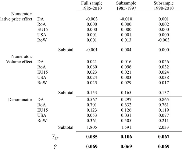
Table 7 reports the elements needed for the evaluation of the BoP-constrained growth rate

following Equation (6). Broadly speaking, Vietnam’s actual growth rate was below the constrained

one during the entire period considered: 6.9% compared to 8.5% on average. This indicates that

Vietnam was respecting its BoP constraint. Equation (6) gives us further insights on the meaning of

this result. The estimation results showed that the coefficients of the relative price term are

statistically insignificant in all import equations as well as in the equations of exports to the US and

the RoW. As a consequence, the relative price effect in the numerator of Equation (6) is very small,

and income changes dominate the BoP constraint. The export volume effect (namely, the second

term in the numerator) contributes to the BoP-constrained rate by 0.153/1.805=8.5 percentage

points in aggregate, a result unaffected by the adverse but negligible relative price effect. A closer

look at Equation (6) shows that the volume effect at the numerator depends on partner countries’

growth as well as on the interaction between the bilateral income elasticities and the market shares

of exports. In particular, since the RoA has the largest export market, equal to 33.2% in the whole

sample, its contribution dominates the sum. As far as the denominator is concerned, the sum is

dominated again by the RoA, owing to its large import market shares (equal to 0.357), followed by

developing Asia, whose market share is smaller (0.194), but whose import elasticity is larger (2.9

instead of 2.0 for RoA, see Table 6). With a contribution of 0.567 and 0.701 respectively, DA and

Substantial differences emerge however when we analyse separately the two subperiods before and

after the Asian crisis. While the actual growth rate displays a surprising stability, the constraint

shifts between the first and the second subsample. Before the East Asian crisis, Vietnam grew at a

rate below the BoP-constrained one, with a spread of 4.1 percentage points. The large part of trade

that occurred with the former Soviet bloc countries may partially explain the much higher growth

rate predicted by the model for this subperiod. Still, the sustained rapid growth achieved by the

country after Doi Moi illustrates a situation where productive capacity was underutilised within the

planned economy and the transition reforms brought resources into production. Thus, Vietnam

between 1985 and 1997 may be described as capacity constrained, with the country growing at its

capacity growth rate without encountering BoP difficulties.

The reverse occurs in the second subperiod, where Vietnam’s actual growth rate marginally

exceeded the BoP-constrained one (6.9% compared to 6.7%), resulting in capital inflows to bridge

the financing gap. The spread between the BoP equilibrium and the actual averages, which

decreased from 4.1 to about -0.2 percentage point, can be taken as evidence of an increased demand

constraint on Vietnam’s growth. As a matter of fact, the constrained growth rate fell from 10.6% to

6.7% after the Asian crisis, while the country actually kept growing at 6.9%. As a consequence, the

question arises as to why was Vietnam’s BoP-equilibrium growth rate falling? Which partners were

responsible for this and through which channel of transmission?

(Insert Figure 2 here)

Table 7 allows us to answer these questions by separately reporting the terms of the summations at

the numerator and the denominator of Eq. (6). We should remark at the outset that since the

estimated elasticities are constant and the relative price effects are negligible over the whole

sample, any change between the first and the second subsample must come from either the

evolution of the market shares, or a change in a partner’s growth rate, or both. At an aggregate

level, we observe that the evolution of the constraint was determined by both a decrease in the

15

the former was smaller (in percentage terms) than the latter (the numerator decreased by 18.6% and

the denominator increased by 27.7%). As for the numerator, the strongest effect which contributed

to tightening Vietnam’s BoP came from the volume of exports destined to the RoA. With the

heaviest weight in the bilateral income elasticity of exports, the RoA (namely, the developed Asia)

sustained Vietnam’s export growth over the whole period considered (Figure 2). However, its GDP

growth rate declined by 2 percentage points in the second subperiod, eroding Vietnam’s export

performance. A Bilateral Trade Agreement (BTA) signed in 2000 between Vietnam and the US

evidently boosted Vietnamese exports. But this only partially compensated the former negative

effect In fact, the US contribution in the first subsample was negligible, therefore, although it

increased tenfold (from 0.3 percentage point to 3.8), its contribution was unable to offset the fall of

the RoA export volume effect to one third (from 9.6 to 3.2).

As for the denominator of Equation (6), its increase from 1.59 to 2.03 between the two subperiods

is explained mainly by the evolution of the trade relations with the other Asian countries. While

Vietnam was mainly dependent on imports from the Rest of Asia over the whole period considered,

the most relevant change came from the share of the Developing Asia in Vietnam’s total imports.

Since this market share climbed from 10.1% before the Asian crisis to 29.6% in the last subperiod,

the corresponding weighted bilateral elasticity rose sharply from 0.31 to 0.9. This indicates a strong

asymmetry in bilateral trade relations between Vietnam and its developing neighbours: the country

exports mainly to the advanced countries (with the highest export sensitivity to income changes for

the US), but any rise in domestic activity will imply a sustained growth of imports from the

Developing Asia.

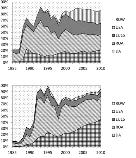
Figure 2 depicts the evolution of Vietnam’s trade market shares over the period considered: as

bilateral flows grew at different rates, the market shares evolved accordingly. Even if the bilateral

income elasticities remained constant, the denominator changed over time and impacted negatively

(2005), whose estimates for import behaviour demonstrated that Vietnam’s growth is highly

dependent on imported capital and intermediate goods. After the regional crisis in 1997, its appetite

for imports coming from Asia reached 1.62 out of 2.03 in the denominator. Thus, the greater the

rate of capacity utilisation through exports, the greater the extent of necessary imports to keep

production moving.

V. Impact of the current global crisis

A last step of our study assesses the impact of the current global crisis on Vietnam’s economic

growth. More precisely, the over reliance on the high income markets for exports has been

questioned since 2008. In order to address this issue, we look at the evolution over time of the BoP

constrained rate. Since the BoP constraint is in its nature a long-run constraint, we evaluate it using

the long-run components of the relevant variables, and compare it with an estimate of the long-run

growth rate.

The long-run component of each series was extracted using the Hodrick and Prescott (1997) filter.

The filter computes the smoothed (long run) component st of a series yt by minimising the variance

of the deviation of yt from st, subject to a penalty that constrains the second differences of the

smoothed series. The long-run component st thus minimizes the following expression:





_





 







The  parameter equals 100, namely the value suggested by Hodrick and Prescott (1997) when

dealing with annual data.

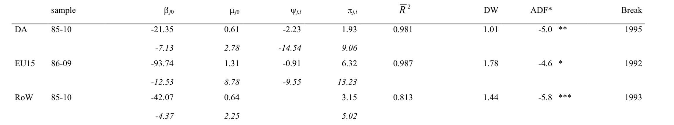
(Insert Figure 3 here)

The filtered series were then inputted in Equation (6), providing us with a time varying estimate of

the BoP constraint. The estimate allows us to confirm the previous results (Figure 3). After

17

constrained growth before 1993, the country grew almost at the same rate as the one predicted by

the model until 2005, started to violate its BoP constraint. This outcome was not caused by an

acceleration in growth, as the historical rates remained almost stable, but because of a tightening of

the BoP constraint since 2005, determined by the evolution of the bilateral market shares and

partners’ growth rates. Export growth made a significant contribution to GDP growth, but the shift

to a more import intensive pattern of growth contributed to deteriorating the BoP position of

Vietnam, whose export growth was affected by economic slowdown in the RoA, while the import

growth was simultaneously accelerated by the process of regional integration (notably towards

Developing Asia).

Growth targets and the global economic turmoil

Vietnam’s Socio Economic Development Strategy (SEDS) for the period 2011 to 2020 identifies

the country’s key priorities over the current decade. The overall goal is for Vietnam to lay the

foundations for a modern, industrialised society by 2020. Accordingly, the government aspires to

achieve by that year a per capita income level of 3000 current USD. This translates into a nearly

10% annual growth in per capita nominal GDP over the decade (World Bank, 2011). To meet this

ambitious target, the Vietnamese National Assembly set a target for real GDP growth of around

6.5-7% annually under the five year Socio Economic Development Plan 2011-2015 (SEDP), . The

total export receipts are expected to increase by 13%. Gross capital accumulation would occupy

33.5–35% of GDP in this period, while the trade deficit rate would be gradually reduced from 2012

onwards and is expected to be 10% of total export turnover by 2015.

The question addressed here is whether the government’s medium-run growth target is achievable

in the context of a weaker global economic environment, and how the foreign exchange

requirements will be filled to meet this target. To this purpose, we depart from the last assessment

of GDP growth edited by the International Monetary Fund (IMF, 2012). We constructed our

with the filtered series for import and export market shares.7 _{The corresponding BoP equilibrium}

growth rate is calculated by substituting our estimates of the long-run income and price elasticities.

(Insert Table 8 here)

According to IMF projections, growth prospects differ across the partner areas: while the

Developing Asia is expected to maintain a high growth rate (7.8% per year on average), activity in

the Northern partners (the RoA, the EU and the US) will remain rather low. The relatively high

growth rate in the RoW is attributable to the recent dynamic expansion of South–South trade,

providing developing countries with a favourable external economic climate for export expansion

(Bagnai et al., 2012). Vietnam is expected by the IMF to keep growing at a rate of 6.7% per year,

which is consistent with the government’s target (Table 7).

Our baseline scenario shows that, provided that all the partner areas confirm the growth rates

projected by the IMF for the period from 2011 to 2017, Vietnam’s BoP constraint would be relaxed

in comparison with the 1998-2010 subperiod, because of high demand growth in the RoA, the US

and the RoW. The growth rate predicted by the model lifts up (8.2%), enabling the country to

achieve its growth target without encountering BoP problems.

However, in case the current crisis in the euro area does not lead to visible improvement in the

external environment, this relevant change could be reversed. In this perspective, three scenarios are

compared here. Scenario 1 assumes a sharp recession in the world economy, with a decrease in all

partners’ GDP growth by one percentage point with respect to the baseline. Under scenario 2, the

same slowdown in GDP growth affects only the Northern partners (the RoA, the US and the EU).

Finally, scenario 3 hypothesizes that the Asian area is able to avoid the economic turmoil.

Under scenario 1, recession in all partner areas, with the associated slowdown in the demand for

Vietnam’s exports, will tighten the BoP constraint to 5.2%. As a result, the government growth

target could be achieved only through a heavier reliance on capital inflows. Under scenario 2, when

19

only the Northern partners are affected by the economic turmoil, Vietnam’s BoP constraint is less

binding; but the corresponding growth rate (5.5%) remains lower than the government’s target and

far lower than the growth rate estimated in the baseline. In other words, a demand led expansion in

South–South trade may be a weak alternative engine of export expansion. Whatever the scenario

undertaken, the ongoing recession reveals the vulnerability of Vietnam’s growth to the external

economic climate, as the production networks built in the Asian area work to its disadvantage. To

illustrate this argument, scenario 3 results in more optimistic projections by assuming that the

Asian area is sheltered from the global crisis. In this case Vietnam’s BoP–constrained growth rate is

close to the target (6.2% against 6.5%), allowing the government to achieve the medium-run growth

rate without further increases in capital inflows to bridge the financing gap. In other words,

continued robust economic expansion in the Asian region would attenuate the negative impact on

Vietnam of what would otherwise be a global economic downturn.

VI. Conclusion

Vietnam has made important progress in achieving economic and social development over the past

two decades. The country’s accession to the WTO paved the way to greater market liberalisation

and foreign investment inflows. However, recent developments in Vietnam’s economic conditions

suggest that the country’s BoP problems come from its integration into global and regional

economies. In the face of rapid growth with structural change in trade partnerships, the connection

between BoP and growth cannot be ignored.

In view of this, our paper examines the long-run relationship between economic growth and the

current account balance equilibrium using a multi-country BoP constrained growth model. This

model allows us to assess whether the country growth was compatible with its BoP equilibrium, and

what are the international factors that could prevent any attempt to achieve a sustained growth of

and we analysed separately the two subsamples before and after the 1997 Asian crisis, looking at

the possible role of the different trading partners in the evolution of the BoP constraint.

Our results show that over the whole sample Vietnam respected its BoP constraint. However, our

decomposition allows us to identify the international mechanisms through which Vietnam’s BoP

position worsened, related to the nature of the country’s trade partnership before and after the Asian

crisis. While before the crisis (1985-1997) the Vietnamese economy was well inside its BoP

constraint, after the crisis the constraint tightened quickly. The estimation results show that this

outcome does not depend on the evolution of relative prices, whose effect is neutral. The evolution

of the BoP constraint is dominated by changes in the market shares and in the partners’ growth rate.

In particular, Vietnam has partially benefited from a change in bilateral or multilateral trade policies

with advanced countries (for instance, through the US-VN bilateral trade agreement). However,

Vietnamese growth is hindered by the ‘appetite’ for imports coming from the whole of Asia. This

feature is consistent with a production oriented trade structure which has proliferated in the region,

often as a part of triangular (South–South–North) trading networks. Finally, the study addressed the

issue of the impact of global recession on Vietnam’s growth for the period 2011 to 2017. The

scenario analyses show that slower growth in the partner areas will result in a BoP constraint well

below the government medium-run growth target. However, the capital inflows needed to fill the

foreign exchange gap are relatively limited in case the Asian partners keep growing and remain

unaffected by the global economic turmoil.

Since exports represent a source of foreign exchange, the analysis developed here provides a

rationale for an export-led growth strategy. However, our results suggest that this strategy is highly

vulnerable to the external economic environment, notably through the constraint imposed by the

21

References

Abbott, P., Bentzen, J. and Tarp, F. (2009) Trade and development: Lessons from Vietnam’s past

trade agreements, World Development, 37, 341-353.

Bagnai, A., Rieber, A. and Tran, T.A.D. (2012) Generalised BoP constrained growth and

South-South trade in Sub Saharan Africa, in Models of Balance of Payments Constrained Growth:

History, Theory and Empirical Evidence (Eds) E. Soukiazis and P.A. Cerqueira, Palgrave

MacMillan, Basingstoke, 113-143.

Campbell, J.Y. and Perron, P. (1991) Pitfalls and opportunities: what macroeconomists should

know about unit roots, in NBER Macroeconomics Annuals 1991, Vol. 6, MIT Press, Cambridge

MA, 141-201.

Dickey, D. and Fuller, W. (1979) Distribution of the estimators for autoregressive time series with a

unit root, Journal of the American Statistical Association, 74, 427-431.

Dolado, J., Jenkinson, T. and Sosvilla-Rivero, S. (1990) Cointegration and unit roots, Journal of

Economic Surveys, 4, 249–73.

Elder, J. and Kennedy, P.E. (2001) Testing for unit roots: what should students be taught?, Journal

of Economic Education, 32, 137-46.

Engle, R.F. and Granger, C.W.J. (1987) Cointegration and error correction: representation,

estimation and testing, Econometrica, 55, 251-276.

Felipe, J., McCombie, J.S.L. and Naqvi, K. (2009) Is Pakistan’s growth rate Balance of Payments

constrained? Policies and implications for development and growth, Asian Development

Economics, Working Paper Series, No.160, Asian Development Bank, Manila.

Gregory, A.W. and Hansen, B.E. (1996) Residual based tests for cointegration in models with

regime shifts, Journal of Econometrics, 70, 99-126.

Hodrick, R.J. and Prescott, E.C. (1997) Postwar U.S. Business Cycles: An Empirical Investigation,

Hussain, M.N. (1999) The Balance of Payment Constraint and Growth Rate Differences among

African and East Asian Economies, African Development Review, 11, 103-137.

IMF (2012) World Economic Outlook, International Monetary Fund, Washington D.C., October.

Nell, K.S. (2003) A ‘generalised’ version of the Balance-of-Payments growth model: an application

to neighbouring regions, International Review of Applied Economics, 17, 249-267.

Otero, J. and Smith, J. (2000) Testing for cointegration: power versus frequency of observation –

further Monte Carlo results, Economic Letters, 67, 5-9.

Sapsford, D. and Chen, J.R. (1998) The Prebisch-Singer Terms of Trade Hypothesis: Some (Very)

New Evidence, in Development Economics and Policy (Eds) D. Sapsford and J.R. Chen,

Macmillan, London.

Sepheri, A. and Akram-Lodhi, A.H. (2005) Transition, Savings and Growth in Vietnam: A Three

gap Analysis, Journal of International Development, 17, 553-574.

Soukiazis, E. and Antunes, M. (2011-12) Application of the Balance-of-Payments constrained

growth model to Portugal, 1965-2008, Journal of Post-Keynesian Economics, 34, 353-379.

Thirlwall, A.P. (1979) The Balance of Payments Constraint as an Explanation of International

Growth Rate Differences, Banca Nazionale del Lavoro Quarterly Review, 128, 45-53.

Thirlwall, A.P. (2012) Balance of Payments Constrained Growth Models: History and Overview, in

Models of Balance of Payments Constrained Growth: History, Theory and Empirical Evidence

(Eds) E. Soukiazis and P.A. Cerqueira, Palgrave MacMillan, Basingstoke, 11-49.

World Bank (2008) Vietnam Development Report 2009: Capital Matters, Vietnam Consultative

Group Meeting, Hanoi, December.

World Bank (2011) Vietnam Development Report 2012: Market Economy for a Middle income

23

Appendix A. Countries

Group A (Developing Asia, DA): Bangladesh, Bhutan, Cambodia, China, India, Indonesia, Lao

PDR, Malaysia, Mongolia, Nepal, Pakistan, Philippines, Sri Lanka, Thailand.

Group B (Rest Of Asia, RoA): Australia, Brunei, French Polynesia, Hong Kong, Japan, Macao,

New Caledonia, New Zealand, North. Mariana Islands, Singapore, South Korea.

Group C (EU15): Austria, Belgium, Denmark, Finland, France, Germany, Greece, Ireland, Italy,

Luxembourg, Netherlands, Portugal, Spain, Sweden, United Kingdom.

Group D: USA

Group E: Rest of the World (RoW)

Appendix B. Data sources and definitions

The bilateral trade flows of Vietnam to and from each partner region were reconstructed using the

Comtrade database. The sample runs from 1985 through 2010. Missing data in the bilateral trade

series were reconstructed as follows: if either of the two flows is missing, we use its ‘mirror’. If

instead they are both reported but with different values, the bilateral series are reconstructed as a

weighted average of the import and the export ones (where imports receive a 2/3 weight). The data

on the bilateral trade relations between Vietnam and the RoW are missing from the beginning of the

sample through 1997. The two series were reconstructed taking for each the difference between the

total flow, extracted from the World Development Indicators (WDI) database, and the sum of the

other bilateral flows. Then we calculated the RoW flows by subtracting from the total the other four

bilateral trade series.

Since the Comtrade series are in USD at current prices, in order to get their real counterparts, the

import series Mj were deflated using country j aggregate export deflator (evaluated as the ratio of

nominal to real exports in USD), while the export series Xj were deflated using Vietnam export

deflator (evaluated accordingly). Vietnam export deflator was missing from 1985 to 1988. The

aggregate exports and GDP come from the 2012 edition of the WDI database. All real variables are

measured in USD at 2000 prices.

Relative prices were constructed as the ratio of domestic prices (measured by Vietnam export

deflator) to foreign prices (measured by partner j GDP deflator). The estimation was also performed

using a terms of trade variable constructed as the ratio of Vietnam export deflator to the partner

export deflator (that is, to Vietnam import deflator). The empirical results (available upon request)

did not compare favourably with the one presented in the paper.

Appendix C. Unit root tests

As is well known, the results of unit root tests are strongly dependent on the correct specification of

the deterministic component (drift and trend) of the underlying Data Generating Process (DGP).

Misspecification of the deterministic component may entail a loss of power (see Campbell and

Perron, 1991). In order to cope with this issue, we adopted the testing strategy proposed by Elder

and Kennedy (2001). In short, this strategy uses the a priori information, provided by the pattern of

the time series, in order to rule out those alternative hypotheses that are inconsistent with the

observed behaviour of the data. This allows the researcher to decide on both the correct

specification of the deterministic component and the presence of a unit root using a single test, thus

reducing the multiple hypotheses testing issues presented by other testing strategies (such as the one

proposed by Dolado et al., 1990).

First, the plot of the series is inspected, in order to verify whether it exhibits a trending behaviour. If

the series is trending, we perform an F test for the null hypothesis H0: =1, =0 in the model:

yt =  + t +  yt-1 + t

This F statistic has a non standard distribution under the null and is compared with the critical

values of the 3 statistic provided by Dickey and Fuller (1979). Failure to reject the null implies

25

(namely, <1, 0). The other possible alternatives are ruled out, being inconsistent with the

observed data behaviour (see Elder and Kennedy, 2001).

If instead the series does not display a regular trending behaviour, we test the null hypothesis

H0:=1, =0 in the model:

yt =  +  yt-1 + t

In this case the F statistics follows the 1 distribution by Dickey and Fuller (1979). Failure to reject

implies that the series is I(1) without drift, while rejection implies that the series was generated by

an I(0) process with unconditional mean different from zero. In both cases, lags of the differenced

dependent variable were added to the equation in order to whiten its residuals. The lag length was

determined by reduction, starting from a maximum order of lags equal to 2, which was deemed

appropriate considering the sample length and the fact that we are using annual data.

The results of the tests are summarized in Table A1. All the variables, except relative prices, display

a clear trending behaviour, that could be compatible with either a I(1) with drift process, or with a

I(0) process with deterministic trend. The relative price series, instead, display a pronounced

reversal occurring at the beginning of the 1990s, which is incompatible with the presence of a

deterministic trend. The results show that in all cases we were unable to reject the unit root null.

Table A1. Unit root tests

variable behaviour statistic lags variable behaviour statistic lags

mA,t trending 3.17 0 xA,t trending 2.20 0

mB,t trending 2.46 1 xB,t trending 1.53 0

mC,t trending 3.63 0 xC,t trending 1.76 0

mD,t trending 2.27 0 xD,t trending 5.33 0

mE,t trending 0.77 0 xE,t trending 5.60 1

yA,t trending 2.20 1 rA,t non trending 2.31 0

yB,t trending 3.84 0 rB,t non trending 2.73 0

yC,t trending 3.25 1 rC,t non trending 2.75 0

yD,t trending 4.59 2 rD,t non trending 2.17 0

yE,t trending 2.79 0 rE,t non trending 2.15 0

yt trending 5.77 1

For trending series we applied the 3 test and for non trending series the 1 test by Dickey and Fuller (1981). The 5%

Figures and tables

Figure 1. Vietnam’s external balance

Sources: Trade balance, UN Comtrade and General Statistics Office of Vietnam (GSO); Current account balance, IMF

World Economic Outlook.

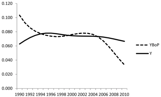
Figure 2. Export and import market shares (respectively in volume and in value)

-35 -30 -25 -20 -15 -10 -5 0 5 10 1985 1987 1989 1991 1993 1995 1997 1999 2001 2003 2005 2007 2009 Trade Balance Current Account Balance

Trade Balance GSO

0% 10% 20% 30% 40% 50% 60% 70% 80% 90% 100% 1985 1990 1995 2000 2005 2010 ROW USA EU15 ROA DA 0% 10% 20% 30% 40% 50% 60% 70% 80% 90% 100% 1985 1990 1995 2000 2005 2010 ROW USA EU15 ROA DA

Export market shares

27

Figure 3. The HP series of BoP equilibrium and actual growth rates

Table 1. Bilateral imports equations, Engle and Granger estimation

sample _{j i,j i,j DW CRADF}

DA 1985-2010 -29.54 -0.42 3.63 0.96 0.69 -1.81 -15.48 -1.94 19.49 RoA 1985-2010 -18.53 -0.39 2.63 0.94 0.622 -2.28 -11.60 -2.62 16.98 EU15 1985-2010 -12.28 -0.12 1.87 0.93 1.119 -3.05 -9.80 -1.01 15.22 EU15 1985-2010 -12.97 1.94 0.93 1.049 -2.94 -12.28 18.69 USA 1994-2010 -18.14 0.52 2.35 0.87 1.763 -3.44 -7.66 1.12 10.41 USA 1994-2010 -18.22 2.36 0.87 1.653 -3.24 * -7.64 10.39 RoW 1985-2010 -4.16 0.61 0.73 0.42 1.268 -3.48 -8.25 -1.76 12.09

The t-statistics are reported in italic under the coefficient estimates. DW is the statistic of the Durbin-Watson test, CRADF is the cointegrating residual augmented Dickey-Fuller test. An asterisk indicates rejection at the 10% level.

0.000 0.020 0.040 0.060 0.080 0.100 0.120 1990 1992 1994 1996 1998 2000 2002 2004 2006 2008 2010 YBoP Y 2 R

Table 2. Bilateral imports equations, Gregory and Hansen estimation

j0 j0 i,j i,j DW ADF* Break

DA -23.99 1.15 -0.17 3.00 0.985 1.99 -7.49 *** 1991 -16.20 6.19 -1.24 19.51 DA -24.44 1.22 3.03 0.984 1.84 -6.63 *** 1991 -16.84 6.75 19.93 RoA -12.77 1.27 -0.02 1.97 0.984 1.76 -5.55 *** 1991 -11.82 8.13 -0.26 17.25 RoA -12.76 1.29 1.96 0.985 1.78 -5.54 *** 1991 -12.08 9.81 17.71 EU15 -7.89 0.64 -0.10 1.40 0.959 2.29 -5.72 *** 1993 -5.28 3.91 -1.12 9.03 EU15 -8.20 0.73 1.42 0.97 2.25 -5.60 *** 1992 -7.28 5.46 12.04 RoW 16.44 -16.99 0.25 -1.38 0.68 3.00 -4.53 1991 3.58 -2.88 1.60 -2.95 RoW -5.27 -0.99 0.92 0.44 1.82 -4.57 * 1990 -2.77 -3.96 4.63

j0 is the intercept, j0 the shift in the intercept, i,j the relative prices elasticity, i,j the income elasticity. The t-statistics are reported in italic under the coefficient estimates. DW

is the statistic of the Durbin-Watson test, ADF* is the statistic of the Gregory and Hansen test for the null of non cointegration. One (two, three) asterisk indicates a 10% (5%, 1%) significant statistic.

2

29

Table 3. Bilateral exports equations, Engle and Granger estimation

sample j  j,i j,i DW CRADF

DA 1985-2010 -28.0 -2.2 2.4 0.98 0.645 -3.15 -13.6 -12.6 17.2 RoA 1985-2010 -112.2 -0.8 7.7 0.98 0.998 -5.58 *** -20.8 -7.2 22.3 EU15 1985-2010 -138.5 -1.0 9.2 0.95 0.335 -2.34 -13.1 -5.0 13.8 USA 1994-2010 -178.7 -0.6 11.5 0.95 1.124 -3.75 * -15.7 -1.0 16.4 USA 1994-2010 -180.2 11.6 0.95 1.153 -3.85 ** -16.0 16.7 RoW 1985-2010 -50.6 -0.3 3.7 0.80 1.322 -3.81 * -6.3 -1.7 7.2 RoW 1985-2010 -58.2 4.2 0.78 1.314 -3.63 * -8.4 9.5

The t-statistics are reported in italic under the coefficient estimates. DW is the statistic of the Durbin-Watson test, CRADF is the cointegrating residual augmented Dickey-Fuller test. An asterisk indicates rejection at the 10% level.

2

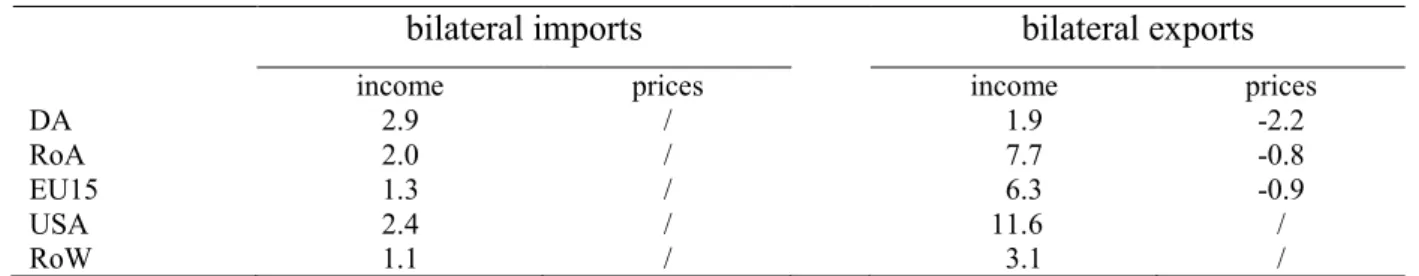
Table 4. Bilateral exports functions, Gregory and Hansen estimation

sample j0 j0 j,i j,i DW ADF* Break

DA 85-10 -21.35 0.61 -2.23 1.93 0.981 1.01 -5.0 ** 1995 -7.13 2.78 -14.54 9.06 EU15 86-09 -93.74 1.31 -0.91 6.32 0.987 1.78 -4.6 * 1992 -12.53 8.78 -9.55 13.23 RoW 85-10 -42.07 0.64 3.15 0.813 1.44 -5.8 *** 1993 -4.37 2.25 5.02

j0 is the intercept, j0 the shift in the intercept, j,i, the relative prices elasticity, j,i, the income elasticity. The t-statistics are reported in italic under the coefficient estimates. DW

is the statistic of the Durbin-Watson test, ADF* is the statistic of the Gregory and Hansen test for the null of non cointegration against the alternative of a level shift. One (two, three) asterisk indicates a 10% (5%, 1%) significant statistic.

2

31

Table 5. Bilateral imports functions, FMOLS estimation

sample j,i DW DA 1985-2010 2.92 2.11 25.12 RoA 1985-2010 1.96 1.95 21.46 EU15 1985-2010 1.34 2.28 13.07 USA 1994-2010 2.41 1.63 9.68 RoW 1985-2010 1.07 1.91 5.76

The t-statistics are reported in italic under the coefficient estimates. DW is the statistic of the Durbin-Watson test.

Table 6. A summary of the estimated elasticities

bilateral imports bilateral exports

income prices income prices

DA 2.9 / 1.9 -2.2

RoA 2.0 / 7.7 -0.8

EU15 1.3 / 6.3 -0.9

USA 2.4 / 11.6 /

Table 7. Comparison between the BoP equilibrium and the actual growth rates Full sample 1985-2010 Subsample 1985-1997 Subsample 1998-2010 Numerator:

Relative price effect DA -0.003 -0.010 0.001

RoA 0.000 0.000 0.002 EU15 0.000 0.000 0.000 USA 0.001 0.001 0.000 RoW 0.001 0.013 -0.003 Subtotal -0.001 0.004 0.000 Numerator: Volume effect DA 0.021 0.016 0.026 RoA 0.060 0.096 0.032 EU15 0.023 0.021 0.024 USA 0.024 0.003 0.038 RoW 0.025 0.029 0.017 Subtotal 0.153 0.165 0.137 Denominator DA 0.567 0.297 0.865 RoA 0.701 0.632 0.761 EU15 0.123 0.126 0.119 USA 0.053 0.031 0.077 RoW 0.361 0.505 0.211 Subtotal 1.805 1.591 2.033 0.085 0.106 0.067 0.069 0.069 0.069

Table 8. Some projections on Vietnam’s economic growth (2011-2017)

Baseline:

IMF projections Scenario 1 Scenario 2 Scenario 3

Partner’s growth DA 0.078 0.068 0.078 0.078 RoA 0.021 0.011 0.011 0.021 EU15 0.016 0.006 0.006 0.006 USA 0.028 0.018 0.018 0.018 RoW 0.040 0.030 0.040 0.030 0.082 0.052 0.055 0.062 0.065 0.065 0.065 0.065 BP Y Y BP Y et t Y arg