Meta-analysis of multidecadal biodiversity trends
in Europe
Francesca Pilotto
et al.
#Local biodiversity trends over time are likely to be decoupled from global trends, as local
processes may compensate or counteract global change. We analyze 161 long-term biological
time series (15–91 years) collected across Europe, using a comprehensive dataset comprising
~6,200 marine, freshwater and terrestrial taxa. We test whether (i) local long-term
biodi-versity trends are consistent among biogeoregions, realms and taxonomic groups, and (ii)
changes in biodiversity correlate with regional climate and local conditions. Our results reveal
that local trends of abundance, richness and diversity differ among biogeoregions, realms and
taxonomic groups, demonstrating that biodiversity changes at local scale are often complex
and cannot be easily generalized. However, we
find increases in richness and abundance with
increasing temperature and naturalness as well as a clear spatial pattern in changes in
community composition (i.e. temporal taxonomic turnover) in most biogeoregions of
Northern and Eastern Europe.
https://doi.org/10.1038/s41467-020-17171-y
OPEN
#A list of authors and their affiliations appears at the end of the paper.
123456789
T
he current biodiversity crisis, manifested in a global decline
of species, affects many taxonomic groups and biotic
realms
1–4. These changes may be less evident at specific
locations, since local factors, such as small-scale colonization and
species turnover may compensate or even counteract trends
occurring at larger spatial scales. Heterogeneity in patterns of
change in biodiversity observed at a local scale
5,6has been
described in several studies. For example, strong declines in local
biomass and distribution have been reported for terrestrial
insects
7–10and birds
11–13, but reports of local increases in
bio-diversity are also widespread and span multiple taxonomic
groups
5including freshwater invertebrates
14,15,
fishes
16, birds
12,13and plants
17–19.
Ecosystem functions and their benefits to people at local to
global scales ultimately depend on the taxonomic and functional
diversity of local communities
5,20. The same relationship applies
to conservation measures: while they need to be harmonized at
larger scales, most measures need to be tailored to local
condi-tions. Therefore, it is crucial to understand the variation in
bio-diversity trends between localities and how and why these may
vary across biota, regions and local conditions
21.
Analyses of the trends in local biodiversity over large spatial
scales and multiple taxonomic groups are needed to fully
understand the patterns of local biodiversity change and the
discrepancies between local and global biodiversity trends.
Unfortunately such syntheses are rare. Current evidence from
multi-taxa biodiversity trend comparisons is limited and
equi-vocal, and direct comparison across studies is hampered by
substantial differences in the temporal and spatial coverage and
resolution of the data. Dornelas et al.
6studied 100 time series of
terrestrial, freshwater and marine taxonomic groups around the
world and found no systematic temporal changes in
α-diversity of
local communities. However, the authors detected significant
increases in
β-diversity and increasing trends in species richness
for terrestrial plants in the temperate region
6. The most
com-prehensive study to date to our knowledge
22showed that species
turnover, i.e., a measure of temporal community variability, is
stronger in marine than freshwater and terrestrial assemblages
and that this is often decoupled from changes in species richness.
However, these results were based on a relatively coarse spatial
and temporal resolution, and mostly short time series. Other
studies focused on a smaller number of sites or more restricted
biotic scope. A study of 22 sites in different realms from Central
Europe detected stronger effects of temperature on population
trends in terrestrial than aquatic habitats (i.e. populations of
terrestrial
“species with warmer temperature preferences
increased more than [terrestrial] species with colder temperature
preferences” (page 3), but found no such relationship for aquatic
taxa)
23. Finally, Gibson-Reinemer et al.
24found that the
increasing species turnover in mountain communities was
stronger in ectotherm communities and in tropical compared to
temperate regions. These results point towards region, biotic, and
realm specific patterns in local biodiversity trends, but a
prehensive overview directly comparing trends among
com-plementary time series has been lacking so far.
The present study analyzes trends in various taxonomic groups
measured at specific locations in nine different biogeoregions
across the European continent. We ask: (1) are long-term trends
in biodiversity detectable at individual localities across Europe?
(2) If so, to what extent are such trends attributable to changes in
climate at a regional scale and/or changes in local conditions? (3)
Do observed trends in biodiversity vary predictably among
bio-georegions, realms and taxonomic groups and, thus, inform our
understanding and prediction of larger scale patterns? Due to the
ongoing global change we expect to observe: (1) long-term
reductions in biodiversity indicated by declining species richness
and abundances (2) increasing variability in community
com-position, indicated by higher temporal species turnover and (3)
differential responses across taxonomic groups and
biogeor-egions, reflecting differences in the extent of and vulnerability to
climate change (i.e. Southern Europe should be more negatively
affected than Northern Europe
25).
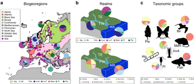
We compile 161 long-term (minimum 15 years) biomonitoring
time series from 115 sites, mostly belonging to the International
Long-Term Ecological Research network (ILTER
26), in 21 European
countries (Fig.
1
), covering nine biogeoregions, three realms and
eight taxonomic groups (Fig.
1
, Supplementary Table 1,
Supple-mentary Data). For each time series, we compute total abundance of
the community, taxonomic richness, diversity and temporal
turn-over and estimated their monotonic trends turn-over the study period.
Biogeoregions
b
a
Realmsc
TE TE FW FW MA MA Taxonomic groups Alpine Atlantic Black Sea Boreal Continental Mediterranean Pannonian North Sea Adriatic Sea Outside SiteAlpine Atlantic Black Sea Boreal
Continental Mediterranean North Sea Pannonian
Alg Alg Bir Bir Fish Fish InvA InvA
InvT Mam InvT
Mam Pl
Pl Pla
Pla
Alg Bir Fish InvA InvT Mam Pl Pla
Adriatic Alpine Atlantic Black Sea Boreal
Continental Mediterranean North Sea Pannonian
Adriatic
Fig. 1 Distribution of the time series across biogeoregions, realms and taxonomic groups. a Relative distribution of studied taxonomic groups across biogeoregions (magenta dots: study sites). Note that the most south-eastern site (in Israel) belongs to the Mediterranean region.b Relative distribution of studied taxonomic groups and biogeoregions across realms.c Relative distribution of studied biogeoregions across taxonomic groups. FW freshwater, MA marine and transitional zone, TE terrestrial, Alg benthic algae, Bir birds, InvA aquatic invertebrates, InvT terrestrial invertebrates, Mam mammals, Pl plankton, Pla terrestrial plants. The pie charts show the proportion of taxonomic groups for each biogeoregion and realm, and the proportion of biogeoregions for each realm and taxonomic group. The shapefiles of the biogeographical regions and marine subregions were obtained from EEA74.
We then apply a meta-analytic approach to identify the patterns
among biogeoregions, realms and taxonomic groups. Our time
series have an unbalanced distribution across biogeoregions, realms
and taxonomic groups, which is a common issue in macroecological
studies
6,22,23. We account for the unbalanced design by testing the
robustness of our results using a sensitivity analysis (Supplementary
notes) and when interpreting the results. Our results show that
trends in common biodiversity metrics differ among biogeoregions,
realms, and taxonomic groups. Particularly, we
find stronger
changes in community composition in Northern and Eastern
Europe and increases in richness and abundance with increasing
temperature and naturalness.
Results
Overall trends. We observed overall increasing trends in
taxo-nomic richness, diversity and turnover, across all time series,
while there was no significant trend in abundance (Table
1
).
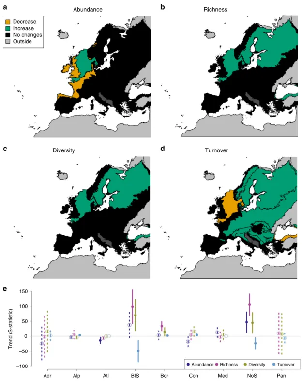
Biodiversity trends. The trends of all biodiversity metrics
dif-fered among biogeoregions (Table
1
). Abundances declined in the
Atlantic region and increased in the North Sea over time. Species
richness and diversity increased in the Black Sea, Boreal region
and North Sea. Species turnover increased over time in time series
from the Alpine, Boreal and Continental regions, and decreased
in time series from the Black Sea and North Sea (Table
1
, Fig.
2
).
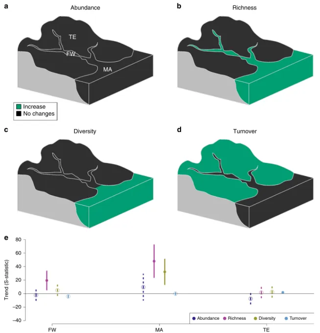
We did not detect any clear trends in abundance in any realm,
while trends in taxon richness, diversity and turnover varied
across realms. We recorded increasing taxon richness in the
freshwater realm, increasing taxon richness and diversity in the
marine realm, and increasing turnover in the terrestrial realm
(Table
1
; Fig.
3
).
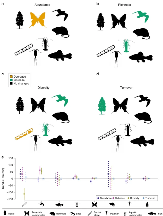
We found a significant decline in the abundance of terrestrial
invertebrates. Species richness, diversity and turnover trends
differed among taxonomic groups (Table
1
). Species richness and
diversity increased in birds and aquatic invertebrates. This
contrasted with the decreasing diversity in benthic algae (note
that algae data were only available for sites within a single river
catchment). Turnover trends significantly increased for plants.
Other taxa did not show a trend in the respective biodiversity
metrics (Table
1
, Fig.
4
).
Influence of climatic trends and site characteristics. The most
important predictors (i.e., highest absolute values of z-scores) of
abundance and richness trends were site naturalness (i.e., a
measure of local anthropogenic pressure), temperature trend (i.e.,
S-statistics of air or water temperature trend, according to the
realm) and their interaction (Table
2
). Increases in temperature
and site naturalness were correlated with increased abundance
and richness. The negative interaction between site naturalness
and temperature trend indicates stronger increases in abundance
and richness with increasing temperature at sites with lower
naturalness than at sites with high naturalness (Supplementary
Fig. 1). The most important predictor of diversity trends was
longitude (positive correlation). Species turnover trends were
mostly affected by elevation (positive correlation) and by the
positive interaction between site naturalness and temperature
trend, indicating stronger increases in turnover with increasing
temperature at sites with higher naturalness than at sites with low
naturalness (Table
2
, Supplementary Fig. 1). Study length had
much less influence on the trends, indicating that the differences
in study intervals among time series did not bias our results
(Table
2
).
Discussion
Our results demonstrate considerable heterogeneity in the extent
and direction of change in biodiversity metrics in recent decades
between biogeoregions, realms and taxonomic groups in Europe.
We identified increases in taxon richness in Northern and Eastern
Europe. Records in these regions are primarily represented by
terrestrial and aquatic invertebrate datasets. These observed
pat-terns are in line with recent modelled predictions of future
responses to global changes
25and are likely due to
climate-change induced poleward range shifts across taxa
27–30. We also
detected declines in species abundances for terrestrial
inverte-brates and in the Atlantic biogeoregion (from which most of the
Table 1 Biodiversity trends.
Abundance Richness Diversity Turnover
Overall trend z −1.4 2.95 2 3.59 d.f. 152 160 160 160 p 0.162 0.003 0.045 0.003 Biogeoregion Wald-type test of model coefficients QM 24.397 65.83 21.23 38.6 d.f. 8 9 9 9 p 0.002 <0.001 0.012 <0.001 Atlantic z −2.73 p 0.006 North Sea z 2.73 5.77 2.55 −2.42 p 0.006 <0.001 0.011 0.015 Black Sea z 3.41 2.67 −2.73 p <0.001 0.008 0.006 Boreal z 4.35 2.09 2.05 p <0.001 0.037 0.04 Alpine z 3.79 p <0.001 Continental z 2.49 p 0.01 Realm Wald-type test of model coefficients QM 4.17 22.75 12.58 13.15 d.f. 3 3 3 3 p 0.243 <0.001 0.006 0.004 Freshwater z 2.73 p 0.006 Marine z 3.9 3.37 p <0.001 <0.001 Terrestrial z 3.25 p 0.001 Taxonomic group Wald-type test of model coefficients QM 24.67 57.09 20.06 d.f. 8 8 8 p 0.002 <0.001 0.01 Terrestrial invertebrates z −2.95 p 0.003 Birds z 4.11 4.78 p <0.001 <0.001 Aquatic invertebrates z 2.42 2.26 p 0.015 0.024 Benthic algae z −5.33 p <0.001 Plants z 3.7 p <0.001
Biodiversity trends for the whole dataset (overall trends) and within the different biogeoregions, realms and taxonomic groups, as resulting from meta-analysis mixed models. Note that only
significant results (p ≤ 0.05) are reported for the biogeoregion, realm and taxonomic
terrestrial invertebrate time series in our dataset are derived). Our
results, based on data with larger spatial, temporal and taxonomic
coverage, and
finer temporal resolution, corroborate recent
reports of worldwide declines of local terrestrial insect
commu-nities
31–33.
Several studied biogeoregions, realms and biotic groups
showed no significant trends in biodiversity metrics. Other
studies on local changes in biodiversity also detected no overall
changes
5,22,34in apparent contradiction to the documented
global-scale biodiversity loss (e.g. IPBES
4). However, the
extinc-tion of rare species, by definiextinc-tion, is often restricted to the very
few local places where these species occur and may thus go
undetected in large extent quantitative studies
35. Furthermore,
the loss of specialist taxa could be compensated locally by the
Abundance Richness Diversity
e
Turnover Decrease Increase No changes Outside 150 100 Trend (S-statistic) 50 0 –50 –100Adr Alp Atl BIS Bor Con
Abundance Richness Diversity Turnover
Med NoS Pan
a
c
d
b
Fig. 2 Biodiversity trends in the different biogeoregions. The results of meta-analysis mixed models are shown for the four studied biodiversity metrics: abundance (a), richness (b), diversity (c) and turnover (d). Green: significant increasing trends (p ≤ 0.05); orange: significantly declining trends (p ≤ 0.05); black (dark grey for Adriatic Sea): no significant trends (p > 0.05). For biogeoregion identity see Fig.1.e Values of S-statistics (model estimated mean, error bar:+/− C.I.). Adr: Adriatic (n = 1 time series), Alp: Alpine (n = 33 time series), Atl Atlantic (n = 56 time series), BlS Black Sea (n = 5 time series), Bor Boreal (n= 32 time series), Con Continental (n = 17 time series), Med Mediterranean (n = 9 time series), NoS North Sea (n = 7 time series), and Pan Pannonian (n= 1 time series). Dark blue: abundance, pink: richness, yellow: diversity, light blue: turnover. Solid line and dot: p ≤ 0.05; dashed line and open circle: p > 0.05. Source data are provided as a Source Datafile.
colonization of more tolerant and generalist species
36and/or
invasive taxa, resulting in biotic homogenization despite no
change in overall species richness
36,37. Such patterns were, for
example, observed in vascular plants at coarse scales in Europe
due to the extinction of rare native species and spread of alien
species
38. Thus, temporal changes in taxonomic composition, i.e.,
turnover, are likely to be more sensitive than simply taxonomic
richness (i.e., alpha-diversity) and abundance in responses to
global change
39,40. Accordingly, we show that temporal changes
in taxon turnover are more pertinent across biogeoregions than
the other three studied biodiversity metrics. The observed
increases in temporal taxon turnover are spatially structured
across Europe, involving mostly biogeoregions of Northern and
Eastern Europe. Such changes in community composition can
reflect non-equilibrium dynamics (including time-lags and
tran-sient phenomena
41) with, for example, climate change
42,
pollution or the introduction and spread of alien species
43.
Moreover, over the past 30–40 years (i.e. the period covered by
most time series in our dataset) positive impacts of environmental
regulation, e.g., reductions in atmospheric emissions and hence
acid rain, could also be important drivers of biotic change (see
e.g., Monteith et al.
44). In a recent analysis of UK vegetation data,
an overall increase in vegetation species richness was linked to
recovery from acidification
45. Accordingly, increases in species
turnover could also reflect a process of biological recovery from
past disturbances. Another possible interacting factor is the
change in land use, which follows different temporal trajectories
in different European regions, and thus could concur in
explaining regional differences in biodiversity trends
46. Future
research should clarify to what extent the increasing taxon
turnover is led by the spread of generalist and invasive species
compared to declines in rare species, and whether the observed
MA TE FW Abundance Richness Diversity Increase No changes TurnoverAbundance Richness Diversity Turnover 80 60 40 20 0 –20 –40 FW MA TE Trend (S-statistic)
a
b
c
d
e
Fig. 3 Biodiversity trends in the three realms. The results of meta-analysis mixed models are shown for the four studied biodiversity metrics: abundance (a), richness (b), diversity (c) and turnover (d). Green: significant increasing trends (p ≤ 0.05); black: no significant trends (p > 0.05). e Values of S-statistics (model estimated mean, error bar:+/−C.I.). Dark blue: abundance, pink: richness, yellow: diversity, light blue: turnover. Solid line and dot: p ≤ 0.05; dashed line and open circle: p > 0.05. FW freshwater (n= 51 time series); MA marine and transitional zones (n = 18 time series); TE terrestrial (n = 92 time series). Source data are provided as a Source Datafile.
changes are due to direct human impact, indirect effects (see e.g.,
Didham et al.
47, in the context of biological invasions) or recovery
processes
48.
Our model results showing positive correlations of temperature
and naturalness with richness and abundance trends are
consistent with other studies, e.g.
14,25. However, we could also
identify a combined effect of naturalness and temperature on
abundance, richness and turnover trends. More specifically, and
counterintuitive to common expectation, we found that sites
considered to be in a less natural state are those experiencing the
Abundance Richness Diversity Turnover Decrease Increase No changes
e
a
c
d
b
150 100 Trend (S-statistic) 50 0 –50 –100–150 Abundance Richness Diversity Turnover
Plants Terrestrial
invertebrates Mammals Birds
Benthic
algae Plankton
Aquatic
invertebrates Fish
Fig. 4 Biodiversity trends for the studied taxonomic groups. The results of meta-analysis mixed models are shown for the four studied biodiversity metrics: abundance (a), richness (b), diversity (c) and turnover (d). Green: significant increasing trends (p ≤ 0.05); orange: significant declining trends (p≤ 0.05); black: no significant trends (p > 0.05). Drawings from phylopic.org. e values of S-statistics (model estimated mean, error bar: +/−C.I.). Dark blue: abundance, pink: richness, yellow: diversity, light blue: turnover. Solid line and dot: p≤ 0.05; dashed line and open circle: p > 0.05. Number of time series (n): Plants: 34, terrestrial invertebrates: 53, mammals: 1, birds: 16, benthic algae: 7, plankton: 9, aquatic invertebrates: 38,fish: 3. Source data are provided as a Source Datafile.
strongest changes in biodiversity metrics with increasing
tem-perature (i.e. steeper increase in abundance and richness and
steep decline in turnover). We speculate that degraded sites are
more prone to invasion of generalist and invasive species, while
natural sites may be more resilient
49.
A major obstacle in assessing biodiversity trends is that
long-term data are unevenly distributed among taxonomic groups and
are biased towards charismatic taxa, such as birds and mammals,
and towards groups with long study traditions, such as vascular
plants and marine
fishes, while invertebrates are relatively
neglected, except butterflies and bees in some countries. Our
study encompasses an unusually large variety of taxonomic
groups, including those largely overlooked in previous large-scale
biodiversity studies
6,20. Some of these overlooked groups that we
included in our analysis, such as aquatic invertebrates, showed
unexpected increases in richness and diversity, likely due to the
aforementioned processes (e.g. recovery from stressors, spread of
generalist or invasive taxa and taxa adapted to warmer
tem-peratures). On the other hand, we recorded declines in species
abundances for terrestrial invertebrates in the Atlantic
biogeor-egion, consistent with previous
findings
31,32,50. Our results
therefore emphasize that patterns of change in the biodiversity of
the most studied
‘iconic’ groups cannot be extrapolated across
other taxa.
These
findings reiterate the need to not only maintain but to
increase the numbers of long-term monitoring schemes of local
ecosystems. Such schemes can provide unique insights for
ecol-ogists and conservationists, yet they are often threatened by a lack
of support as they do not
fit into the temporal extent of most
funding schemes. In contrast to space-for-time or aggregated
snapshot (e.g. opportunistic data or atlases of species
distribu-tions) approaches, the long-term tracking of communities in
specific locations minimizes the risk of biases related to shifts in
sampling locations, sampling areas and protocols
51.
Our dataset is, to the best of our knowledge, the most
com-prehensive in terms of the spatial and temporal extent and
taxonomic and realm representation of high temporal resolution
long-term biodiversity monitoring records in Europe. Most sites
included in this study are part of the global ILTER network and
the vast majority are characterized by low anthropogenic
pres-sure, which may have led to an underestimation of the true scale
of biodiversity changes at continental scale. Perhaps most
importantly, most studied sites are shielded from direct effects of
changes in land-use and loss of habitat, e.g., conversion to
intensive agriculture and urbanization. To overcome such sources
of bias, long-term monitoring programs should include a larger
representation of more intensively used (e.g. agricultural) areas
and incorporate sites vulnerable to significant anthropogenic
perturbations
51. On the other hand, our approach reduces the
potential risk of tracking immediate biodiversity responses to
localized disturbance or successional recovery processes, which
can bias the estimates of biodiversity change
52.
Although most of our time series do not predate the 1980s
(only one study goes back to the 1920s), we were still able to
detect evidence of substantial reorganization of communities
within relatively short time frames. However, our data, as well as
most of the data used in other studies
6,10,22,23, is being considered
in the absence of the longer historical perspective required to
capture the overall changes in biodiversity in the Anthropocene,
as we lack baseline data from times when human impacts were
lower (e.g. pre-industrial era). This limitation is a common issue
in studies of long-term biodiversity change (but see ref.
53) that
can have a detrimental effect in restoration ecology
54,55. The lack
of baseline data could be overcome by the integration of
ecolo-gical and paleobioloecolo-gical approaches (e.g. Battarbee et al.
56),
which could extend the temporal dimension back to, e.g., the end
of the last ice age. Such approaches could have important
con-servation implications
57and allow for comparisons between
impacted and unimpacted sites within the same geographical
area, which could reveal differences between changes driven by
climate and by direct anthropogenic pressures (e.g. changes in
land use or pollution)
58. Looking into the future, there is an
urgent need to harmonize biodiversity monitoring schemes
59,60that would also allow improved up- and downscaling of trends as
well as integrating cross-domain feedback loops
61.
The inherent complexity of ecological systems manifested by
diverging long-term responses of local biodiversity still hamper
any upscaling of these trends to a continental or even global scale.
This might explain the partly contradictory results not only
within but also among large-scale studies that are based on local
biodiversity data
6,22. For example, our study revealed higher
taxon turnover in the terrestrial realm at European scale while, at
a global scale, turnover seems higher in marine assemblages
22.
However, these studies do agree on the lack of an overall decline
in species richness and on the increase in taxon turnover over
time. We argue that these contradictory results can be driven by
the insufficient number and quality of systemic and harmonized
biodiversity monitoring activities at a local scale and by the
insufficient length of the underlying time series. Regarding the
latter, we should bear in mind that prior to the start of most of
our biodiversity time series (mainly in the 1980s), many species
had already declined in abundance or gone extinct. Moreover, the
vast majority of larger scale studies describing biodiversity
changes have not been able to clearly identify the environmental
Table 2 In
fluence of climatic trends and site characteristics
on biodiversity trends.
Explanatory variables z Abundance Intercept −1.48 Temperature trend 1.22 Precipitation trend 0.18 Naturalness 1.73 Latitude −0.99 Study length −0.30Temperature trend: Naturalness −2.39
Richness Intercept 3.66 Temperature trend 2.04 Precipitation trend 0.38 Naturalness 1.14 Latitude 0.49 Longitude 2.16 Elevation −1.20 Study length 0.37
Temperature trend: Naturalness −2.02
Diversity Intercept 1.97 Temperature trend −0.56 Precipitation trend −2.05 Latitude −0.49 Longitude 3.49 Elevation −1.66 Study length 1.27 Turnover Intercept 3.35 Temperature trend −0.60 Precipitation trend 1.66 Naturalness −0.52 Latitude 1.66 Longitude −1.21 Elevation 4.09 Study length 1.03
Temperature trend: Naturalness 3.39
drivers of these changes. This demonstrates the urgent need to
complement biodiversity time series with environmental data that
can be used to explain the observed patterns but are often not
collected on a routine basis (with exceptions in limnology and
oceanography). The complexity of biodiversity dynamics that our
results and those of other studies highlight is not to be interpreted
as an obstacle to the development of conservation measures.
Rather we argue that a better understanding of the patterns,
trends and changes in biodiversity and environmental conditions
will allow conservation measures to be better tailored to specific
locations and taxonomic groups in order to significantly retard or
even reverse further biodiversity loss
62.
Methods
Data compilation. We circulated a call for biodiversity data within the ILTER network and additional partners tofill in geographical gaps. The criteria for data selection were: (1) each time series covers at least 15 years, (2) with preferably at least ten survey events during that time, (3) sampling occurred at the same site (no space-for-time substitution), and (4) survey method, seasonal and taxonomic resolution were consistent throughout the whole study period for each time series. Thefinal dataset included 161 time series from 89 ILTER sites and 26 additional long-term monitoring sites from other networks. The time span of the studied time series ranged between 15 and 91 years (median: 20), so that one time series started in 1921 while the others started between the 1980 and 2003 (median: 1994). The end years range between 2005 and 2018 (median: 2015; Supplementary Fig. 2). Biodiversity data. Biodiversity data were expressed as abundance or biomass of surveyed taxa at each survey occasion, in some instances as percent coverage (e.g. for some time series of benthic algae and plants). Survey methods and season varied among time series, but were kept constant within each time series throughout the entire study period. In most cases, surveys were carried out once a year, but some time series had gaps or more frequent survey intervals (e.g. weekly resolution for phytoplankton, zooplankton and moths from the Finnish and Czech sites). In the latter case, wefiltered the data in the time series to select only the months/seasons that were consistently surveyed throughout the whole study per-iod, and we pooled the data (as sums or averages) within each year. Taxonomic resolution was kept constant for each time series throughout the entire study period, generally at the species or genus level, with a few exceptions (i.e. a few macroinvertebrates groups were identified at family resolution).
For each year within each time series, we computed four biodiversity metrics: total number of organisms or biomass (hereby referred to as abundance), taxonomic richness (i.e. number of taxa), Simpson´s diversity and temporal taxon turnover. The latter was computed as the proportion of taxa gained and lost between two subsequent years relative to the total number of taxa observed, using Eq. (1), as implemented in the R package codyn63.
Number of taxa gained þ number of taxa lost
total number of taxa : ð1Þ
We classified the time series into nine biogeoregions, three realms and eight taxonomic groups (Fig.1).
Abiotic variables. For each study site we extracted the daily mean temperature and daily total precipitation data from the gridded observational dataset for pre-cipitation, temperature and sea level pressure in Europe (spatial resolution: 0.25 degrees64), and computed the mean annual temperature and total annual pre-cipitation. For aquatic ecosystems we used in situ water temperature measured at the surface and calculated the mean temperature across the yearly monitoring periods.
We gathered information on local anthropogenic pressures in a standardized questionnaire (Supplementary Methods). The questionnaire asked the data providers to assess the impact (from 1= no to 4 = strong impact) of a series of pressures at the site (e.g. urbanization, sources of pollution, agriculture, etc.; for a full list see Supplementary Methods) and indicate whether impacts were constant or changed throughout the study period. Data providers were also asked to estimate the overall environmental quality of the site (i.e. naturalness; from 1= low to 5= high) and to state whether it was constant or changed throughout the study period. We used this information to define the quality-class of the sites, based on the overall assessment. The majority of sites (n= 67) scored 5 (i.e. high naturalness), 42 sites scored 4, 37 sites scored 3 and 15 sites scored 2. Data analysis. We used a two-step procedure that allowed us to combine very heterogeneous original datasets (see paragraph Biodiversity data). First, we ana-lyzed each time series separately to quantify time-series-specific biodiversity trends. Second, we used the effect sizes of the individual time-series-specific biodiversity trends to synthesize the overall trends and identify common patterns and drivers. The results of this second (meta-)analysis are reported in the paper.
For thefirst step of the analysis, we used the Mann–Kendall trend test to identify monotonic trends in each biodiversity and climate time series over the study period65,66. We detected serially correlated time series using auto- and cross-covariance and correlation functions67, and we applied the modified
Mann–Kendall with Hamed and Rao68variance correction approach. We used S-statistic and its variance as effect size of the trend65for the next step of the analysis. A similar meta-analytical approach has already been applied in a previous study on ecological time series69.
At 23 study sites, multiple time series were available for a given taxonomic group, e.g., when surveys were conducted at multiple transects or plots or with multiple traps. To avoid pseudoreplication, we combined those time series using meta-analysis mixed models (using the R package metafor70) and extracted the cumulative effect sizes and their variances prior to the second step of the analysis. The total of 161 time series reported above refers to the aggregatedfinal set of time series.
The second step of the analysis aimed at synthesizing the trends across the different time series. For that, wefitted meta-analysis mixed models to account for random effects. To compute the overall biodiversity trends and to explore how the trends varied among biogeoregions, realms and taxonomic groups, we included biogeoregion (nine levels), realm (three levels: freshwater, marine and transitional zone, and terrestrial) and taxonomic group (eight levels) as explanatory variables in the models with no intercept. We did so separately because biogeoregion, realm and taxonomic group were not independent (see Supplementary Table 1). The results of these models hence show whether or not the overall S-statistics for individual trends in the groups differ significantly from zero.
Additional meta-analysis mixed models were used to test the influence of selected abiotic variables describing site characteristics and climate on the biodiversity trends. We included the following variables: latitude, longitude, elevation, site naturalness, S-statistics65of temperature and precipitation trends, and the length of each time series. These explanatory variables showed little collinearity (|r| < 0.6), and were thus all retained as potential predictors. Similar to Everaert et al.71, we applied an information-theoretic approach to model selection and multi-model inference72, to determine the relative importance of those explanatory variables on the trends in biodiversity metrics. For this we created a candidate set of models with all possible linear combinations of explanatory variables and we extracted the corrected Akaike's information criterion (AICc) of each model using the R package glmulti73. We retained only plausible models with δAICc ≤ 2 of the best model (i.e. the one(s) with the lowest AICc72) and computed the relative importance of each predictor variable as the sum of the Akaike's weights of all the selected models in which that variable was included. We computed the model-averaged coefficients (±95% C.I.) for each predictor variable in each selected model, weighted by the Akaike's weights (Supplementary Table 2). To evaluate the effect of the interaction among climatic and local stressors, we added to the selected models the interactions between site naturalness and temperature trends, and the interaction between site naturalness and precipitation trends. We then compared the resulting models (without interaction, with single interaction, with both interactions) and chose the one with the lowest AIC value. We have implemented this procedure because, to the best of our knowledge, it is not possible to include selected interactions into the information-theoretic approach to model selection and including all interactions would have resulted in an overly complex model.
To account for biases in biogeoregions, realms and taxonomic groups, we also performed sensitivity analyses (Supplementary notes and Supplementary Table 3), which confirmed that the results were robust.
Reporting summary. Further information on research design is available in the Nature Research Reporting Summary linked to this article.
Data availability
All datasets analyzed during the current study have been deposited in public repositories, at the links reported in Supplementary Data. Please note that some of the datasets will be publicly accessible after a period of embargo, from 1st January 2021. The source data underlying allfigures are provided as a Source Data file. Source data are provided with this paper.
Code availability
The R code used for all analyses is available at the GitHub repository:https://github.com/ Biodiversity-trends-in-Europe-ILTER/R-code. Source data are provided with this paper.
Received: 20 November 2019; Accepted: 16 June 2020;
References
1. WWF. Living Planet Report 2016. Risk and Resilience in a New Era. (Gland, Switzerland: WWW International, 2016).
2. Johnson, C. N. et al. Biodiversity losses and conservation responses in the Anthropocene. Science 356, 270–275 (2017).
3. Dirzo, R. et al. Defaunation in the Anthropocene. Science 345, 401–406 (2014). 4. IPBES. Summary for policymakers of the global assessment report on
biodiversity and ecosystem services of the Intergovernmental Science-Policy Platform on Biodiversity and Ecosystem Services. (IPBES secretariat, 2019). 5. Sax, D. F. & Gaines, S. D. Species diversity: from global decreases to local
increases. Trends Ecol. Evol. 18, 561–566 (2003).
6. Dornelas, M. et al. Assemblage time series reveal biodiversity change but not systematic loss. Science 344, 296–299 (2014).
7. Conrad, K. F., Warren, M. S., Fox, R., Parsons, M. S. & Woiwod, I. P. Rapid declines of common, widespread British moths provide evidence of an insect biodiversity crisis. Biol. Conserv. 132, 279–291 (2006).
8. Goulson, D., Lye, G. C. & Darvill, B. Decline and conservation of bumble bees. Annu. Rev. Entomol. 53, 191–208 (2008).
9. Thomas, J. A. Butterfly communities under threat. Science 353, 216–218 (2016).
10. Hallmann, C. A. et al. More than 75 percent decline over 27 years in total flying insect biomass in protected areas. PLoS ONE 12, e0185809 (2017). 11. Chamberlain, D. E. & Fuller, R. J. Local extinctions and changes in species
richness of lowland farmland birds in England and Wales in relation to recent changes in agricultural land-use. Agric. Ecosyst. Environ. 78, 1–17 (2000). 12. Inger, R. et al. Common European birds are declining rapidly while less
abundant species’ numbers are rising. Ecol. Lett. 18, 28–36 (2015). 13. Rosenberg, K. V. et al. Decline of the North American avifauna. Science 366,
120–124 (2019).
14. Haase, P. et al. Moderate warming over the past 25 years has already reorganized stream invertebrate communities. Sci. Total Environ. 658, 1531–1538 (2019).
15. Baranov, V., Jourdan, J., Pilotto, F., Wagner, R. & Haase, P. Complex and nonlinear climate-driven changes in freshwater insect communities over 42 years. Conserv. Biol.https://doi.org/10.1111/cobi.13477(2020).
16. Martinho, F. et al. Does theflatfish community of the Mondego estuary (Portugal) reflect environmental changes? J. Appl. Ichthyol. 26, 843–852 (2010).
17. Knapp, S., Kühn, I., Stolle, J. & Klotz, S. Changes in the functional composition of a Central European urbanflora over three centuries. Perspect. Plant Ecol. Evol. Syst. 12, 235–244 (2010).
18. Förster, A., Becker, T., Gerlach, A., Meesenburg, H. & Leuschner, C. Long-term change in understorey plant communities of conventionally managed temperate deciduous forests: effects of nitrogen deposition and forest management. J. Veg. Sci. 28, 747–761 (2017).
19. Steinbauer, M. J. et al. Accelerated increase in plant species richness on mountain summits is linked to warming. Nature 556, 231–234 (2018). 20. Vellend, M. et al. Global meta-analysis reveals no net change in local-scale
plant biodiversity over time. Proc. Natl Acad. Sci. USA 110, 19456–19459 (2013).
21. Primack, R. B. et al. Biodiversity gains? The debate on changes in local- vs global-scale species richness. Biol. Conserv. 219, A1–A3 (2018).
22. Blowes, S. A. et al. The geography of biodiversity change in marine and terrestrial assemblages. Science 366, 339–345 (2019).
23. Bowler, D. E. et al. Cross-realm assessment of climate change impacts on species’ abundance trends. Nat. Ecol. Evol. 1, s41559–016 (2017). 0067–016. 24. Gibson-Reinemer, D. K., Sheldon, K. S. & Rahel, F. J. Climate change creates
rapid species turnover in montane communities. Ecol. Evol. 5, 2340–2347 (2015).
25. Domisch, S. et al. Modelling distribution in European stream
macroinvertebrates under future climates. Glob. Change Biol. 19, 752–762 (2013).
26. Mirtl, M. et al. Genesis, goals and achievements of Long-Term Ecological Research at the global scale: a critical review of ILTER and future directions. Sci. Total Environ. 626, 1439–1462 (2018).
27. Parmesan, C. et al. Poleward shifts in geographical ranges of butterfly species associated with regional warming. Nature 399, 579–583 (1999).
28. Walther, G.-R. et al. Ecological responses to recent climate change. Nature 416, 389–395 (2002).
29. Parmesan, C. & Yohe, G. A globally coherentfingerprint of climate change impacts across natural systems. Nature 421, 37–42 (2003).
30. Pöyry, J., Luoto, M., Heikkinen, R. K., Kuussaari, M. & Saarinen, K. Species traits explain recent range shifts of Finnish butterflies. Glob. Change Biol. 15, 732–743 (2009).
31. Seibold, S. et al. Arthropod decline in grasslands and forests is associated with landscape-level drivers. Nature 574, 671–674 (2019).
32. Sánchez-Bayo, F. & Wyckhuys, K. A. G. Worldwide decline of the entomofauna: a review of its drivers. Biol. Conserv. 232, 8–27 (2019). 33. Simmons, B. I. et al. Worldwide insect declines: an important message, but
interpret with caution. Ecol. Evol. 9, 3678–3680 (2019).
34. Valtonen, A. et al. Long‐term species loss and homogenization of moth communities in Central Europe. J. Anim. Ecol. 86, 730–738 (2017). 35. Thomas, C. D. Local diversity stays about the same, regional diversity
increases, and global diversity declines. Proc. Natl Acad. Sci. USA 110, 19187–19188 (2013).
36. Larsen, S., Chase, J. M., Durance, I. & Ormerod, S. J. Lifting the veil: richness measurements fail to detect systematic biodiversity change over three decades. Ecology 99, 1316–1326 (2018).
37. Olden, J. D. & Poff, N. L. Toward a mechanistic understanding and prediction of biotic homogenization. Am. Nat. 162, 442–460 (2003).
38. Winter, M. et al. Plant extinctions and introductions lead to phylogenetic and taxonomic homogenization of the Europeanflora. Proc. Natl Acad. Sci. USA 106, 21721–21725 (2009).
39. Hillebrand, H. et al. Biodiversity change is uncoupled from species richness trends: Consequences for conservation and monitoring. J. Appl. Ecol. 55, 169–184 (2018).
40. Antão, L. H., Pöyry, J., Leinonen, R. & Roslin, T. Contrasting latitudinal patterns in diversity and stability in a high-latitude species-rich moth community. Glob. Ecol. Biogeogr. 29, 896–907 (2020).
41. Hastings, A. et al. Transient phenomena in ecology. Science 361, eaat6412 (2018).
42. Gaüzère, P., Iversen, L. L., Barnagaud, J.-Y., Svenning, J.-C. & Blonder, B. Empirical predictability of community responses to climate change. Front. Ecol. Evol. 6, 186 (2018).
43. Essl, F. et al. Socioeconomic legacy yields an invasion debt. Proc. Natl Acad. Sci. USA 108, 203–207 (2011).
44. Monteith, D. T. et al. Biological responses to the chemical recovery of acidified fresh waters in the UK. Environ. Pollut. 137, 83–101 (2005).
45. Rose, R. et al. Evidence for increases in vegetation species richness across UK Environmental Change Network sites linked to changes in air pollution and weather patterns. Ecol. Indic. 68, 52–62 (2016).
46. Kuemmerle, T. et al. Hotspots of land use change in Europe. Environ. Res. Lett. 11, 064020 (2016).
47. Didham, R. K., Tylianakis, J. M., Hutchison, M. A., Ewers, R. M. & Gemmell, N. J. Are invasive species the drivers of ecological change? Trends Ecol. Evol. 20, 470–474 (2005).
48. Martínez‐Abraín, A., Jiménez, J. & Oro, D. Pax Romana: ‘refuge
abandonment’ and spread of fearless behavior in a reconciling world. Anim. Conserv. 22, 3–13 (2019).
49. Kröel-Dulay, G. et al. Increased sensitivity to climate change in disturbed ecosystems. Nat. Commun. 6, 1–7 (2015).
50. Simmons, B. I. et al. Worldwide insect declines: an important message, but interpret with caution. Ecol. Evol. 9, 3678–3680 (2019).
51. Cardinale, B. J., Gonzalez, A., Allington, G. R. H. & Loreau, M. Is local biodiversity declining or not? A summary of the debate over analysis of species richness time trends. Biol. Conserv. 219, 175–183 (2018).
52. Gonzalez, A. et al. Estimating local biodiversity change: a critique of papers claiming no net loss of local diversity. Ecology 97, 1949–1960 (2016). 53. Habel, J. C. et al. Butterfly community shifts over two centuries. Conserv. Biol.
30, 754–762 (2016).
54. Soga, M. & Gaston, K. J. Shifting baseline syndrome: causes, consequences, and implications. Front. Ecol. Environ. 16, 222–230 (2018).
55. Silliman, B. R. et al. Are the ghosts of nature’s past haunting ecology today? Curr. Biol. 28, R532–R537 (2018).
56. Battarbee, R. W. et al. Recovery of UK lakes from acidification: An assessment using combined palaeoecological and contemporary diatom assemblage data. Ecol. Indic. 37, 365–380 (2014).
57. Barnosky, A. D. et al. Merging paleobiology with conservation biology to guide the future of terrestrial ecosystems. Science 355, eaah4787 (2017). 58. Albrecht, J. et al. Logging and forest edges reduce redundancy in
plant-frugivore networks in an old-growth European forest. J. Ecol. 101, 990–999 (2013).
59. Kareiva, P., Marvier, M. & Silliman, B. Effective Conservation Science: Data Not Dogma. (Oxford University Press, 2017).
60. Haase, P. et al. The next generation of site-based long-term ecological monitoring: Linking essential biodiversity variables and ecosystem integrity. Sci. Total Environ. 613–614, 1376–1384 (2018).
61. Heffernan, J. B. et al. Macrosystems ecology: understanding ecological patterns and processes at continental scales. Front. Ecol. Environ. 12, 5–14 (2014). 62. Harvey, J. A. et al. International scientists formulate a roadmap for insect
conservation and recovery. Nat. Ecol. Evol. 4, 174–176 (2020).
63. Hallett, L. et al. codyn: Community Dynamics Metrics. R package version 2.0.0. (2018).
64. Haylock, M. R. et al. A European daily high-resolution gridded data set of surface temperature and precipitation for 1950–2006. J. Geophys. Res. Atmospheres 113, (2008).
66. Mann, H. B. Nonparametric Tests Against Trend. Econometrica 13, 245–259 (1945).
67. Venerables, W. N. & Ripley, B. D. Modern applied statistics with S. (new york: Springer, 2002).
68. Hamed, K. H. & Rao, A. R. A modified Mann-Kendall trend test for autocorrelated data. J. Hydrol. 204, 182–196 (1998).
69. Daufresne, M., Lengfellner, K. & Sommer, U. Global warming benefits the small in aquatic ecosystems. Proc. Natl Acad. Sci. USA 106, 12788–12793 (2009).
70. Viechtbauer, W. Conducting meta-analyses in R with the metafor package. J. Stat. Softw. 36, 1–48 (2010).
71. Everaert, G., Deschutter, Y., De Troch, M., Janssen, C. R. & De
Schamphelaere, K. Multimodel inference to quantify the relative importance of abiotic factors in the population dynamics of marine zooplankton. J. Mar. Syst. 181, 91–98 (2018).
72. Anderson, D. R. & Burnham, K. P. Avoiding pitfalls when using information-theoretic methods. J. Wildl. Manag. 66, 912–918 (2002).
73. Calcagno, V. glmulti: Model selection and multimodel inference made easy. R package version 1.0.7. (2013).
74. EEA. Biogeographical regions and Marine regions and subregions under the Marine Strategy Framework Directive. https://www.eea.europa.eu/data-and-maps(2016).
Acknowledgements
We are grateful to the ILTER network and the eLTER PLUS project (Grand Agreement No. 871128) forfinancial support. We acknowledge the E-OBS dataset from the EU-FP6 project ENSEMBLES (http://ensembles-eu.metoffice.com) and the data providers in the ECA&D project (http://www.ecad.eu). The evaluation of forest plant diversity was based on data collected by partners of the official UNECE ICP Forests Network (http://icp-forests.net/contributors); part of the data were co-financed by the European Commission, project LIFE 07 ENV/D/000218“Further Development and Imple-mentation of an EU-level Forest monitoring Systeme (FutMon)”. Data on wintering water birds in Bulgaria were provided by the national Executive Environment Agency with the Ministry of Environment and Waters. Data from the Finnish moth monitoring scheme were supported by the Finnish Ministry of the Environment. Data from the Swedish ICP Integrated Monitoring sites werefinanced by the Swedish Environmental Protection Agency. Data collection at Esthwaite Water and a subset of UK ECN sites was supported by Natural Environment Research Council award number NE/ R016429/1 as part of the UK-SCaPE programme delivering National Capability. Sponsorship of other UK ECN sites contributing data was provided by Agri-Food and Biosciences Institute, Biotechnology and Biological Sciences Research Council, Department of Environment Food and Rural Affairs, Natural Resources Wales, Defense Science Technology Laboratory, Environment Agency, Forestry Commission, Forest Research, the James Hutton Institute (The Rural & Environment Science & Analytical Services Division of the Scottish Government), Natural England, Rothamsted Research, Scottish Government, Scottish Natural Heritage and the Welsh Government. Data from the Mondego estuary (Portugal) were supported by the Centre for Functional Ecology Strategic Project (UID/BIA/04004/2019) within the PT2020 Partnership Agreement and COMPETE 2020, and by FEDER through the project ReNATURE (Centro 2020, Centro-01-765-0145-FEDER-000007). We would like to thank Lim-burgse Koepel voor Natuurstudie (LiKoNa) for the data related to the National Park
Hoge Kempen (BE). We would like to acknowledge the support for the long-term monitoring program MONEOS in the Scheldt estuary (BE) by‘De Vlaamse Waterweg’ and‘Maritieme Toegang’ (Flemish government). We are grateful to the board of the National Park“De Hoge Veluwe” for the permission to conduct our research on their property. We thank Ian J. Winfield and Terje Bongard for contributing data for the sites: Bassenthwaite Lake, Derwent Water (UK) and Atna River (Norway, freshwater invertebrate time series). Open access funding provided by Umeå University.
Author contributions
F.P. and P.H. conceived the study. F.P. analyzed the data, with inputs by I.K. F.P. wrote the manuscript, with major contributions by P.H. and I.K. R. Adrian, R. Alber, A.A., C. A., J.B., L.B., D.B., N.B., S.B., D.S.B., V.B., E.C., R.C., P.C., B.J.E., G.E., V.E., H.F., R.G.G., D.G.G., U.G., J.M.G., L. Hadar, L. Halada, M.H., H.H., K.L.H., B.J., T.C.J., H.K., I.K.S., I. K., R.L., F.M., H.M., J.M., S.M., D.M., B.P.N., D. Oro, D. Ozoliņš, B.M.P., D.P., M.P., M. Â.P., B.P., T.P., J.P., S.M.S., M.S., S.C.S., A.S., K.S., G.S., R.S., J.A.S., S.S., L.S., A.T., G.V. H., G.V.R., M.E.V., S.V. and P.H. provided data and contributed to the different versions of the manuscript.
Competing interests
The authors declare no competing interests.
Additional information
Supplementary information is available for this paper at https://doi.org/10.1038/s41467-020-17171-y.
Correspondence and requests for materials should be addressed to F.P. or P.H. Peer review information Nature Communications thanks the anonymous reviewer(s) for their contribution to the peer review of this work. [Peer reviewer reports are available.]
Reprints and permission information is available athttp://www.nature.com/reprints
Publisher’s note Springer Nature remains neutral with regard to jurisdictional claims in published maps and institutional affiliations.
Open Access This article is licensed under a Creative Commons Attribution 4.0 International License, which permits use, sharing, adaptation, distribution and reproduction in any medium or format, as long as you give appropriate credit to the original author(s) and the source, provide a link to the Creative Commons license, and indicate if changes were made. The images or other third party material in this article are included in the article’s Creative Commons license, unless indicated otherwise in a credit line to the material. If material is not included in the article’s Creative Commons license and your intended use is not permitted by statutory regulation or exceeds the permitted use, you will need to obtain permission directly from the copyright holder. To view a copy of this license, visithttp://creativecommons.org/ licenses/by/4.0/.
© The Author(s) 2020
Francesca Pilotto
1,2
✉
, Ingolf Kühn
3,4,5
, Rita Adrian
6
, Renate Alber
7
, Audrey Alignier
8,9
,
Christopher Andrews
10
, Jaana Bäck
11
, Luc Barbaro
12
, Deborah Beaumont
13
, Natalie Beenaerts
14
,
Sue Benham
15
, David S. Boukal
16,17
, Vincent Bretagnolle
18,19
, Elisa Camatti
20
, Roberto Canullo
21
,
Patricia G. Cardoso
22
, Bruno J. Ens
23
, Gert Everaert
24
, Vesela Evtimova
25
, Heidrun Feuchtmayr
26
,
Ricardo García-González
27
, Daniel Gómez García
27
, Ulf Grandin
28
, Jerzy M. Gutowski
29
, Liat Hadar
30
,
Lubos Halada
31
, Melinda Halassy
32
, Herman Hummel
33
, Kaisa-Leena Huttunen
34,35
,
Bogdan Jaroszewicz
36
, Thomas C. Jensen
37
, Henrik Kalivoda
38
, Inger Kappel Schmidt
39
,
Ingrid Kröncke
40
, Reima Leinonen
41
, Filipe Martinho
42
, Henning Meesenburg
43
, Julia Meyer
40
,
Bachisio M. Padedda
48
, Denise Pallett
49
, Marco Pansera
20
, Miguel Ângelo Pardal
42
, Bruno Petriccione
50
,
Tanja Pipan
51
, Juha Pöyry
52
, Stefanie M. Schäfer
49
, Marcus Schaub
53
, Susanne C. Schneider
54
,
Agnija Skuja
47
, Karline Soetaert
33
, Gunta Spri
ņģe
47
, Radoslav Stanchev
25
, Jenni A. Stockan
55
, Stefan Stoll
56,57
,
Lisa Sundqvist
58
, Anne Thimonier
53
, Gert Van Hoey
59
, Gunther Van Ryckegem
60
, Marcel E. Visser
61
,
Samuel Vorhauser
7
& Peter Haase
1,57
✉
1Senckenberg Research Institute and Natural History Museum Frankfurt, Gelnhausen, Germany.2Environmental Archaeology Lab, Department of
Historical, Philosophical and Religious Studies, Umeå University, Umeå, Sweden.3Department of Community Ecology, Helmholtz Centre for Environmental Research - UFZ, Halle, Germany.4Martin Luther University Halle-Wittenberg, Geobotany and Botanical Garden, Halle, Germany.
5German Centre for Integrative Biodiversity Research (iDiv) Halle - Jena - Leipzig, Leipzig, Germany.6Department of Ecosystem Research, Leibniz
Institute of Freshwater Ecology and Inland Fisheries & Department of Biology, Chemistry and Pharmacy, Freie Universität Berlin, Berlin, Germany.
7Biological Laboratory, Agency for Environment and Climate Protection, Bolzano, Italy.8UMR 0980 BAGAP, INRAE– Institut Agro – ESA,
Rennes, France.9LTSER Zone Atelier Armorique, 35042 Rennes, France.10UK Centre for Ecology & Hydrology, Bush Estate, Penicuik, Midlothian, UK.11Institute for Atmospheric and Earth system Research, Department of Forest Sciences, University of Helsinki, Helsinki, Finland. 12Dynafor, INRAE, University of Toulouse, France & CESCO, Muséum National d’Histoire Naturelle, Sorbonne-Univ, Paris, France & LTSER Zone
Atelier Pyrénées Garonne, Auzeville-Tolosane, France.13Rothamsted Research, North Wyke, Okehampton, Devon, UK.14Centre for Environmental
Sciences, Hasselt University, Hasselt, Belgium.15Forest Research, Farnham, UK.16University of South Bohemia, Faculty of Science, Department of
Ecosystem Biology & Soil and Water Research Infrastructure, Ceske Budejovice, Czech Republic.17Czech Academy of Sciences, Biology Centre,
Institute of Entomology, Ceske Budejovice, Czech Republic.18CEBC, UMR7372, CNRS & La Rochelle University, 79360 Villiers en bois, France. 19LTSER Zone Atelier Plaine & Val de Sèvre, 79360 Beauvoir sur Niort, France.20Institute of Marine Sciences, National Research Council,
Venice, Italy.21School of Biosciences and Veterinary Medicine, unit Plant Diversity and Ecosystems Management, University of Camerino, Camerino, Italy.22CIIMAR, Interdisciplinary Centre of Marine and Environmental Research of the University of Porto, Porto, Portugal.23Sovon Dutch Centre for Field Ornithology, Nijmegen, The Netherlands.24Flanders Marine Institute, Ostend, Belgium.25Institute of Biodiversity and Ecosystem Research, Bulgarian Academy of Sciences, Sofia, Bulgaria.26UK Centre for Ecology & Hydrology, Lancaster Environment Centre, Lancaster, UK.27Instituto Pirenaico de Ecología (CSIC), Jaca, Spain.28Department of Aquatic Sciences and Assessment, Swedish University of Agricultural Sciences, Uppsala, Sweden.29Department of Natural Forests, Forest Research Institute, Białowieża, Poland.30Ramat Hanadiv, Zikhron Ya’akov, Israel.31Institute of Landscape Ecology SAS, Branch Nitra, Slovakia.32MTA Centre for Ecological Research, Institute of Ecology and Botany, Vácrátót, Hungary.33Royal Netherlands Institute for Sea Research, and Utrecht University, Yerseke, The Netherlands.34Department of Ecology and Genetics, University of Oulu, Oulu, Finland.35Oulanka Research Station, University of Oulu Infrastructure Platform, Kuusamo, Finland.
36Białowieża Geobotanical Station, Faculty of Biology, University of Warsaw, Białowieża, Poland.37Norwegian Institute for Nature Research,
NINA-Oslo, Norway.38Institute of Landscape Ecology SAS, Bratislava, Slovakia.39Geosciences and Natural Resource Management, University of Copenhagen, Copenhagen, Denmark.40Senckenberg am Meer, Marine Research Department, Wilhelmshaven, Germany.41Kainuu Centre for
Economic Development, Transport and the Environment, Kajaani, Finland.42Centre For Functional Ecology (CFE), Department of Life Sciences,
University of Coimbra, Coimbra, Portugal.43Northwest German Forest Research Institute, Göttingen, Germany.44Forest Services, Autonomous
Province of Bolzano - South Tyrol, Bolzano, Italy.45CEAB (CSIC), 17300 Blanes, Spain.46IMEDEA (CSIC-UIB), 07190 Esporles, Spain.47Institute of
Biology, University of Latvia, Salaspils, Latvia.48Dipartimento di Architettura, Design e Urbanistica, Università degli Studi di Sassari, Sassari, Italy. 49UK Centre for Ecology & Hydrology, Wallingford, UK.50Carabinieri, Biodiversity and Park Protection Department, Castel di Sangro Biodiversity
Unit, L’Aquila, Italy.51ZRC SAZU Karst Research Institute, Ljubljana & UNESCO Chair on Karst Education University of Nova Gorica,
Vipava, Slovenia.52Finnish Environment Institute (SYKE), Biodiversity Centre, Helsinki, Finland.53Swiss Federal Institute for Forest Snow and Landscape Research WSL, Birmensdorf, Switzerland.54Norwegian Institute for Water Research, Oslo, Norway.55Ecological Sciences, James Hutton Institute, Craigiebuckler, Aberdeen, UK.56University of Applied Sciences Trier, Environmental Campus Birkenfeld, Birkenfeld, Germany.
57University of Duisburg-Essen, Essen, Germany.58Swedish Meteorological and Hydrological Institute, Gothenburg, Sweden.59Flanders Research
Institute for Agriculture, Fishery and Food, Oostende, Belgium.60Research Institute for Nature and Forest, Brussels, Belgium.61Department of Animal Ecology, Netherlands Institute of Ecology (NIOO-KNAW), Wageningen, The Netherlands.✉email:[email protected];peter. [email protected]