3D reconstruction of the shape of optical fibers subjected to mechanical deformations

(1)

School of Industrial and Information Engineering

MSc Mechanical Engineering - Mechatronics and Robotics

3D RECONSTRUCTION OF THE SHAPE OF

OPTICAL FIBERS SUBJECTED TO

MECHANICAL DEFORMATIONS

Supervisor: Prof.ssa Paola SACCOMANDI

Co-Supervisors: Prof. Marco TARABINI, Ing. Davide PALOSCHI

Master Thesis of:

Edoardo ORIANA

Matr. Nr. 877039

(2)

(3)

(4)

(5)

Abstract

Fiber Optics, for their powerful characteristics and their capability to work in harsh environments, are widely used in diﬀerent applications (e.g., telecommunications, aerospace and mechanical engineering, biomedical applications and mechatronics) and have been studied for a long time. In particular, the interest in these materials has led to the investigation of possible applications in the sensing field.

The first chapter of this work analyzes more in detail the wide variety of fiber optics sensors. Fiber optic sensors are excellent candidates for monitoring envi-ronmental changes and oﬀer many advantages over conventional electronic sensors, thanks to their immunity to electromagnetic interference, very low mass, high sensi-tivity and high robustness. According to the classification about sensing location, operating principle and application, diﬀerent fiber optics sensors are introduced. In particular, FBGs (i.e., Fiber Bragg Gratings) written in fiber optics cores are analyzed in depth. Thanks to this technique, when a fiber optic is subjected to external perturbations (e.g., strain), the wavelength of light passing inside the core shows a particular behaviour: the input signal is filtered of a certain frequency, due to the presence of FBGs, allowing this particular wavelength of the spectrum, in phase with the grating period, to be reflected back to the input end. All other wavelengths pass through to the other end, since they are not in phase with the grating period.

The second chapter deals with the behavior of the fiber optic in the presence of external deformations. In particular, when a fiber is deformed, the wavelength reflected by the FBGs undergoes a shift of a certain value, which is proportional to the deflection.

The third and last chapter, on the other hand, deals with two diﬀerent approaches for the three-dimensional reconstruction of the fiber optic, starting from the shifts of the wavelengths. In particular, the Frenet-Serret equations and the algorithm based on homogeneous transformation matrices are compared. The main advantage of using this last approach is to reconstruct the fiber with lower computational costs and fewer interpolation points. The work then continues with the implementation of the algorithm through the Labview environment, in which the code for the real-time reconstruction of the fiber is developed.

Future work will allow for greater optimization of the code in order to further reduce the computational cost.

(6)

(7)

Acknowledgements

Prima di tutto vorrei ringraziare la mia relatrice Prof.ssa Paola Saccomandi per l’opportunità oﬀerta e per l’entusiasmante lavoro di tesi proposto, permettendomi di ampliare i miei orizzonti sulle applicazioni ingegneristiche. Ringrazio il mio correlatore Ing. Davide Paloschi per il suo grande supporto, per la sua pazienza e per i preziosissimi suggerimenti che mi ha fornito in questi mesi. Voglio ringraziare anche il Prof. Marco Tarabini per avermi suggerito questo lavoro e per avermi indirizzato verso un ottimo team.

Un ringraziamento speciale va a Beatrice, una figura fondamentale nella mia vita, che mi ha sempre prestato supporto nei momenti diﬃcili, fornendomi tutta la sicurezza e la forza necessaria per raggiungere i miei obiettivi.

Ringrazio anche i miei amici che mi hanno accompagnato in questi anni di studi. In particolare, ringrazio Sabrina, la mia amica più cara che, con quel sorriso pieno di gioia, mi ha illuminato le giornate e mi ha sempre saputo ascoltare. Cristina, che ho sempre ammirato per la sua incredibile forza d’animo nel perseguire i propri obiettivi. Marialuisa, la compagna di viaggio, che mi è sempre stata vicina e che mi ha sostenuto nel percorso di studi. Paolo, l’amico più prezioso che, oltre ad essere stato sempre presente ed avermi fornito una forte motivazione, ha saputo ampliare i miei orizzonti musicali. Ringrazio Miriam, la mia ragazza, che in questo anno buio è riuscita a farmi innamorare dopo tanto tempo.

Ringrazio infine i miei genitori, che mi hanno permesso di raggiungere questo prestigioso traguardo, supportandomi in tutte le mie scelte. Voglio ringraziare mio fratello Aurelio, che è senza dubbio il fratello migliore che qualcuno possa desiderare, sempre disponibile ad ascoltarmi e supportarmi.

(8)

(9)

Chapter 1 Introduction to Fiber Optic Sensors

This chapter analyzes the wide variety of applications for fiber optics. Used for a long time in the telecommunications field, today they are widely used for sensing and monitoring applications. Diﬀerent kinds of applications are presented, focusing on the various methods of use, technologies, and geometric parameters, introducing diﬀerent types of fiber optic sensors.

1.1 Fiber Optics Physics

The interest for signals propagation through a trasparent conduit has a fundamental importance because of the several applications in telecommunication and medical fields. As long as a transparent solid cylinder, such as a glass fiber, has a refractive index greater than that of its surrounding medium, the majority of the light which enter in one end will go out from the other end due to a large number of total internal reflections [1].

An optical fiber is constituted of a thin and flexible quartz (or glass) filament, typically with diameter of 100-200 µm, where the refractive index of the central area, called core, is generally greater than that one of the sorrounding area, called cladding. The coating or buﬀer is a layer of plastic material used to protect the optical fiber from physical damage. The buﬀer is elastic in nature and prevents abrasions [2].

Under these conditions the electromagnetic field propagate within the fiber (modes of propagation) remaining confined mainly in the core area. In terms of geometric optics, it can be said that the working principle of the optical fibers is based on the phenomenon of total reflection at the interface between the core and the cladding. Because of this phenomenon a ray of light, entering into the core with an appropriate inclination, continues to propagate and remains confined within the core itself. The main condition for this to happen, in accordance with Snell’s law of geometric optics, is that the refractive index of the core is higher than that of the cladding [1].

(11)

1.1.1 Types of Optical Fibers

From the point of view of the radial refractive index profile, optical fibers can be divided into two main categories:

(i) Graded profile, in which the refractive index of the core decreases monotonically from its maximum value, at the center of the fiber, to its minimum value at the interface between the core and the cladding. (Figure 1.1a).

(ii) Discontinuous profile, in which the refractive index of the core is radially constant and has a value higher than the one of the cladding, which is also radially constant (Figure 1.1b and 1.1c).

Figure 1.1: Diﬀerent types of optical fibers.

In terms of modes of propagation, optical fibers are classified into single-mode and multi-mode fibers; the distinction between the two cases comes from the size of the core diameter. With a suﬃciently small diameter, only one mode propagates in the optical fiber and the fiber is called single-mode. In the case of a step-index profile and for typical values of the refractive index of the core and the cladding, the value of the core diameter below which the fiber is single-mode is about 5-10 µm (depending on the wavelength). For multi-mode fibers, the typical core diameter is

instead 50-100 µm [3].

1.1.2 Considerations on Geometrical Optics

Many aspects of the behaviour of optical fibers are derived from the theory of geometrical optics.

(12)

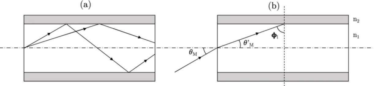
For sake of simplicity, it is considered the case of discontinuous profile fiber. Since the refractive index of the core (n1) is higher than the one of the cladding

(n2), the rays that impact the interface between the core and the cladding with a

suﬃciently large angle are subjected to the total reflection phenomenon and hence remain confined inside the core (Figure 1.2a) . For this to happen, it is necessary that the incidence angle at the interface between the core and the cladding is larger than the limit angle l (Figure 1.2b), easily obtained from Snell Law:

sin l=

n2

n1

(1.1) Therefore, the ray entering the fiber, in order to be confined inside core, has to be characterized by an incidence angle ✓ which is lower than the maximum angle ✓M,

as shown in the Figure 1.2b.

Figure 1.2: Propagation of rays inside an optical fiber with a step-index profile: (a) Internal total reflections; (b) Acceptance angle of the fiber ✓M.

The maximum angle ✓M is referred to as the acceptance angle of the fiber, and

and is defined in accordance with the Snell law and Eq.(1.1) as it follows: n0sin ✓M = n1sin ✓ 0 M = n1cos l= q n2 1 n22 (1.2)

where n0 and n1 are, respectively, the refractive indeces of core and cladding, ✓M

is the acceptance angle, and l is the limit angle. The quantity n0sin ✓M is called

Numerical Aperture (NA) of the fiber. For very small angles ✓ and for n0 ⇠= 1, the

numerical aperture is coincident with the acceptance angle [3].

1.2 Fiber Optic Sensors

The invention of the laser, dating back to 1960, has caused interest in telecommunica-tion systems through optical mediums. In particular, it has led researchers to study how to exploit the properties of optical fibers in order to use them mainly as sensors and telecommunication systems. Because of the laser capability to send a huge amount of information at a very high speed, optical fibers have become the preferred medium for transmitting light. Initially, the existence of large losses within the optical fibers, which showed signal attenuations of about 1000 dB/km, prevented the

(13)

replacement of the coaxial cables with the optical fibers, since they were not practical for communication systems. In 1969, several scientists demonstrated that the main cause of signal losses was due to impurities in the fiber material. Recent advances in fiber optics technology have significantly changed the telecommunications sector, creating fibers with low levels of impurities and thus leading to losses under 20 dB/km[11].

A further step forward in research was to combine the growth of fiber optic telecommunication products with optoelectronic devices to create fiber optic sensors. By increasing the sensitivity, it is possible to detect phase, intensity, and wavelength variations to the fiber itself, caused by external perturbations. As component prices have fallen and quality improvements have been made, the capability of fiber optic sensors to replace traditional sensors has also increased [2, 4].

Fiber optic sensors are excellent candidates for monitoring environmental changes and oﬀer many advantages over conventional electronic sensors:

– Easy to use in a wide variety of structures thanks to their small size and cylindrical geometry, including composite materials.

– Immunity to electromagnetic and radio frequency interference. – Low mass.

– Robust, more resistant to harsh environments. – High sensitivity.

– Multiplexing capability to form detection networks.

To date, fiber optic sensors have been widely used to monitor a wide range of environmental parameters such as position, vibration, deformation, temperature, humidity, viscosity, chemicals, pressure, current, electric field and many other environmental factors.

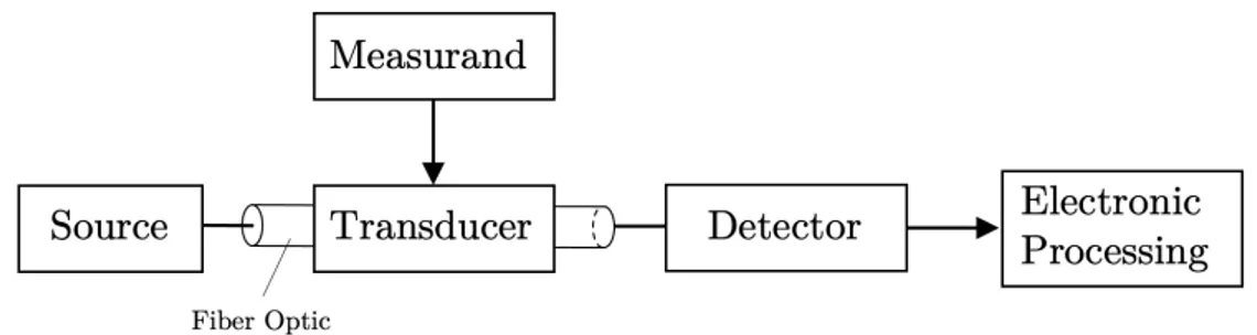
The general structure of an optical fiber sensor system is shown in Figure 1.3. It consists of an optical source (Laser, LED, Laser diode, etc.), optical fiber, sensing or modulator element (which transduces the measurand parameter to an optical signal), an optical detector and processing electronics (oscilloscope, optical spectrum analyzer, etc) [2].

(14)

Fiber optic sensors can be based on the following categories: – The sensing location.

– The operating principle. – The application.

The sensing location

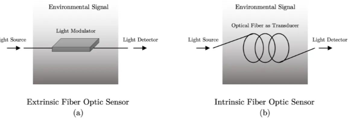
Based on the sensing location, a fiber optic sensor can be classified as extrinsic or intrinsic.

Figure 1.4: Extrinsic (a) and intrinsic (b) types of fiber optic sensors. In an extrinsic fiber optic sensor (Figure 1.4a), the fiber is simply used to transport light to an external optical device where detection occurs. In these cases, the fiber acts only as a transmission medium to bring the light into the detection position. On the other hand, in an intrinsic fiber optic sensor (Figure 1.4b), one or more physical properties of the fiber are subjected to changes and so, in turn, the characteristics of the light traveling through it [2].

The operating principle

Based on the operating principle or modulation process, a fiber optic sensor can be classified as an intensity, a phase, a frequency, or a polarization sensor. All these parameters may be subject to change due to external perturbations. Thus, the external perturbations can be sensed by detecting these parameters changes [2, 5]. The application

Based on the application, fiber optic sensors can be mainly classified as follows [2]: – Physical sensors: Used to measure physical properties like temperature, stress,

etc.

– Chemical sensors: Used for pH measurement, gas analysis, spectroscopic studies, etc.

(15)

– Bio-medical sensors: Used in bio-medical applications like measurement of blood flow, glucose content, etc.

1.3 Fiber Optic Sensor Types

1.3.1 Intensity-Based Fiber Optic Sensors

Intensity-based fiber optic sensors measure the intensity loss of the light traveling through them. They are made by using a system that exploits the conversion from the measured parameter to a bending force applied to the fiber, causing an attenuation of the signal. Generally, the intensity-based sensor requires more light and therefore the most commonly used fibers are multimode with a large core. There are a variety of mechanisms such as microbending loss, attenuation and absorption that can produce a change in the signal intensity. The advantages of these sensors are the simplicity of implementation, low cost and the possibility of being multiplexed. The main drawbacks are instead the relative measurements and variations of the light source intensity that may lead to false readings [2, 6].

1.3.2 Wavelength Modulated Fiber Optic Sensors

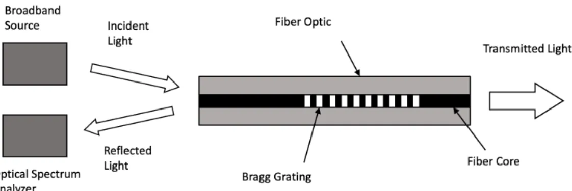
Wavelength modulated sensors use changes of the light wavelength for detection. Fluorescence sensors, black body sensors, and the Bragg grating sensor are examples of wavelength-modulated sensors. Fluorescent based fiber sensors are being widely used for medical applications, chemical sensing and physical parameter measurements such as temperature, viscosity and humidity. The most widely used wavelength based sensor is the Bragg grating sensor. Fiber Bragg gratings (FBGs) are formed by constructing periodic changes in the refraction index in the core of a single mode optical fiber. This periodic change in the refraction index is usually created by exposing the fiber core to an intense interference pattern of UV energy. The variation in refractive index forms an interference pattern that acts as a grating.

(16)

The Bragg grating sensor operation is shown in Figure 1.5, where the light coming from a broadband source (e.g., LED) is sent into the fiber, whose center wavelength is close to the Bragg wavelength. The light propagates through the grating, and part of the signal is reflected at the Bragg wavelength. The complementary part of the process shows a small band of the signal removed from the total transmitted signal. This shows that the Bragg grating is an eﬀective optical filter [2, 7].

1.3.3 Phase Modulated Fiber Optic Sensors

Phase modulated sensors exploit changes in the light phase for detection. The phase of the light, passing through the fiber, is modulated by the field to detect. This phase modulation is then detected interferometrically, by comparing the phase of the light in the signal fiber with that one in a reference fiber. In an interferometer, the light is split into two beams: one is exposed to the external sensing environment that is subjected to a phase shift, while the other one is isolated from the sensing environment and it is used as a reference. Once the beams are recombined, they interfere one with each other [2, 9].

One commonly used interferometer based sensor is the Fiber Fabry-Perot inter-ferometric sensor (FFPI). Fiber guides the incident light into the FFPI sensor and collects the reflected signal from the sensor [2, 10].

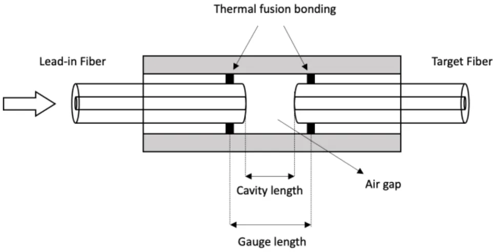
Figure 1.6: Capillary tube based EFPI sensor.

In particular, the Extrinsic Fabry-Perot interferometer (EFPI), represented in Figure 1.6, is made by two cut ends of the fibers with a cavity which acts both as sensing element and waveguide. These two cut ends of the fiber, respectively lead-in and target, are inserted into a glass capillary tube from the opposite parts. Both of them are bond by thermal fusion with the tube. The cavity length between the two fibers is controlled using a precision optical positioner before the thermal fusion bonding. One of the advantages of this EFPI strain sensor is that its gauge length

(17)

and cavity length can be diﬀerent. The strain sensitivity is determined by the gauge length, while the temperature sensitivity is determined only by cavity length since the fiber and tube have the same thermal expansion coeﬃcients. Hence, by making the gauge length much longer than the cavity length, the sensor temperature sensitivity becomes much less than the strain sensitivity. So, no temperature compensation is required.

1.3.4 Polarization Modulated Fiber Optic Sensors

The refractive index of a fiber changes when it undergoes stress or strain, thus it is generated an induced phase difference between different polarization directions. This phenomenon is called photoelastic effect. Moreover, the refractive index of a fiber that is subjected to a certain stress or strain is being defined induced refractive index and it changes by the direction of them. Hence, by detecting the change of the output polarization state, the external perturbation can be sensed.

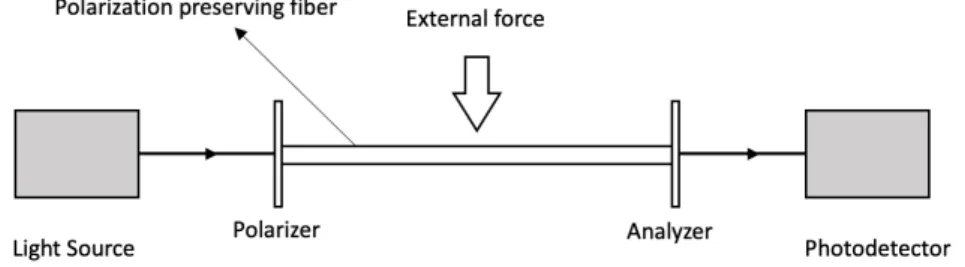
Figure 1.7: Polarization-based fiber optic sensor.

Figure 1.7 shows the optical setup for the polarization-based fiber optic sensor. It is formed by a light source that, through a polarizer, is being polarized at 45 degrees respect to a fiber section, which preserved the polarization; this fiber section acts as sensing fiber [2, 5].

1.4 FBGs Sensor

Because of their small size, immunity to electromagnetic interference, and capability to directly measure physical parameters such as temperature and strain, fiber Bragg grating sensors have developed with time and are becoming a widely used sensing technology.

Although developed initially for the telecommunications industry in the late 1990s, fiber Bragg gratings (FBGs) are increasingly being used in sensing applications. The FBG is an optical filtering device, within the core of an optical fiber, that reflects light of a specific wavelength. The wavelength of light that is reflected depends on the spacing of a periodic variation or modulation of the refractive index inside the core. This grating structure acts as a band-rejection optical filter which accepts all

(18)

wavelengths of light that are not in resonance with it and reflecting wavelengths that satisfy the Bragg condition. This condition, when applied to fiber Bragg gratings, states that the reflected wavelength of light from the grating is B = 2· nef f · ⇤G

where nef f is the eﬀective refractive index seen by the light propagating down the

fiber, and ⇤G is the period of the refractive index modulation of the grating. A

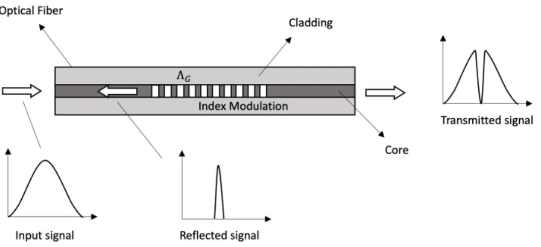
diagram of an FBG is represented in Figure 1.8.

Figure 1.8: Schematic diagram of an FBG having an index modulation of spacing ⇤G inside a single-mode optical fiber.

Typically, the modulation of the core refractive index is created by photo-imprinting a hologram in the photosensitive glass core. It was found that Germanium, which raises the refractive index of silica in the core region of the optical fiber when exposed to high-intensity light, further increases the refractive index of the core itself. By modulating the high-intensity light along the length of the fiber core, it is possible to realize a modulated change in the refractive index of the fiber core. Typically, this spatial modulation is realized by transmitting the UV light through a special transmission diﬀraction grating, so generating a spatial modulation of the light beam that is being photo-imprinted along the length of the core [11].

In other words, when the light is passing through an FBG, one particular wavelength is in phase with the grating period, and this one is reflected back to the input end. All other wavelengths pass through to the other end, since they are not in phase with the grating period. This makes the FBG reflect a particular wavelength and transmit all others. As per Figure 1.8, the first graph is the input spectrum, the second one is the reflected spectrum, and the third one is the transmitted spectrum. Bragg grating wavelength B is the central wavelength that is reflected back by an

(19)

1.4.1 FBGs photo-imprinting in LMA and single-mode fibers

FBG written in single-mode fiber has become one of the most commonly used devices in fiber optic communications, signal processing and optical sensing. Among diﬀerent types of optical fibers, the Large Mode Area (LMA) fibers have been deeply analyzed and developed in order to make it possible to transmit a high-power signal through an optical fiber. These kinds of fibers are characterized by a large core diameter in order to avoid non-linear eﬀects and to guarantee a very low NA which allows to limit the number of modes to a few modes or just the fundamental mode. In particular, singlemode behavior of the LMA fiber is very desirable in the design of high-power fiber lasers since is possible to obtain a high quality output beam [12].

High reflectivity gratings are obtained in this way, achieving respectively 92 % and 93 % for FBG written in LMA fiber and FBG written in single-mode fiber. After many tests, the temperature and strain sensitivity of the LMA fiber FBG were derived and compared with those of the standard single-mode fiber FBG [12].

Before photo-imprinting the FBGs in the optical fibers, their photosensitivity has to be increased. This goal is obtained by highly hydrogen loading, placing them into a chamber with hydrogen at controlled pressure of 130 atm and room temperature.

All gratings are written with photo-imprinting by using the phase-mask technique, in which the phase-mask is exposed to a UV laser beam.

After the photo-imprinting process, the fibers containing FBG are subjected to annealing process by leaving them into an oven for 48 hours at 60 o_{C in order to}

release hydrogen by diﬀusion.

By undergoing LMA fibers and single-mode fibers to strain and temperature changes, it is observed that the temperature coeﬃcients for FBGs written in LMA fiber and standard single-mode fiber are close to each other. The strain coeﬃcient of the FBG inscribed in LMA fiber core is one order of magnitude smaller respect to the FBG written into single-mode fiber. These characteristics show the advantage of FBG written in LMA fibers for temperature sensor applications and, thanks to the robustness of these kinds of fibers, they are very suitable for harsh environments [12, 13].

(20)

Chapter 2 Mechanical Analysis of Fiber Optics

This chapter describes the opto-mechanical properties of fiber optics which, when subjected to deformation, due to the modulation of the refractive index inside the fiber itself, show a coupling between mechanical and optical phenomena. In the next section, the phenomenon is dealt with from a mathematical point of view.

2.1 Opto-Mechanical Model of FBGs

Fiber Bragg gratings (FBGs) are modulations of the index of refraction in optical fibers which act as a wavelength filter. When a Bragg grating is exposed to a broadband spectrum of light, parts of the spectrum at specific wavelengths are reflected. The coupling between the forward and the backward propagating modes results in a resonance condition that occurs at a specific wavelength called Bragg wavelength ( B). The Bragg wavelength is related to the eﬀective refractive index

(nef f) and the period of the refractive index modulation (⇤G).

The Bragg condition can be expressed as

B = 2 nef f⇤G (2.1)

2.1.1 Opto-Mechanical Properties of Optical Fibers

The refractive index in silica, which is a dielectric material, is a function of the applied strain and temperature which, due to photoelastic and thermo-optic eﬀects, cause changes in the refractive index.

Let’s consider a generic volume of dielectric material (⌦) whose temperature and strain distributions are, respectively, T (x, y, z) and "i(x, y, z).

The refractive index of the dielectric, in cartesian coordinates, is expressed as a tensor [n] = 2 4nnxxyx nnxyyy nnxzyz nzx nzy nzz 3 5 (2.2) 11

(21)

Because of the symmetry of the tensor it is possible to rewrite it as [n] = 2 4nn16 nn62 nn54 n5 n4 n3 3 5 (2.3)

In order to define the thermo-optic and photoelastic eﬀects, it is introduced the dielectric impermeability tensor ([B]), whose elements are

Bi= 1 n2 i i = 1, 2, 3 Bi= 0 i = 1, 2, 3 (2.4) Only considering the first-order terms, the variation of impermeability tensor ( Bi),

caused by applied strain and temperature, is given by

Bi = Qi T + pij"j i, j = 1, . . . , 6 (2.5)

where [p] is the strain-optic tensor, called Pockels’ photoelastic constant, ["] is the strain tensor, T is the temperature variation and Qi is a term of temperature

weight.

For an isotropic material [p] is expressed as

[p] = 2 6 6 6 6 6 6 6 6 6 6 4 p11 p12 p12 0 0 0 p12 p11 p12 0 0 0 p12 p12 p11 0 0 0 0 0 0 p11 p12 2 0 0 0 0 0 0 p11 p12 2 0 0 0 0 0 0 p11 p12 2 3 7 7 7 7 7 7 7 7 7 7 5 (2.6)

while the strain tensor ["] is

["] = 2 4""16 ""62 ""54 "5 "4 "3 3 5 (2.7) Qi is defined as Qi= Q0i pij↵j (2.8) where Q0

i is evaluated at constant stress

Q0i= ✓ @ @T ✓ 1 n2 i ◆◆ "=const i = 1, . . . , 6 (2.9) For optically isotropic materials

8 > < > : Q0 i= @ @T ✓ ₁ n2 i ◆ = @ @ni ✓ ₁ n2 i ◆_@n i @T = 2 n3 i @n @T i = 1, 2, 3 Q0 i= 0 i = 4, 5, 6 (2.10)

(22)

where @n

@T is a constant and ↵j is the thermal expansion coeﬃcient which, for an isotropic material, is expressed as

8 > < > : ↵j = ↵ j = 1, 2, 3 ↵j = 0 j = 4, 5, 6 (2.11) By replacing the Eqs.(2.10) and (2.11) into the (2.5), it is obtained

B1= p11"1+ p12("2+ "3) 2 n3 1 ✓_@n @T ◆ T (p11+ 2p12)↵ T B2= p11"2+ p12("1+ "3) 2 n3 2 ✓ @n @T ◆ T (p11+ 2p12)↵ T B3= p11"3+ p12("1+ "2) 2 n3 3 ✓ @n @T ◆ T (p11+ 2p12)↵ T B4= ✓ p11 p12 4 ◆ "4 B5= ✓_p 11 p12 4 ◆ "5 B6= ✓ p11 p12 4 ◆ "6 (2.12)

By linear approximation of Eq.(2.4) it is got Bi = ✓ 1 n2 i ◆ ⇡ _n23 i ni (2.13)

So, it can be rewritten the Eq.(2.12) as n1= n3 1 2 (p11"1+ p12("2+ "3)) + ✓ @n @T ◆ T +n 3 1 2 (p11+ 2p12)↵ T n2= n3 2 2 (p11"2+ p12("1+ "3)) + ✓_@n @T ◆ T +n 3 2 2 (p11+ 2p12)↵ T n3= n3 3 2 (p11"3+ p12("1+ "2)) + ✓ @n @T ◆ T +n 3 3 2 (p11+ 2p12)↵ T n4= n34 ✓ p11 p12 4 ◆ "4 n5= n35 ✓_p 11 p12 4 ◆ "5 n6= n36 ✓ p11 p12 4 ◆ "6 (2.14)

The Eq.(2.14) highlights as the temperature and strain variations induce an optical anisotropy, causing changes in the refractive index.

(23)

2.1.2 Bragg Wavelength Shift Induced by External Stress

and Temperature Variations

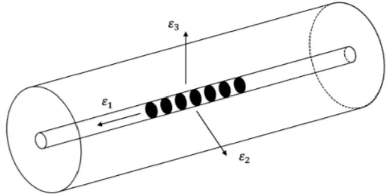
Let’s consider an FBG subjected to a uniform temperature change ( T ) and a strain field with main components "1, "2 and "3, where "1 is the strain component along

the grating direction as shown in Figure 2.1.

Figure 2.1: Fiber Bragg grating subject to strain field.

If "16= "2, there exist two orthogonal guided modes with two eﬀective refractive

indices (nef f,1 and nef f,2).

By replacing n1 and n2, into the Eq.(2.14), respectively with nef f,1 and nef f,2, it

is obtained(1) nef f,1 = n3 ef f,1 2 (p11"1+ p12("2+ "3)) + ✓ @n @T ◆ T + n 3 ef f,1 2 (p11+ 2p12)↵ T nef f,2 = n3 ef f,2 2 (p11"2+ p12("1+ "3)) + ✓ @n @T ◆ T + n 3 ef f,2 2 (p11+ 2p12)↵ T (2.15)

The change of Bragg wavelength in FBGs ( B), is expressed in terms of nef f

and ⇤G variations, under hypothesis of uniform deformations and temperature

variations [16] B = 2 ✓ ⇤G @nef f @l + nef f @⇤G @l ◆ l + 2 ✓ ⇤G @nef f @T + nef f @⇤G @T ◆ T (2.16) which is equivalent to B = 2 (⇤G nef f + nef f ⇤G) _{T =0}+ 2 (⇤G nef f + nef f ⇤G)_"_i₌₀ (2.17)

(1)_{For guided modes, the eﬀective mode index of refraction n}

ef f satisfies ncladding< nef f < ncore.

(24)

where ⇤G = "1⇤G.

By replacing Eq.(2.15) into the (2.17), it is obtained

B1 B = "1 n2 ef f,1 2 (p12"1+ p11"2+ p12"3) + 1 nef f,1 ✓_@n @T ◆ T +n 2 ef f,1 2 (p11+ 2p12)↵ T B2 B = "1 n2 ef f,1 2 (p12"1+ p11"2+ p12"3) + 1 nef f,1 ✓ @n @T ◆ T +n 2 ef f,1 2 (p11+ 2p12)↵ T (2.18)

The reflectivity spectrum of FBGs is splitted into two peaks with Bragg wavelengths

B1 and B2. The Figure 2.2a shows this behaviour, which is called birefringence.

If "2= "3, there is not peak splitting but only a shift of the Bragg wavelength

(Figure 2.2b). The Eq.(2.18) is so modified as follows

B B = "1 n2 ef f 2 (p12"1+ (p11+ p12)"2) + 1 nef f ✓ @n @T ◆ T +n 2 ef f 2 (p11+ 2p12)↵ T (2.19)

Figure 2.2: FBGs reflectivity and the Bragg wavelength shift: (a) diﬀerent trans-verse strain components. (b) equal transtrans-verse strain components.

(25)

Chapter 3 Three-Dimensional Fiber Optics

Shape Reconstruction through FBGs

Array

This chapter deals with the three-dimensional reconstruction of the optical fiber by interpolation, both through the Frenet-Serret equations and through the homoge-neous transformation matrices agorithm. Most of the chapter refers to the article by Paloschi et al. [24], which highlights the advantage of using the second approach for real-time applications. The article is published under the terms of a Creative Commons license which permits use of the content in other media.

The chapter then proceeds with a section dedicated to the implementation of the algorithm on Labview.

3.1 Shape Reconstruction through Frenet-Serret

Equa-tions

3.1.1 Curvature Vector Calculation

The use of FBGs along the fiber for shape detection provides discrete deformation data, such as local position and orientation of the fiber. This discretization in measurements can introduce mathematical errors in the shape reconstruction results. Moreover, the curvature vectors can be determined only at certain points.

The quasi-distributed optical fiber shape detection is based on measurements of the strain of the fiber Bragg grating (FBG). The FBG consists of a periodic modu-lation of the refractive index in the fiber core, which reflects a specific wavelength called the Bragg wavelength ( B), when broadband light is incident on it. This

characteristic wavelength is a function of the period of the grating (the distance be-tween two consecutive high index regions) (⇤B) and of the eﬀective refractive indices

(nef f) of two high index regions, which are modified when mechanical deformation

or temperature is applied to the grating. Furthermore, multiple FBGs (i.e., FBG arrays) with diﬀerent gratings periods can be used along the same fiber to have a quasi-distributed strain measurement. The high sampling rates (up to 10 kHz) and

(26)

lower costs of interrogation devices for FBG measurements make quasi-distributed shape detection more suitable for real-time applications [24].

It is considered a multi-core fiber (MCF), constituted by three cores located at the vertices of an equilateral triangle, whose cross-section is shown in Figure 3.1 [22].

Figure 3.1: Multi-core fiber cross-section view at F BGi and parameters for

curva-ture calculation.

In order to calculate the curvature under bending deformation, it is considered the partial curvature vectors for each i-th side core

i=

1 rc

("icos ↵inx+ "isin ↵iny) (3.1)

where rc is the distance between the centers of the fiber and the core, "i is the strain

associated with a length change, ↵i is the angle between the direction to the core

and the local x-axis, nx and ny are unit vectors for the x and y axes, respectively.

The relationship between the strain ("i) and the Bragg wavelength shift ( i)

can be obtained from the following equation [23]

i B i

= Ci"i+ ⌦dT (3.2)

where, considering the i-th side core, B

i is the Bragg wavelength at initial conditions

(no strain applied), Ci = 1 pi is the strain coeﬃcient, determined during calibration

process, pi is the strain-optic coeﬃcient, ⌦ is the temperature sensitivity, and T is

the temperature. Without considering for now the temperature dependence, the strain values "i are obtained by analyzing the shifts in Bragg wavelengths of spectra,

reflected from the gratings [24]

"i= 1 Ci i B i (3.3)

(27)

Since the central core of a multi-core fiber is not subjected to bending-induced strain, the Bragg wavelength shifts of the FBGs in this core have to be subtracted from the wavelength shifts of the FBGs in the side cores, in order to compensate the eﬀect of longitudinal strain and temperature on the calculated curvature.

Moreover, in order to achieve more accurate results, the strain data are inter-polated with the cubic Hermitian function, whose interpolation coeﬃcient (m) will be used to indicate the number of additional segments in which the span between two consecutive FBGs is furtherly divided. With respect to spline interpolation technique, which is smoother and more accurate if the data represents values of a smooth function, the cubic Hermite interpolation has no overshoots and gives a result with less oscillations [24].

The curvature vector  is then calculated from the strain values with the following formula  = 2 N rc N X i=1 "icos ↵inx+ N X i=1 "isin ↵iny ! (3.4) where N is the number of cores, rc is the core distance from the fiber center, nx and

ny are the unit vectors that define the plane where the FBG triplet lies and ↵i is

the angle between nx and the i-th core, as shown in Figure 3.1.

Curvature radius R and curvature angle ✓ are calculated, from the curvature vector , as

R = 1

kk (3.5)

✓ = angle() (3.6)

3.1.2 Frenet-Serret Frame

A curve in the three-dimensional space can be defined by Frenet-Serret equations [25]

r0(u) = T (u) T0(u) = (u)N (u) N0(u) = ⌧ (u)B(u) (u)T (u)

B0(u) = ⌧ (u)N (u)

(3.7)

where u is the coordinate along the fiber and r(u) is the poistion vector. T (u), N(u) and B(u) are, respectively, tangent unit vector, normal unit vector and binormal (calculated as cross-product of T (u) and N(u), which lie in the osculating plane). The scalar functions ⌧(u) and (u) are the torsion and the curvature of the shape [22, 24].

By considering to divide the entire length in sub-parts having length equal to s, and indicating the position of a specific virtual F BGi according to the index i, the

(28)

Eq.(3.7) can be rewritten in a discrete form r(i) r(i 1) s = T (i) T (i) T (i 1) s = (i)N (i) N (i) N (i 1)

s = ⌧ (i)B(i) (i)T (i) B(i) B(i 1)

s = ⌧ (i)N (i)

(3.8)

which, in order to be more easily implemented in a code (i.e. MATLAB), can be mathematically manipulated as

N (i) = s⌧ (i)B(i 1) s(i)T (i 1) + N (i 1) 1 + s2_⌧2_{(i) + s}2_2_(i)

T (i) = s(i)N (i) + T (i 1) B(i) = s⌧ (i)N (i) + B(i 1)

r(i) = sT (i) + r(i 1)

(3.9)

The Frenet-Serret equations assume the length of a span to be infinitesimal (i.e. s! 0) and the curve to always be well defined (curvature radius R < 1) so that the frame {T, N, B} can be univocally defined. An infinitesimal s can be achieved with a suﬃciently large interpolation factor (m), making shorter the distance between two consecutive FBGs. On the other hand, it cannot be always guaranteed that a curvature exists in certain points (e.g., inflection points) [24].

3.2 Homogeneous Transformation Matrices Algorithm

3.2.1 Description of Algorithm

This kind of algorithm is based on fiber optics shape reconstructing by using homogeneous transformation matrices, through which it is possible to express the position of a certain point at diﬀerent frames well-defined along the fiber.

(29)

Figure 3.2: F BGi section view, {xi, yi} plane.

F BGi senses a curvature radius Ri and an azimuth angle ✓i, which identify an

in-plane rotation center ci.

As per Figure 3.2, the first step consists in a rotation of the i-th frame {xi, yi, zi}

(corresponding to the virtual F BGi) around the zi-axis, of the azimuth angle ✓i, in

order to align the x-axis with the curvature center ci. The rotation matrix is

Rzi(✓i) =

2

4sin(✓cos(✓ii)) cos(✓sin(✓i)i) 00

0 0 1

3

5 (3.10)

In order to express the position of the F BGi+1 with respect to F BGi it is

necessary to describe a circular path of length s (i.e. FBG distance) around center ci. Referring to the Figure 3.3, the angle 'i is obtained from the known parameters

Ri and s, and is used to re-align the x-axis towards the rotation center ci.

Figure 3.3: Multicore fiber, external side view, {x0

(30)

The rotation of the frame {x0

i, y0i, zi0} is expressed by the matrix

Ry0 i('i) = 2 4 cos('0 i) sin('1 i) 00 sin('i) cos('i) 0 3 5 (3.11)

The next step is to express the frame {T00_{} = {x}00

i, y00i, zi00}, centered at the

position F BGi, with respect to F BGi+1 (Figure 3.4).

Figure 3.4: Location of oi+1 from oi

The position of oi+1 with respect to oi, in the plane {x0i, zi0}, is represented by

the vector oi i+1({x0i, zi0}) = " Ri(1 cos('i)) Risin('i) # (3.12) Instead, the projection of the position oi+1, with respect to oi in the plane {xi, yi}

is described by the vector

oii+1({xi, yi}) = " Ri(1 cos('i)) cos(✓i) Ri(1 cos('i)) sin(✓i) # (3.13) By merging these last two equations, one obtains the origin of frame i + 1 with respect to frame i oii+1 = 2 6 4 Ri(1 cos('i)) cos(✓i) Ri(1 cos('i)) sin(✓i) Risin('i) 3 7 5 (3.14)

In order to determine the position of the F BGi+1 with respect to the F BGi, it

is introduced the homogeneous transformation matrix (Ai

i+1) from frame i + 1 to

frame i, which is obtained by merging the Eqq.(3.10),(3.11) and (3.14) ˜

pi

i+1 = Aii+1p˜i+1i+1 = =

" Rzi(✓i)Ryi0('i) o i i+1 0T 3 1 # ˜ pi+1 i+1 (3.15)

(31)

where ˜pi

i+1 is the vector of the homogeneous coordinates of F BGi+1 with respect

to the reference frame located at F BGi and ˜pi+1i+1 is the vector of the homogeneous

coordinates of F BGi+1 with respect to itself.

The complete inner structure of the homogenous transformation matrix is

Aii+1 = 2 6 6 6 6 4

cos(✓i) cos('i) sin(✓i) cos(✓i) sin('i) Ri(1 cos('i)) cos(✓i)

sin(✓i) cos('i) cos(✓i) sin(✓i) sin('i) Ri(1 cos('i)) sin(✓i)

sin('i) 0 cos('i) Risin('i)

0 0 0 1 3 7 7 7 7 5 (3.16) This change of coordinates will be applied during the shape reconstruction to express all the FBG positions in the starting frame. By multiplying the homogenous matrices, which express the frame of the virtual F BGi with respect to the previous one, it is

obtained

˜

p0_i+1 = A0₁A1₂_{· · · A}i 1_i Ai_i+1p˜i+1_i+1= A0_i+1p˜i+1_i+1 (3.17)

3.2.2 Description of Labview Code for Real-time

Applica-tions

The algorithm described in section 3.2.1 has been developed in Labview environment, in order to use it for real-time applications.

First of all, it is necessary to define the length of the virtual subdivisions (s), calculated as (Figure 3.5)

s = L

(NF BG 1)m (3.18)

where L is the total length of the optical fiber, NF BG is the number of real FBGs

(so NF BG 1 is the number of segments) and m is the interpolation coeﬃcient.

Figure 3.5: Calculation of s starting from the total length of the fiber optic, number of real FBGs and interpolation coeﬃcient.

Cubic Hermite interpolation is more suitable for this purpose, as it has no overshoots and yields a result with less oscillations with respect to the spline interpolation.

(32)

Figure 3.6: Cross-section of j-th node. The side-cores are core a, core b and core c. The central one (core 0 ) is used for temperature compensation.

According the Figure 3.6, the wavelength shifts are detected from the four cores of the fiber optic. For what concerns the central core (i.e. core 0 ), it is not subjected to bending-induced strain and its function is just to compensate the eﬀect of longitudinal strain and temperature on the calculated curvature.

Hence, for this reason, its wavelength shifts have to be subtracted to the side-cores wavelelength shifts (Figure 3.7).

By considering the j-th node

a= a,T 0

b= b,T 0

c= c,T 0

(3.19)

where a,T, b,T and c,T are the side-cores wavelelength shifts before

tempera-ture compensation.

Figure 3.7: Calculation of of the cores, by taking into account temperature compensation.

The Eq.(3.3) allows to compute, per FBG, the strain vector (") starting from wavelength shift vector ( ), reference Bragg wavelength vector ( B) and strain

(33)

coeﬃcient vector (Figure 3.8) "a,j = 1 Ca,j a,j B a,j "b,j = 1 Cb,j b,j B b,j "c,j = 1 Cc,j c,j B c,j for j = 1, . . . , 6 (3.20)

Figure 3.8: SubVI.vi for strain calculation: the block is made up of a for loop, in which the deformations are calculated for a certain number of iterations as many as the number of the FBGs.

After this computation, as said before, one has to performs shape-preserving cubic Hermite interpolation, as shown in Figure 3.9, 3.10 and 3.11

(34)

Figure 3.10: SubVI.vi for Hermitian interpolation of the strain vectors: x is the ramp vector from 1 to 6, whose dimension is equal to 6; xq1 is the ramp vector from

1 to 6, whose dimension is equal to 501.

Figure 3.11: SubVI.vi for Hermitian interpolation of the strain vectors: the Hermite Interpolation 1D.vi block receives x, ✏ and xq1 vectors, in order to calculate the

output vectors of interpolated values.

The curvature vector  is then calculated from the Eq.(3.21)  = 2 3r 3 X k=1 "kcos ↵knx+ 3 X k=1 "ksin ↵kny ! = = 2

3r("acos 0 nx+ "asin 0 ny+ "bcos 120 nx+ +"bsin 120 ny+ "ccos 240 nx+ "csin 240 ny)

(3.21)

where the number of cores is equal to 3 for the case under examination, r is the core distance from the central one, nx and ny are the unit vectors that define the plane

(35)

This calculation has been developed in Labview environment by using a while loop structure in order to build the i for i = 1, . . . , length("H), where "H is the

strain vector after Hermitian interpolation (Figure 3.12).

Figure 3.12: SubVI.vi for computation of curvature radius: R = 1

kk and azimuth angle: ✓ = angle(kk).

The next step of the algorithm consists in the calculation of the rise angle (') and the variation of the azimuth angle (d✓).

As per Figure 3.4, the rise angle is obtained from the geometry of the fiber 'i =

s Ri

180

⇡ (3.22)

while the azimuth angle variation is

d✓i= ✓i ✓i 1 (3.23)

These two calculations have been developed in Labview, as shown in the Figure 3.13

Figure 3.13: SubVI.vi for calculation of the rise angle (') and the variation of the azimuth angle (d✓).

After this calculation, it is necessary to initialize the rotation matrices, which preoviously have been introduced, in order to compute the initial homogeneous

(36)

transformation matrix. In order to do that, it is necessary to implement the following formulas in the Labview code (Figure 3.14).

Rzi(✓0) =

2

4cos(✓sin(✓00)) cos(✓sin(✓00)) 00

0 0 1 3 5 (3.24) Ry0 i('0) = 2 4 cos('0 0) sin('1 0) 00 sin('0) cos('0) 0 3 5 (3.25)

The initial position is

p0= 2 6 4 0 0 0 3 7 5 (3.26)

So the homogeneous transformation matrix is (see Eq.(3.27)) A0= " Rzi(✓0)Ry_i0('0) p0 0T 3 1 # (3.27)

Figure 3.14: SubVI.vi for computation of the initial homogeneous transformation matrix.

A0 is necessary for the calculation of An0, according the Eq.(3.17)

˜

(37)

where n is the dimension of the position vectore, and ˜p0

n is the homogeneous

coordinates vector of the last n-th virtual FBG with respect to the initial position p0.

The computation of the position vector is performed by the SubVI (Figure 3.15), which contains a while loop structure, in order to build the position vector pi per

each index i

Figure 3.15: SubVI.vi for calculation of the position array, in homogeneous coordinates, and extraction of the px, py and pz components in order to obtain a 3D

plot.

By using an event structure inside a case structure it is possible to have a real-time plot. Thanks to this, each time the input vectors of wavelength shift ( a,

b and c) change their values, the plot is re-initialized and the previous one is

(38)

Figure 3.16: The event structure modifies the status each time an event occurs. The case structure receives the change of state as input and based on this the instruction to be executed.

Figure 3.17: Labview front panel: the position array describes the location of the end-tip in the (x, y, z) frame; the delta array contains the initial values of the wavelength shifts, and delta mod contains the updated ones; the stop button stops the acquisition of the signal and re-initializes all the values.

(39)

3.3 Comparison between Frenet-Serret Equations

and Transformation Matrices Algorithm

In order to better understand the behaviour of the two methods, some experiments have been done. This section takes into account numerical values and setup, used for the experiments reported in the article of Paloschi et al. [24].

In order to evaluate the performances of the two approaches, it was used a polymide-coated 7-core optical fiber containing 3D FBG arrays (they were manu-factured by the Fiber Optics Research Center, in Moscow). The fiber has seven identical straight cores – the central one and six surrounding side cores located in the corners of a regular hexagon, as per Figure 3.18. The distance between the cores is 40.5 µm, the cladding diameter is 125 µm, and the mode field diameter for each core is 5.7 µm at 1550 nm and the coating polymide layer has a thickness of 15 µm. The polyimide protective coating of the fiber provides a high mechanical strength and a high-temperature resistance, making this sensor well-suited for harsh environments or for some medical and composite material applications.

Figure 3.18: Multicore fiber. Schematic representation of a 3D FBG array inscribed in the polyimide-coated 7-core optical fiber: a) 3D view and b) cross-section.

In each node, uniform FBGs with a constant length LF BG= 2 mmwere inscribed

in the central core, and in three side cores located at the corners of an equilateral triangle, so the fiber optic total length is 72 mm.

To interrogate the fabricated multicore fibers, it was used the HBM FS22-SI 8-channel interrogation unit (wavelength range from 1500 nm to 1600 nm, Figure 3.19).

(40)

Figure 3.19: Measurement system. Interrogation scheme used for FBG resonances detection and tracking.

The shape reconstruction was performed for diﬀerent setups. In this section, it will be discussed about one of them (for the other ones, take reference to [24]).

The reconstruction is iterated for both methods, plotting the average error as a function of the increasing interpolation factor m (Figure 3.20). The best achievable average error is 0.28 mm.

Figure 3.20: Shape reconstruction, average error - the average distance between the points calculated by the two diﬀerent algorithms with the same interpolation factor and the ground truth is presented. As the interpolation factor is increased, the diﬀerence becomes negligible.

In order to represent the 3D shape reconstruction, it was chosen a fixed valure of the interpolation factor: m = 100 (Figure 3.21).

(41)

Figure 3.21: 3D shape reconstruction - ground truth (solid line), recovered shape with the proposed method (dashed black line) and recovered shape with Frenet-Serret (dashed red line) are shown. The chosen interpolation factor is m = 100 as it provides a trade-oﬀ between accuracy and performance [24].

As it can be inferred from the experiments the reconstruction error for Frenet-Serret tends to the same value of the transformation matrices for increasing values of interpolation factor (m).

Moore et al. obtained discrete strain measurements from each core to create a continuous representation of the curvature and twist of the fibers. The Frenet-Serret equations are then resolved to obtain the shape of the fiber. The shape measurements were found to have a maximum estimated error around 7.2%, and the main cause of this error could be an externally induced twist in the fiber. Future work will focus on eliminating this error by including torsion measurements into the shape solution [26].

Paloschi et al. estimated that the main source of error by using Frenet-Serret method is most likely the computational eﬀort needed to perform the satisfactory level of interpolation on the data. On the other hand, the homogeneous transformation matrices algorithm is not sensible to discontinuities in the phase and performs well even at low values of interpolation [24].

Roesthuis et al. used two models to predict the needle shape when inserted into a soft tissue: the first one is a kinematics-based model which considers needle deflection considering constant-curvature segments after each needle rotation. The second model is a mechanics-based model which predicts needle deflection based on needle-tissue interaction forces.

For what concerns the current needle shape, they estimated that errors in the reconstructed shape become larger for complex deflections (i.e., multiple bends and out-of-plane bending). These errors are both dependent on the needle curvature approximation technique, because the position of the FBG sensors are not constant during bending and this causes errors in the calculated needle curvature, and on the use of a linear spline interpolation technique, because of the limited number of FBG sensors.

Instead, for what concerns the models which provide information about the predicting 3D path for a flexible needle during insertion into a soft tissue, Roesthuis

(42)

obtained the following results: the mechanics-based model has shown to predict the needle shape more accurately for the out-of-plane insertion case, with respect to the kinematics-based model. Nevertheless, the kinematics-based model is preferred for real-time applications (e.g., needle steering) because of the ease of implementation.

In order to predict the needle shape using the kinematics-based model, more investigation is required about the curvature radius and cut angle when the needle bends out-of-plane [21].

(43)

Conclusion

This work presents the algorithm based on the estimation of the real-time three-dimensional reconstruction of multicore optical fibers subjected to deformation, by using the Labview software. Multicore fibers allow accurate measurement of their shape, making them suitable for those applications where accuracy is the main goal. Among the main fields of interest for the application are medical and industrial robotics, mining and aerospace industries.

The algorithm based on transformation matrices is characterized by a better performance than the traditional Frenet-serret equations, showing to be suitable for applications that require a very good accuracy in a very short time or in real-time. In fact, it is able to provide the same accuracy with fewer interpolations, while being less sensitive to discontinuities in the values of the measured angles of curvature.

Future work will involve some changes to the implemented code, further reducing the computational cost and ensuring optimal results.

(44)

Bibliography

[1] Frank L. Pedrotti, Leno S. Pedrotti, Leno M. Pedrotti, Introduction to Optics, Pearson Internetional Edition, Third Edition, 2007.

[2] Fidanboylu, K., Efendioğlu, H.S., “Fiber optics sensors and their applications”, 5th International Advanced Technologies Symposium (IATS’09), Karabuk, Turkey, May 13-15, 2009.

[3] O. Svelto, “Fisica delle Fibre Ottiche”, Politecnico di Milano, 2007.

[4] Jones, D., “Introduction to Fiber Optics”, Naval Education and Training Professional Develeopment and Technology Center, 1998.

[5] Yu, F. T. S., and Shizhuo, Y., “Fiber Optic Sensors”, Marcel Decker, Inc., Newyork, 2002.

[6] Casas J. R., and Paulo, J. S., Fiber Optic Sensors for Bridge Monitoring, Journal of Bridge Engineering, ASCE, 2003.

[7] Méndez, A., “Overview of fiber optic sensors for NDT applications”, IV NDT Panamerican Conference, 1-11, 2007.

[8] Berthold, J. W., “Historical Review of Microbend Fiber Optic Sensors”, Journal of Lightwave Technology, Vol. 13, 1193-1199, 1995.

[9] Krohn, D. A., “Fiber Optic Sensors: Fundamental and Applications”, Instru-ment Society of America, Research Triangle Park, North Carolina, 1988. [10] Wang, Z., “Intrinsic Fabry-Perot Interferometric Fiber Sensor Based on

Ultra-Short Bragg Gratings for Quasi-Distributed Strain and Temperature Measure-ments”, M.S. Thesis, Virginia Tech, 2003.

[11] S. J. Mihailov, “Fiber Bragg Grating Sensors for Harsh Environments”, Sensors, 12, 1898-1918, 2012.

[12] I. R. Ivascu, R. Gumenyuk, S. Kivistö, O. G. Okhotnikov, “Characterization of Fiber Bragg Gratings Written in Large Mode Area Fibers”, UPB Scientific Bulletin, Series A: Applied Mathematics and Physics, Vol. 73, Iss. 4, 2011. [13] R. Paschotta, “Large Mode Area Fibers” in the Encyclopedia of Laser

Physics and Technology, Wiley-VCH, ISBN 978-3-527-40828-3, First Edition, October 2008.

(45)

[14] H. Alemohammad (Ed.), Opto-Mechanical Fiber Optic Sensors: Re-search, Technology, and Applications in Mechanical Sensing, Elsevier: Amsterdam, The Netherlands, 2018.

[15] Udd, E., W. Schulz, J. Seim, J. Corones, and H. M. Laylor, “Fiber Optic Sensors for Infrastructure Applications”, Oregon Department of Transportation, Washington D.C, 1998.

[16] Othonos A., Kalli K., Fiber Bragg Gratings, Boston: Artech House, First Edition, 1999.

[17] R. J. Roesthuis, M. Kemp, J. J. van den Dobbelsteen, and S. Misra, “Three-Dimensional Needle Shape Reconstruction Using an Array of Fiber Bragg Grating Sensors”, IEEE/ASME Transactions on Mechatronics, Vol. 19, no. 4, August 2014.

[18] Y. L. Park, S. Elayaperumal, B. Daniel, S. C. Ryu, M. Shin, J. Savall, R. Black, B. Moslehi, and M. Cutkosky, “Real-time estimation of 3-D needle shape and deflection for MRI-guided interventions,” IEEE/ASME Trans. Mechatronics, Vol. 15, no. 6, pp. 906–915, Dec. 2010.

[19] K. Henken, D. van Gerwen, J. Dankelman, and J.J. van den Dobbelsteen, “Ac-curacy of needle position measurements using fiber Bragg gratings,” Minimally Invas. Therapy Allied Technol., Vol. 21, no. 6, pp. 408–414, 2012.

[20] V. Duindam, R. Alterovitz, S. Sastry, and K. Goldberg, “Screw-based motion planning for bevel-tip flexible needles in 3-D environments with obstacles,” in Proc. IEEE Int. Conf. Robot. Autom., pp. 2483–2488, Pasadena, CA, USA, May 2008.

[21] R. J. Roesthuis, M. Abayazid, and S. Misra, “Mechanics-based model for pre-dicting in-plane needle seflection with multiple bends,” in Proc. IEEE/EMBS Int. Conf. Biomed. Robot. Biomechatron., pp. 69–74, Rome, Italy, Jun. 2012. [22] K. Bronnikov et al., “Durable shape sensor based on FBG array inscribed

in polyimide- coated 7-core optical fiber” Opt. Express, Vol. 27, no. 26, pp. 38421–38434, 2019.

[23] C. D. Butter and G. B. Hocker, “Fiber optics strain gauge”, Appl. Opt., AO 17(18), 2867–2869, 1978.

[24] Paloschi, D., Bronnikov, K. A., Korganbayev, S., Wolf, A., Dostovalov, A., Saccomandi, P. (2020). 3D shape sensing with multicore optical fibers: trans-formation matrices vs Frenet-Serret equations for real-time application. IEEE Sensors Journal.

[25] A. T. Fomenko and A. S. Mishchenko, A Short Course in Diﬀerential Geometry and Topology, Cambridge Scientific Publishers, 2009.

[26] J. P. Moore, M. D. Rogge, “Shape sensing using multi-core fiber optic cable and parametric curve solutions”, Optics express, 20(3), 2967-2973, 2012.

3D reconstruction of the shape of optical fibers subjected to mechanical deformations

School of Industrial and Information Engineering

MSc Mechanical Engineering - Mechatronics and Robotics