Ecological modelling of the phytoplankton dynamics in the northern Gulf of Aqaba (Red Sea)

(1)

ALMA MATER STUDIORUM

UNIVERSITA' DI BOLOGNA

FACOLTA' DI SCIENZE MATEMATICHE FISICHE E NATURALI

Corso di laurea magistrale in BIOLOGIA MARINA

“Ecological modelling of the phytoplankton dynamics in the northern

Gulf of Aqaba (Red Sea)”

Tesi di laurea in Evoluzione ed Adattamenti degli Invertebrati Marini

Relatore

Presentata da

Dr. Stefano Goffredo Leonardo Laiolo

(Università di Bologna)

Correlatori

Dr. Alberto Barausse (Università di Padova)

Prof. Luca Palmeri (Università di Padova)

Dr. David Iluz (Bar-Ilan University, Israele)

Prof. Zvy Dubinsky (Bar-Ilan University, Israele)

I sessione

(2)

(3)

“The sciences do not try to explain, they hardly even try to interpret, they mainly make models. By a model is meant a mathematical construct which, with the addition of certain verbal interpretations describes observed phenomena. The justification of such a mathematical construct is solely and precisely that it is expected to work”

(4)

(5)

ABSTRACT

The Gulf of Aqaba represents a small scale, easy to access, regional analogue of larger oceanic oligotrophic systems. In this Gulf, the seasonal cycles of stratification and vertical mixing drive the annual phytoplankton dynamics and patterns. In summer and fall, when nutrient concentrations are very low, Prochlorococcus and Synechococcus are more abundant in the surface waters. At that time these two populations are exposed to phosphate limitation. During winter mixing, when nutrient concentrations are higher,

Chlorophyceae and Cryptophyceae become dominant but are scarce or

absent during summer.

In this study it was tried to develop a simulation model based on historical data to predict the phytoplankton dynamics in the northern Gulf of Aqaba. The purpose is to understand what forces operate, and how, to control the phytoplankton dynamics in the Gulf.

For the models data sampled in two different sampling station (Fish

Farm Station and Station A) were used, concomitant with data of chemical,

biological and physical factors, from 14th January 2007 to 28th December 2009. The Fish Farm Station point was near a Fish Farm that was operational until 17th June 2008, the complete closure date of the Fish Farm, about halfway through the total sampling period. The Station A sampling point is about 13 km away from the Fish Farm Station. To build the model, the MATLAB software package was used (version 7.6.0.324 R2008a), in particular a tool named Simulink.

The Fish Farm Station models shows that the Fish Farm activity has altered the nutrient concentrations and as a consequence affected the normal phytoplankton dynamics. Despite the considerable distance between the two sampling stations, there might be some influence from the Fish Farm activities also on the Station A ecosystem. The models of this sampling station show that the Fish Farm impact appears to be much lower than in the Fish Farm Station, because the phytoplankton dynamics at Station A appear to be driven mainly by the seasonal mixing cycle.

(8)

2

INTRODUCTION

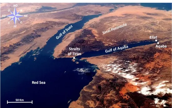
DESCRIPTION OF THE ECOSYSTEM

The Gulf of Aqaba is one of two large gulfs in the Red Sea, located to the east of the Sinai Peninsula and west of the Arabian mainland, separated from the Red Sea by the 252 m deep sill at the Straits of Tiran (Fig. 1). This Gulf is 170 km long and 14-24 km wide, with an average depth of 800 meters and a maximum of 1830 meters. For these reasons the Gulf of Aqaba represents a small scale, easy to access, regional analogue of larger oceanic oligotrophic systems (Chen et al. 2008).

Fig. 1:Gulf of Aqaba with the position of Eilat (Israel) and Aqaba (Jordan)

In the Gulf of Aqaba the climate is extremely arid, the yearly precipitation at the northern gulf averages only 30 mm, and hot, with summer air temperature reaching up to 45°C, with prevailing northerly winds. Excess evaporation over this minimal precipitation is in the range of 2000 mmy-1 (Monismith et al. 2006). No rivers flow into the gulf, and fresh water, other than rain, reaches it only occasionally during rare winter floods.

The two largest cities in this area are Eilat (Israel) and Aqaba (Jordan), these cities rise in front of a coral reef that supports a complex and fragile ecosystem. Southern Eilat, where the nature reserve "Coral Beach" was set up in 1974, encompasses the northernmost coral reef in the world.

(9)

3

The coral reef stretches over 1200 metres along the west coast of the Bay of Eilat and inspite of its marginal position as a coral reef, it has more than 1000 different species of corals and accommodates a wide biodiversity of fish species and invertebrates, including several endemic species. The coral reef, in front of the city of Eilat and Aqaba, supports a thriving economy based primarily on tourism. Environmental factors might threaten this important source of revenue; in particular some studies show a worsening of sea-water quality due to human activity and industrial pollution in the coastal zones surrounding the Gulf: metallurgical industries, hotels and resorts, port activities and fish farming (Chen Y et al. 2008, Lazar B et al. 2008, Loya Y et al. 2003, Loya Y et al. 2004). Global climate change may also be a contributory factor: the dust deposit in the Gulf due to desertification processes, water warming and acidification caused by an anthropogenic increase in atmospheric greenhouse gases, and increase in UV radiation due to ozone depletion (Lazar B et al. 2008, Chen Y et al. 2007, Chen Y et al. 2008). A combination of these factors may play a role in deteriorating reef conditions.

This area is dominated by mineral dust deposition and surrounded by deserts; anthropogenic air emissions may make a significant contribution to the level of various trace of elements such as Cu, Cd, Ni, Zn (Chen et al. 2008). Relative isolation from the main Red Sea and the Indian Ocean, intense solar radiation for most of the year, low plankton biomass, and low POM (Particulate Organic Matter) characterize the Gulf of Aqaba. The low levels of nitrogen and phosphate nutrients are the main limiting factors in the Gulf of Aqaba (Al-Qutob et al. 2002, Labiosa et al. 2003). In recent years it has been seen that the atmospheric inputs of other nutrients gradually increase the likelihood of P limitation in the Gulf (Chen et al. 2007). As a result of these studies it has been recognized that P limitation in the ocean may be more prevalent than previously estimated, and that the efficiency of P uptake among individual groups of phytoplankton may, in fact, control the phytoplankton species composition observed in a given community. Furthermore, it has been suggested that a transition from N limitation to P limitation has taken place over the last two decades in the

(10)

4

North Pacific Subtropical Gyre, and that this favours the growth of

prokaryotic picophytoplankton, such as Prochlorococcus and

Synechococcus, which have a large surface area to volume ratio and take up

nutrients more efficiently than larger phytoplankton (Karl et al. 2001).

SEASONAL CYCLES OF STRATIFICATION AND MIXING

The Gulf of Aqaba has similar seasonal cycles of stratification and mixing to other subtropical oligotrophic seas. Small perturbations such as transient cooling (that induces convection) and wind events (that drive upwelling) can at times inject deep water to the surface euphotic layer, making nutrients available for phytoplankton growth (Labiosa et al. 2003). When the mixing layer exceeds a critical depth phytoplankton bloom cannot develop (Sverdrup 1953).

The water column of the northern Gulf of Aqaba is stratified during summer, and, under normal conditions, surface water nutrient levels are near the limits of detection (Levanon-Spanier et al. 1979, Mackey et al. 2007). During the summer months atmospheric dry deposition is a significant source of nutrients to the euphotic zone, supporting transient phytoplankton blooms (Chen et al.2007, Paytan et al. 2009). Beginning in the fall, cooling of surface waters initiates a convective mixing, and a deeply mixed (300 meters or more) water body is observed by winter (Wolf-Vetch et al. 1992). During winter and early spring the convective component of entrainment is strong enough to mix the surface waters below the critical depth as well as bring large quantities of the nutrients to the surface (Labiosa et al. 2003). The water column begins to re-stratify in the spring as surface waters warm, trapping nutrients and phytoplankton in the euphotic zone along a steep light gradient.

SEASONAL PHYTOPLANKTON DYNAMICS

The nature of the seasonal phytoplankton dynamics may have important implications for trophic interactions within the Gulf of Aqaba (Labiosa et al. 2003). The phytoplankton bloom will have consequences for the food web, consisting of a stronger temporal decoupling between

(11)

5

phytoplankton and zooplankton dynamics (Tagliabue and Arrigo 2003). It has also been shown that the productive coral reefs in the Gulf of Aqaba subsist, for their nutrient supply, to a large degree on allochthonous plankton with nitrogen fluxes from the phytoplankton to the coral reef (Yahel et al. 1998, Richter et al. 2001). In the absence of a significant phytoplankton bloom, phytoplankton may become too scarce to support coral reef production. Therefore, the interannual variability in the intensity and timing of phytoplankton blooms may have serious consequences for the upper trophic levels in the Gulf of Aqaba (Labiosa et al. 2003). Phytoplankton patterns were shown to follow the seasonal hydrological cycle in the Gulf of Aqaba (Iluz et al. 2008).

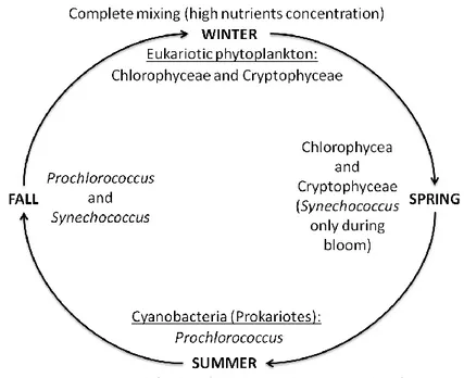
During winter the Gulf of Aqaba is subjected to benthic injections of nitrogen that maintain the nitrogen phosphorus ratio close to the ―Redfield Ratio‖ (Häse et al. 2006). At this time, eukaryotic algae dominate but their growth rate is limited by light availability with deep mixing (Lindell and Post 1995, Stambler 2005, Al-Najjar et al. 2007). In particular

Chlorophyceae and Cryptophyceae are dominant during winter mixing but

scarce or absent during summer (Fig. 2) (Al-Najjar et al. 2007). Water column stratification and the development of the thermocline initiated during spring, entraps nutrients in the high-light surface water resulting in phytoplankton blooms, typically cyanobacteria and diatoms (Lindell and Post 1995, Al-Najjar et al. 2007, Suggett et al. 2009). In particular

Synechococcus was the main component of phytoplankton during a wind

triggered spring bloom of massive proportions (Iluz et al. 2008, Suggett et al. 2009). As spring progresses into summer, the phytoplankton community becomes increasingly dominated by picoeukaryotes and prochlorophytes (Lindell and Post 1995, Al-Najjar et al. 2007, Stambler 2006). Stratification minimizes deep-water injections of nitrogen into near-surface waters, and atmospheric loading of nutrients becomes an important determinant of nutrient availability (Chen et al. 2007).

In summer and fall, when nutrient concentrations are very low, picophytoplankton (cells <2µm) (Prochlorococcus and Synechococcus) are more abundant in the surface water; in particular Prochlorococcus was the

(12)

6

main component of the community during summer stratification (Fig. 2) (Lindell and Post 1995, Post et al. 1996, Mackey et al. 2007). Typically picophytoplankton account for about 37% of phytoplankton cells in winter, whereas they account about 84% of cells in summer and fall, increasing in relative abundance as stratification progresses and nutrients become scarce (Mackey et al. 2007). During summer Prochlorococcus and Synechococcus populations in the Gulf of Aqaba are exposed to phosphate limitation (Fuller et al. 2005, Mackey et al. 2009).

Fig. 2: The seasonal cycle of stratification and mixing and the phytoplankton constituting

the majority of the total chlorophyll a for each season.

AIM OF THIS STUDY

The aim of this study is to develop a simulation model based on historical data to predict the phytoplankton dynamics in the northern Gulf of Aqaba. The purpose is to understand what forcing functions operate, and how, to control the phytoplankton dynamics in the northern Gulf of Aqaba.

This model might signal deterioration of the waters in front of Aqaba and Eilat due to the Fish Farm activity. This will provide decision-makers with a tool to evaluate the cost/benefit effectiveness of legislative measures under various local developments and global climate change scenarios and to assist in the prevention of potentially detrimental activities. The model

(13)

7

will be useful for future predictions on the environmental conditions in the Gulf of Aqaba and any corrective measures to protect unique high biodiversity of the sensitive ecosystems of the Gulf.

(14)

8

MATERIALS AND METHODS

SAMPLING AND INSTRUMENTS USED

Data sampled in two different sampling station (Fish Farm Station and Station A) were used in the models. Data were sampled during monthly cruises as part of the project "Protecting the Gulf of Aqaba from Anthropogenic and Natural Stress" supported by the program ―The NATO Science for Peace and Security Program (SPS)‖, aboard the RV ―Queen of Sheba‖. The campaign lasted for the three years from 14th

January 2007 to 28th December 2009. A total of 35 chlorophyll a measurements and other parameter measurements were sampled for both sampling stations.

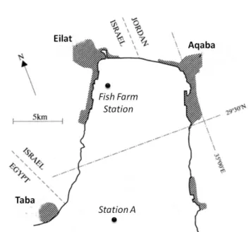
Water samples were collected at sampling Station A (29°28’N and 34°55’E) and the Fish Farm Station (29°32' N and 34°56' E) (Fig 3). The

Fish Farm Station point was near a Fish Farm that was operational until 17th

June 2008, the complete closure date of the Fish Farm, about halfway through the total sampling time. The maximum depth in the Fish Farm

Station point is 56 meters. The Station A sampling point is about 13 km

away from the Fish Farm Station, and has a 700 m maximum depth and no apparent direct anthropogenic influence.

To collect the parameter measurements and water samples a CTD-Rosette (Sea Bird) equipped with 11 Teflon-coated Niskin bottles (12 L), a CTD (SBE 19-02, SeaBird), Photometer, LICOR (LI-190SA) and a Fluorometer (Sea-Point Sensors Inc.) were used.

The dataset used for building the models contains measurements of: temperature (°C), salinity (ppt), oxygen (micromol/l), pH, alkalinity (meq/kg), NO3 (micromol/l), SiO4 (micromol/l), PO4 (micromol/l), and

chlorophyll a (microgr/l). Every measure was performed for both sampling stations. Irradiance data was also available every hour for the three years analyzed.

(15)

9

Fig. 3: Location of the sampling points “Fish Farm Station” and “Station A”

ANALYSIS OF TIME SERIES

At the beginning, the different time series were examined (nutrients,

chlorophyll a, temperature and irradiance), and bivariate correlations

between them were sought (chlorophyll a and temperature, chlorophyll a and each nutrient), with regression line and R2 (Microsoft Excel), Pearson’s

correlation coefficient (R) and p-value (MATLAB software). Statistical

analyzes were performed on the chlorophyll a time series to see if there were significant differences between the two sampling stations before and after the Fish Farm closure (t-test for dependent samples, STATISTICA software). Statistical analysis was also performed within each sampling station, to check if there were significant differences before and after the Fish Farm closure. The test was carried out for both the sampling stations for chlorophyll a, PO4, NO3 and SiOH4 (t-test for independent samples,

STATISTICA software). This step was crucial to understand how the data were linked to each other.

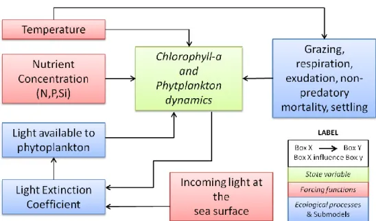
CONCEPTUAL DIAGRAM

A conceptual diagram was built containing the state variables, the forcing functions and how these components are interrelated (Fig. 4). In the present study chlorophyll a concentration and the phytoplankton sp. are the

(16)

10

state variables used to describe the state of the ecosystem. Forcing functions influence the state of the ecosystem. In this model the maximum growth rate of the state variable is limited by temperature, nutrient concentration and light available for the photosynthesis process. The other processes influencing algal dynamics (grazing, respiration, exudation, non-predatory mortality, and settling) are considered as functions of temperature.

Fig. 4: Conceptual model that show how forcing functions and ecological processes are interrelated for phytoplankton dynamics.

MATHEMATICAL FORMULATION OF THE PROCESS

The equation which describes the algal growth was chosen to model the dynamics of chlorophyll a (Jørgensen and Bendoricchio 2001):

(1)

represents the variation in the chlorophyll a (A) concentration per day. In

this differential equation A can either be the algal biomass or the

chlorophyll a concentration. represents the gross growth rate ; is the

respiration rate ; is the exudation rate ; is the non-predatory mortality rate ; is the settling rate and is the loss due to grazing

. In this model it was decided to lump parameters into a single loss parameter since this study is not aimed at discovering the cause of the loss in terms of chlorophyll a; moreover, quantifying the different

(17)

11

parameters would add unnecessary complexity to the model and require hitherto unavailable data. The parameter that represents the growth rate is usually modelled by the equation (Jørgensen and Bendoricchio 2001):

(2)

This equation was chosen because it represents a classic, general and simple method for modelling phytoplankton dynamics. In this equation is the maximum growth rate at the reference temperature . Whereas is a function of the factors limiting growth. The value of is achieved

under optimal, non–limiting conditions, with perfect availability of light and

nutrients. Functions represent the temperature

relationship, the light limitation andthe limitation of maximum growth rate due to nutrient starvation respectively.

Function limits the as a function of the water temperature. For this function two possible solutions were tried. It was possible to chose the usual Arrhenius exponential model (Jørgensen and Bendoricchio 2001):

₍₃₎

Where is the temperature data, is a parameter and its value should range between 1 and 1.05. The variation of this parameter increases the influence of temperature on the chlorophyll a time trajectory (e.g. it exacerbates peaks); was assumed to be 24°C.

The temperature can also be modelled with the skewed normal distribution around an optimum temperature (Jørgensen and Bendoricchio 2001):

₍₄₎

Where is the temperature data, if , if . is the minimum temperature under which the growth is zero, is the maximum temperature giving a non-zero growth, is the

optimum temperature for the growth.

Function that represents light limitation, in this case, is expressed as the measure of irradiance expressed in W/m². For this function two possible solutions were tried: the Michaelis-Menten equation, and the

(18)

12

Steel formulation. The Michaelis-Menten equation simulates a saturation

effect of light (Jørgensen and Bendoricchio 2001):

(5)

Where is the semisaturation constant and is the light intensity useful for photosynthesis, defined by the following equation (Jørgensen and Bendoricchio 2001):

₍₆₎

represents a coefficient that accounts for photosynthetic activity, namely , is the light intensity at the surface (W/m²), is the extinction coefficient in water body (0.035 m-1) and is the water depth (m) (Hill 1963, Jørgensen and Bendoricchio 2001).

The second light limitation model is an optimum curve, or Steel formulation (Jørgensen and Bendoricchio 2001):

(7)

Where is the light intensity usabal for photosynthesis, is the optimum light intensity for photosynthesis, this value can be modified according to the acclimation of phytoplankton to light variation at depth and time.

Function represents the limitation by nutrient availability. For this function the Michaelis-Menten kinetics or Monod approach was chosen, where the is limited by the external concentration of the nutrient

(Jørgensen and Bendoricchio 2001):

(8)

represents the external concentration of nutrient expressed in micromol/l, represents the semi-saturation constant. The semi-saturation constant is the nutrient concentration at which the reaction rate is at its half-maximum. It is a measure of the algal affinity for nutrients, which is linked to phytoplankton growth and, thus, to chlorophyll a production. A low value of and an high value of indicate high and low affinities respectively. If there was inserted more than one nutrient in the model, several possibilities of interaction were tested using multiplication, arithmetic

(19)

13

mean, harmonic mean and minimum of Liebig (Jørgensen and Bendoricchio

2001).

Several models were tried for testing and comparing different forecast scenarios and understanding which forces determine phytoplankton dynamics. The models were made with different combinations of nutrients:

- without any nutrient (only temperature); - with PO4 only;

- with NO3 only;

- with SiOH4 only;

- with PO4 and SiO4;

- with NO3 and PO4;

- with NO3, PO4 and SiO4;

- with different nutrients until and after the closure of the Fish Farm; with different time scales to understand if it is better to use a model that considers or ignores the Fish farm closure:

- three years;

- prior and following the Fish Farm closure;

and with different constants to understand if the Fish Farm Station closure produced a significant change in phytoplankton community composition or not (it is assumed that different constants correspond to different phytoplankton species):

- remains the same over three years of simulation; - changes after the Fish Farm closure.

TRANSFER TO COMPUTER

To build the model, the MATLAB software was used (version 7.6.0.324 R2008a), in particular a tool named Simulink. Simulink is an environment for multidomain simulation and Model-Based Design for dynamic and embedded systems.

VERIFICATION

Verification of the model was performed. It is a subjective assessment of the behaviour of the model, to test its internal logic. The

(20)

14

values of the parameters were changed, one by one, to see if the model reacted as expected and if it was stable in the long term (Jørgensen and Bendoricchio 2001).

SENSITIVITY ANALYSIS

Sensitivity analysis was carried out by changing the parameters, forcing functions, initial values and submodels, and observing the corresponding response in the state variable. This is a fundamental step to learn the proprieties of the model, since through this analysis it is possible to get a good overview of the most sensitive components and processes in the model. The sensitivity of any one parameter was defined by the following equation (Jørgensen and Bendoricchio 2001):

(9)

Where is the sensitivity, is a parameter, and is the state variable (chlorophyll a). The values of parameters were changed, one by one, by +2% and -2%. It was chosen to change the parameters by +2% and -2% because the models were extremely sensitive to larger changes of some of the parameters.

CALIBRATION

Calibration is an attempt to find the best agreement between computed and observed data by varying some selected parameters. The aim of calibration is to improve data fit through parameter estimation. In this model the parameters found in the literature, which referred to ecosystems similar to that of the Gulf of Aqaba, were considered just as approximate, starting values. Initially, in this model, calibration was performed manually, followed by an automatic calibration using Simulink (MATLAB). The automatic calibration provides a graphical user interface for estimating the parameters and initial states of the model using empirical input and output data pairs.

(21)

15 VALIDATION

Validation consisted of testing the selected parameters for the Fish

Farm Station with an independent set of data, in this specific case referring

to the sampling Station A in the northern Gulf of Aqaba. This operation is useful for testing if the model is replicable or if the model is valid only for the Fish Farm Station. After validation the differences between the various

Fish Farm Station and Station A models was assessed.

CONFRONTING MODELS

Different models were compared by three indexes: Residual Sum of Squares (RSS), Nash–Sutcliffe Model Efficiency Coefficient (E) and Akaike Information Criterion (AIC) (Akaike 1974, Moriasi et al. 2007, Nash and Sutcliffe 1970).

Residual Sum of Squares (RSS) is a measure of the discrepancy between the data and the estimation of the model. The index is the sum of squares of residuals. The residuals are the difference between the sample and the estimated data:

(10) Where is modelled data at time , is observed data of chlorophyll a at time . The closer the RSS value is to 0 the more accurate the model is. The Nash–Sutcliffe Model Efficiency Coefficient (E) was used to assess the predictive power of the models:

(11)

Where is modelled data at time , is observed data of chlorophyll a at time , is the average of observed data (Moriasi et al. 2007, Nash and Sutcliffe 1970). This index can range from , if there is a perfect match between modelled data to the observed data. If the model predictions are as accurate as the mean of the observed data. If the residual variance (described by the numerator) is larger than the data variance (described by the denominator), the closer E is to 1 the more accurate the model is. Since all models were applied to the same dataset of

(22)

16

observed chlorophyll a data, the denominator of E was constant and, thus, the use of E was perfectly equivalent to using RSS, as can be appreciated by comparing equations (10) and (11).

The Akaike Information Criterion (AIC) measures the relative goodness of fit (Akaike 1974). This index includes a penalty that is an increasing function of the number of estimated parameters; this measure is particularly important because equations (10) and (11) do not take into account the number of parameters (Akaike 1974):

(12)

Where is the number of parameters and is the Chi-squared distribution:

(13)

Where is the number of sampled points, is modelled data at time , is observed data of chlorophyll a at the time . The more negative the AIC index value is, the more accurate the model is. If the difference in the AIC value, between two models, is less than two they are roughly equivalent (Akaike 1974).

(23)

17

RESULTS

ANALYSIS OF TIME SERIES

At the beginning it was necessary to analyze and understand the time series of the principal factors that control the ecosystem in question. The time series of the principal factors that can drive phytoplankton dynamics are shown in Fig. 5, Fig. 6, Fig. 7, Fig. 9, Fig. 10 and Fig 11.

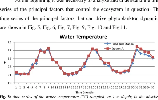
Fig. 5:time series of the water temperature (°C) sampled at 1-m depth; in the abscissa “time 1” corresponding to the first month of sampling (14th January 2007) and “time 35” the last month (28th December 2009).

In the time series of the water temperature there were no evident differences between the Fish Farm Station data and Station A data. In both sampling stations the seasonality of this forcing function can be seen: high temperature in the summer-fall months and low temperature in the winter-spring months.

Fig. 6: time series of the irradiance (W/m2_{) sampled every day from 14}th_{January 2007 to}

28th December 2009 in the Interuniversity Institute for Marine Science (IUI), Eilat.

In this graph the sunlight irradiance (W/m2) was represented, these data were used for both the sampling stations. The same seasonal trend can be seen, similar to the pattern of the water temperature (Fig. 5).

0 50 100 150 200 250 300 350 400 0 200 400 600 800 1000 W /m 2 Time (day)

Irradiance

19 21 23 25 27 29 1 2 3 4 5 6 7 8 9 10 11 12 13 14 15 16 17 18 19 20 21 22 23 24 25 26 27 28 29 30 31 32 33 34 35 °C Time (month)

Water Temperature

Fish Farm Station Station A

(24)

18

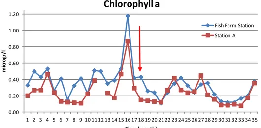
Fig. 7: time series of the chlorophyll a concentration (microgr/l) sampling from 14th

January 2007 in both the sampling stations.

Figure 7 shows the time series of chlorophyll a concentration measurements. The red arrow, in this graph and in all the following graphs, indicates the 17th June 2008, the date of the complete closure of the Fish Farm. It is possible to see how before the closure of the Fish Farm the concentration of chlorophyll a in the Fish Farm Station was significantly different from its concentration in Station A (t-test for dependent samples:

t=6.57; p<0.0001). From the point indicated by the red arrow to the end of

the time series, the chlorophyll a data of Station A and Fish Farm Station appear to become more similar (t-test for dependent samples: t=1.95;

p=0.069854).

Fig. 8: The two graphs show the time series of chlorophyll a with the regression line (indicating the trend over time) and R2, for both sampling stations. The red line indicates the Fish Farm closure.

In Fig. 8 the outlier in chlorophyll a data was deleted for month 16, because it excessively influenced the regression line. The same procedure was

0.00 0.20 0.40 0.60 0.80 1.00 1.20 1 2 3 4 5 6 7 8 9 10 11 12 13 14 15 16 17 18 19 20 21 22 23 24 25 26 27 28 29 30 31 32 33 34 35 m ic rog r/ l Time (month)

Chlorophyll a

(25)

19

applied to the graphs below that include a regression line (Fig. 12, Fig 13, Fig. 14 and Fig. 15). The first graph of Fig. 8 shows how, in the Fish Farm

Station, the chlorophyll a trend decreases over time (Pearson’s correlation coefficient (R) R=-0.51, p=0.0019), in particular the concentration

decreased after the Fish Farm closure. Indeed there is a significant difference in chlorophyll a before and after the Fish Farm closure (t-test for independent samples: t=3.13; p=0.007). In the Station A graph there is a small decrease in chlorophyll a over time (R=-0.09, p=0.5962) but it is not as strong as in the Fish Farm Station and there are no significant differences (t-test for independent samples: t=0.97; p=0.075).

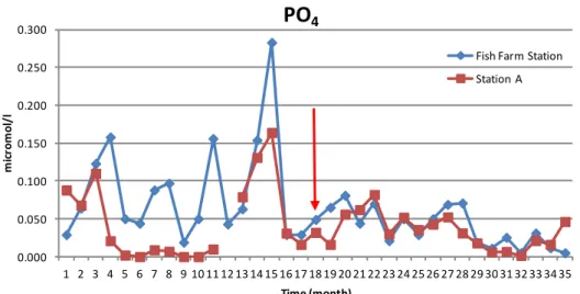
Fig. 9: Time series of PO4 concentration (micromol/l) from 14th January 2007 at both

sampling stations.

It is evident that before the Fish Farm closure , the concentration of PO4 was

higher in the Fish Farm Station than it was in Station A. After the Fish Farm closure the trend and concentrations of PO4 became more similar in both

sampling stations. The statistical analysis of the Fish Farm Station data reveals that there are significant differences before and after the Fish Farm closure (t-test for independent samples: t=2.67; p=0.000564). In the Station

A data there are significant differences before and after the red arrow (t-test

for independent samples: t=0.53; p=0.002352).

0.000 0.050 0.100 0.150 0.200 0.250 0.300 1 2 3 4 5 6 7 8 9 10 11 12 13 14 15 16 17 18 19 20 21 22 23 24 25 26 27 28 29 30 31 32 33 34 35 m ic rom ol /l Time (month)

PO

₄

(26)

20

Fig. 10:Time series of the NO3 concentrations (micromol/l) from 14th January 2007 in both

Both nitrate concentrations and peaks thereof at both stations were higher before the closure of the farm than during the following period. For both station data-sets the statistical analysis shows a significant difference before and after the red arrow (t-test for independent samples Fish Farm Station:

t=2.70; p<0.0001 and Station A: t=2.59; p<0.0001). Also, the time series

show that concentrations next to the Fish Farm were higher than in the open sea, a difference that disappeared later on.

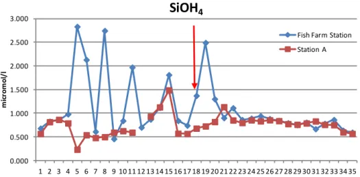
Fig. 11: time series of the SiOH4 (micromol/l) sampling from 14th January 2007 in both

In the silicate graph the pattern of SiOH4 is very different at the two

sampling stations: before the red arrow in the Fish Farm Station data there are a short, strong fluctuations compared to Station A data. About three months after the Fish Farm closure such fluctuations were no longer

0.000 0.500 1.000 1.500 2.000 2.500 3.000 3.500 1 2 3 4 5 6 7 8 9 10 11 12 13 14 15 16 17 18 19 20 21 22 23 24 25 26 27 28 29 30 31 32 33 34 35 m ic rom ol /l Time (month)

NO

3

Fish Farm Station Station A 0.000 0.500 1.000 1.500 2.000 2.500 3.000 1 2 3 4 5 6 7 8 9 10 11 12 13 14 15 16 17 18 19 20 21 22 23 24 25 26 27 28 29 30 31 32 33 34 35 m ic rom ol /l Time (month)

SiOH

₄

(27)

21

observed, and the trend of SiOH4 became similar in the two sampling

stations (in the Fish Farm Station the concentration average is higher before the Fish Farm closure, in Station A it is higher after the closure). In both datasets there were significant differences before and after the Fish Farm closure (t-test for independent samples Fish Farm Station: t=2.33;

p<0.0001 and Station A: t=-1.23; p=0.001605).

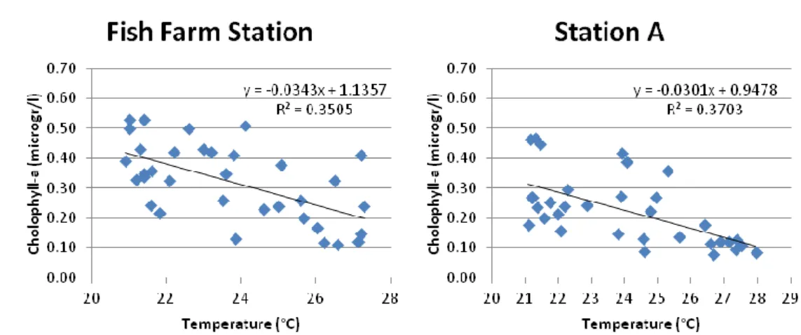
Fig. 12: Time series of chlorophyll a concentration (micromol/l)as function of the water temperature (°C), both data sets were collected from 14th January 2007.

In these two graphs the chlorophyll a data is shown as a function of temperature that was measured in the Fish Farm Station and Station A. Both graphs show how the chlorophyll a concentration decreases with increasing temperature (Pearson’s correlation coefficient (R) is similar in the Fish

Farm Station R=-0.59, p=0.00022684 and Station A R=-0.61, p=0.00012417). In both chlorophyll a datasets an outlier datum in the 16th

month was deleted (1.18 microgr/l in the Fish Farm Station and 0.87 microgr/l in the Station A). The same procedure was applied to the following graphs.

(28)

22

Fig. 13: Time series of chlorophyll a concentration (microgr/l) as function of PO4

concentration (micromol/l). Both data sets were collected from 14th January 2007.

These two graphs show the sampled chlorophyll a data as function of the PO4 data: an increase in PO4 concentration entails an increase in the

phytoplankton population and, as a consequence, an increase in detected

chlorophyll a. In both stations there is a positive correlation, which is

stronger in the Fish Farm Station (R=0.51, p=0.0019) than in Station A (R=0.38, p=0.0271).

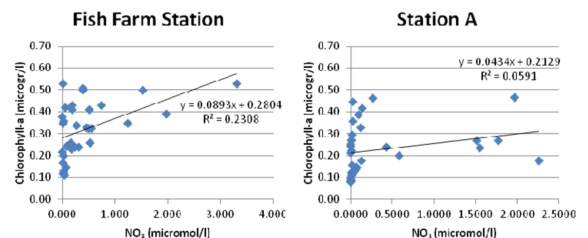
Fig. 14: Time series of chlorophyll a (microgr/l) as a function of NO3 concentratioon

(micromol/l., Both data sets were collected from 14th January 2007.

The first graph shows the correlation between the field measure of

chlorophyll a and NO3 in the Fish Farm Station (R=0.46, p=0.0064). The

second graph shows the same correlation, but concerning the data collected in Station A (R=0.24, p=0.1655). A negative correlation can be seen in both sampling stations, which is more marked in the Fish Farm Station.

(29)

23

Fig. 15:Time series of the chlorophyll a concentration (microgr/l) as a function of SiOH4

(micromol/l). both data sets collected from 14th January 2007.

These two graphs show the correlation between SiOH4 and chlorophyll a

(Fish Farm Station R=0.15, p=0.4034; Station A R=0.23, p=0.1860).

SIMULATION OF THE FISH FARM STATION MODELS

Verification (p. 12) showed how the variation of parameters implied a change in the chlorophyll a simulation.

Increasing the constant:

- " " (2), chlorophyll a simulated concentration increases over

time

- " " (1), chlorophyll a simulated concentration decreases over time - " " (2), chlorophyll a simulated concentration increases over time

- " " (5),chlorophyll a simulated concentration decreases over time

- " " (8), chlorophyll a simulated concentration decreases over time - " " (3), increases in the maximum value of chlorophyll a

concentrations, simultaneously decreases in the minimum value of

chlorophyll a concentrations.

Decreasing the constant:

- " " (2), chlorophyll a simulated concentration decreases over

time;

- " " (1), chlorophyll a simulated concentration increases over time; - " " (2), chlorophyll a simulated concentration decreases over

time;

- " " (5), chlorophyll a simulated concentration increases over time; - " " (8), chlorophyll a simulated concentration increases over time;

(30)

24

- " " (3), decreases in the maximum value of chlorophyll a concentrations, simultaneously increases in the minimum value of

chlorophyll a concentrations.

Changing the constant:

- " " (4), chlorophyll a simulated concentration greatly increases in

correspondence to the value;

- " " (7), chlorophyll a simulated concentration greatly increases in

correspondence to the value.

The sensitivity analysis (p. 12) shows that the parameters that most strongly influence the chlorophyll a simulated values are and

. This finding means that the preview constants compared to the others are more sensitive to small variations. Hence, small changes in one or more of these four constants cause great changes in the chlorophyll a simulated trend.

All the following tables show some models with the number of parameters, the results of Residual Sum of Squares (RSS), the Nash– Sutcliffe Model Efficiency Coefficient (E) and the Akaike Information Criterion (AIC). Abbreviations represent the processes found in the model. In all the abbreviations of the models the forcing functions of grazing, respiration, exudation, non-predatory mortality and settling were omitted because these parameters were included in all the models. Station A

chlorophyll a time series (Fig. 7) shows how the chlorophyll a values stay

low during the summer months and increase during the winter months, as described in the typical Gulf of Aqaba phytoplankton dynamics (Al-Najjar et al. 2007, Mackey et al. 2007, Mackey et al. 2009). Conversely, in the

chlorophyll a Fish Farm Station time series (Fig. 7) low chlorophyll a

concentrations cannot be seen in the summer months but concentrations are high in winter, thus the typical phytoplankton seasonality dynamic is lessened, presumably by the nutrient input from the fish exreta and decomposing food residues before the Fish Farm closure. For this reason it was chosen to not apply a seasonal pattern to the Fish Farm Station simulation models.

(31)

25

Table 1 summarizes the results for 8 simple models for the Fish Farm Station. In these models the additional forcing functions are

temperature (with optimum (4) or Arrhenius (3) function) and only one nutrient (with Michaelis-Menten (8) function) selected from NO3, PO4 and

SiOH4. Abbreviations indicate which parameters are inserted in the model:

Table 1

T°(OPT): a model with only temperature to regulate the dynamics of

chlorophyll a; ―OPT‖ indicates that the function selected for the model was

the optimum function.

T°(EXP): a model with only temperature to regulate the dynamics of

chlorophyll a; ―EXP‖ indicates that the function selected for the model was

the Arrhenius function.

In the other models of Table 1, after the temperature function, there is the nutrient that regulates the simulated dynamics of chlorophyll a (NO3, PO4 or

SiOH4).

In all models it can be seen how the Arrhenius relation for the temperature function is much better than the optimum formulation. For that reason in the following model, the exponential relation for the temperature function (Arrhenius) was applied.

The following graph shows the time series simulations of model T°(EXP) and the models that result in the best simulations (Table 1): T°(EXP)_NO3 and

T°(EXP)_PO4. In this and all following graphs, the blue line represents the simulated data and the blue dots represent the real sampled data.

N°Parameters RSS E AIC T°(OPT) 8 4.21 -2.366 -58.123 T°(EXP) 6 1.333 -0.066 -102.381 T°(OPT)_NO3 9 2.129 -0.703 -79.981 T°(EXP)_NO3 7 1.024 0.181 -109.614 T°(OPT)_PO4 9 1.787 -0.429 -86.117 T°(EXP)_PO4 7 1.084 0.133 -107.614 T°(OPT)_SiOH4 9 2.333 -0.866 -76.782 T°(EXP)_SiOH4 7 1.299 -0.038 -101.286

(32)

26

Simulation Graph 1

The Simulation Graph 1 shows how the dynamics of chlorophyll a is similar over the three years. This is because, in this model, the dynamics of

chlorophyll a is modelled by only the temperature forcing function and this

function follows the seasonal water temperature data (Fig. 5).

(33)

27

Simulation Graph 2 and Simulation Graph 3 show the simulation with the

addition of NO3 or PO4. The results of simulations improve in both

conditions and the trend changes year by year, which is due to the interaction between the temperature forcing function and the nutrient forcing function.

Table 2 shows some models with various combinations of nutrients.

The function of temperature with the Arrhenius function is inserted in all these models (indicated with T°).

Table 2

T°_PO4_X_NO3: the Michaelis-Menten function for PO4 and NO3 was inserted

in this model. The values of the Michaelis-Menten function for the nutrients

N°Parameters RSS E AIC T°_PO4_X_NO3 8 0.998 0.202 -108.519

T°_PO4_NO3_SiOH4_liebig 9 1.759 -0.406 -86.672

T°_PO4_NO3_liebig 8 1.645 -0.315 -91.027

T°_NO3_kvar 8 0.883 0.294 -112.776

T°_PO4_kvar 8 1.077 0.139 -105.836

T°_NO3_BFC_PO4_PFC 8 0.842 0.327 -114.477

T°_PO4_BFC_NO3_PFC 8 1.262 -0.009 -100.294

T°_NO3_X_SiOH4_BFC_PO4_PFC 9 1.318 -0.054 -96.772

(34)

28

are multiplied at every time step of the model (the multiplication in the

Table 2 is indicated by ―X‖): (14)

The function applied in this model is a variation of equation (8), where PO4

indicates the PO4 data at time t, NO3 indicates the NO3 data at time t, the

semi-saturation constant for PO4 and the semi-saturation constant for

NO3.

T°_PO4_NO3_SiOH4_liebig: the minimum of the Liebig Law to define the limiting nutrient for each simulation time of the model was inserted: the model chose the lowest value of the results of three functions (8), one for each nutrient.

T°_PO4_NO3_liebig: this model is the same as the previous one but without SiOH4 data.

T°_NO3_kvar and T°_PO4_kvar: these two models have one nutrient each (NO3

or PO4) to regulate the phytoplankton dynamics. The ( ) in the function (8)

is the only parameter that can change after the Fish Farm Station closure. This is the first model where an ecological change due to the Fish Farm closure was simulated.

T°_NO3_BFC_PO4_PFC and T°_PO4_BFC_NO3_PFC: in the first model NO3 limits

the phytoplankton growth rate before the Fish Farm closure and PO4 limits

the growth rate after the Fish Farm closure. In the second model there is the opposite situation: PO4 limits the growth rate before and NO3 limits the

phytoplankton growth rate after the Fish Farm closure. These models and the two models below were made to understand if the Fish Farm activity might have caused a change in the phytoplankton dynamics, resulting from the nutrients that regulate it. Therefore, a nutrient or nutrients were added before the Fish Farm closure and a different condition was found after the Fish Farm closure.

T°_NO3_X_SiOH4_BFC_PO4_PFC: here NO3 and SiOH4 limits the growth before

the Fish Farm closure, the values for the nutrients function are multiplied at each time. After the Fish Farm closure PO4 begins to limit the

(35)

29

T°_NO3_BFC_SiOH4_PFC: in this model NO3 limits the growth rate before the

Fish Farm closure and SiOH4 limits the phytoplankton growth after the Fish

Farm closure.

The following graph shows the time series simulations of the models that have the best results (Table 2) from the index (RSS, E and AIC):

T°_PO4_X_NO3, T°_NO3_kvar, T°_PO4_kvar, T°_NO3_BFC_PO4_PFC and

T°_NO3_BFC_SiOH4_PFC.

Simulation Graph 4 shows the interaction between two nutrients, PO4 and

NO3. In this Simulation Graph there is no influence by the Fish Farm

closure.

(36)

30

Simulation Graph 5 and Simulation Graph 6 are the first simulations that

include the semi-saturation constant ( ) variation of the Michaelis-Menten function for the nutrient after the Fish Farm closure. In those and the following Simulation Graph the time when there is a change in is represented by the red line.

Simulation Graph 7 simulates a variation of the nutrients that regulate the

phytoplankton dynamics: before the Fish Farm closure NO3 is limiting and

(37)

31

Simulation Graph 8 simulates a variation of the nutrients that regulate the

phytoplankton dynamics: before the red line NO3 is limiting and after SiOH4

is limiting.

Table 3 shows models with the addition of the light limiting function

(5) and (7):

Table 3

Table 3 shows how the addition of the light function improves the models;

this is evident in the AIC value, which also takes into account the increase in the number of parameters (see Table 1 and Table 2). The table also highlights how the Michaelis-Menten function (saturation) for light is better than the Steel formulation (optimum). Table 3 also includes the best model obtained for the Fish Farm Station data:

T°_NO3_BFC_PO4_PFC_LIGHT_SATURATION, in this simulation it was assumed that nitrogen regulates the phytoplankton dynamics before the Fish Farm

N°Parameters RSS E AIC

T°_LIGHT_SATURATION 7 1.308 -0.046 -101.036

T°_LIGHT_OPTIMUM 7 4.034 -2.225 -61.624

T°_NO3_kvar_LIGHT_SATURATION 9 0.706 0.435 -118.62

T°_NO3_kvar_LIGHT_OPTIMUM 9 3.555 -1.842 -62.046

T°_NO3_BFC_PO4_PFC_LIGHT_ SATURATION 9 0.693 0.446 -119.29

T°_NO3_BFC_PO4_PFC_LIGHT_OPTIMUM 9 1.446 -0.156 -93.537

T°_NO3_BFC_SiOH4_PFC_LIGHT_ SATURATION 9 0.725 0.42 -117.698

(38)

32

closure and that phosphate regulates the phytoplankton dynamics after the Fish Farm closure.

The following graphs show simulations of the models reported in

Table 3. The following simulation displays differences between the

saturation function (Michaelis-Menteen) and the optimum function (Steel

Formulation).

Simulation Graph 9 and Simulation Graph 10 give different results with

(39)

33

the Fish Farm closure. The light function is the only difference between the two models (saturation and optimum).

Simulation Graph 11 and Simulation Graph 12 show two simulations of the

model that includes NO3 as limiting nutrient before the Fish Farm closure

and SiOH4 as limiting nutrient after the Fish Farm closure. The only

difference between these graphs is again the light function.

Table 4 shows models with different combinations of nutrients for

(40)

34

indicates that the best model is T°_NO3_BFC_PO4_PFC_LIGHT_SATURATION (Table 3):

Table 4

T°_NO3_BFC_PO3_X_NO3_PFC_LIGHT: in this model, before the Fish Farm closure NO3 was inserted as limiting nutrient and after closure PO4 and NO3

were added as limiting nutrients; the value for the nutrients function were multiplied at each time.

T°_NO3_BFC_PO4_X_SiOH4_PFC_LIGHT: in this model, before the Fish Farm closure NO3 was inserted as a limiting nutrient followed by PO4 and SiOH4;

the value for the nutrient function were multiplied at each time.

In the other model in Table 4 ―liebig‖ indicates that the nutrient was chosen by the minimum of Liebig, ―arithmean‖ indicates that there is an arithmetic mean between the two nutrients:

(15)

is a variation of the equation (8); in this function is the

concentration of the first nutrient, is the concentration of the second nutrient, is the semi-saturation constant of the first nutrient and is the semi-saturation constant of the second nutrient. ―Harmonmean‖ indicates that there is a harmonic mean between both nutrients:

(16)

is a variation of the equation (8), where and are the

concentration of the first and second nutrient, and are the semi-saturation constant of the first nutrient and the second nutrient.

T°_NO3_BFC_PO3_X_NO3_PFC_LIGHT 10 0.774 0.381 -113.392

T°_NO3_BFC_PO4_NO3_liebig_PFC_LIGHT 10 0.695 0.445 -117.183

T°_NO3_BFC_PO4_NO3_arithmean_PFC_LIGHT 10 0.761 0.392 -114.002

T°_NO3_BFC_PO4_NO3_harmonmean_PFC_LIGHT 10 0.763 0.39 -113.911

T°_NO3_BFC_PO4_X_SiOH4_PFC_LIGHT 10 0.717 0.426 -116.064

T°_NO3_BFC_PO4_SiOH4_liebig_PFC_LIGHT 10 0.73 0.416 -115.43

T°_NO3_BFC_PO4_SiOH4_arithmean_PFC_LIGHT 10 0.716 0.427 -116.065

(41)

35 BEST FISH FARM STATION MODELS

Table 5

Table 5 shows the best Fish Farm Station models, based on the results of

the RSS, E and AIC indexes. The index results are similar, the best result was achieved by model T°_NO3_BFC_PO4_PFC_LIGHT_ SATURATION. Before the Fish Farm closure the conditions that regulated the chlorophyll a dynamics were the same in all the models in Table 5: temperature function (3), the nutrient that regulates the phytoplankton dynamics before the Fish Farm closure NO3 with equation (8) and the light function with equation (5).

All the models in Table 5 include a change in the nutrient/s that regulate the phytoplankton dynamics after the Fish Farm closure: either in the constant, or in the nutrient/s or both.

In conclusion, in all models the conditions before the Fish Farm closure are the same, the models differ only for the nutrients function (8) that changes after the Fish Farm closure.

FISH FARM MODEL VALIDATION

The validation consists of testing the best model of the Fish Farm

Station with an independent set of data, in this specific case the Station A

dataset. Table 6 shows the result of validation of the best Fish Farm Station models (Table 5). For every four models in Table 6 the index values resulting from the simulation after the calibration of the same models are also shown.

T°_NO3_kvar_LIGHT_SATURATION 9 0.706 0.435 -118.62

T°_NO3_BFC_PO4_PFC_LIGHT_ SATURATION 9 0.693 0.446 -119.29

T°_NO3_BFC_SiOH4_PFC_LIGHT_ SATURATION 9 0.725 0.42 -117.698

(42)

36

Table 6

In all the examples the index value for the validation is poor; this is evident from the results of RSS, E and AIC indices. The same models with the calibration also gives poor index results.

The table below shows only the simulation of two models of Table 6 (one validation and one calibration); this is because all simulations are not good and similar. Therefore is not useful to see all the simulations of the model reported in Table 6.

Simulation Graph 13 shows the validation of model

T°_NO3_BFC_PO4_PFC_LIGHT_SATURATION: the Station A dataset was inserted in the Fish Farm Station model. The results of index (RSS, E and AIC) are

CALIBRATION

T°_NO3_BFC_PO4_PFC_LIGHT_ SATURATION

9 2.359 -1.827 -76.397

CALIBRATION

T°_NO3_BFC_PO4_NO3_liebig_PFC_LIGHT_SATURATION

10 2.264 -1.712 -75.839

VALIDATION

T°_NO3_BFC_PO4_PFC_LIGHT_ SATURATION

9 2.658 -2.184 -72.228

CALIBRATION

T°_NO3_BFC_SiOH4_PFC_LIGHT_ SATURATION

9 2.278 -1.73 -77.61

VALIDATION

T°_NO3_BFC_PO4_NO3_liebig_PFC_LIGHT_SATURATION

10 2.559 -2.066 -71.547

CALIBRATION

T°_NO3_kvar_LIGHT_SATURATION

9 2.158 -1.586 -79.511

VALIDATION

T°_NO3_BFC_SiOH4_PFC_LIGHT_ SATURATION

9 2.549 -2.054 -73.685 VALIDATION T°_NO3_kvar_LIGHT_SATURATION -73.617 -2.06 2.554 9

(43)

37

not good and the simulation data do not reflect the real pattern of

chlorophyll a.

Simulation Graph 14 shows the preview model but with the calibration of

all the parameters, this is the best result achieved.

SIMULATION OF STATION A MODELS

Table 7

To obtain a good simulation for Station A models that include a simplification for the seasonality of phytoplankton dynamics were made, in addition to the temperature function (3) and the light function (5). In all the models reported in Table 7 it was decided that in winter and spring each year the nutrient to regulate chlorophyll a dynamics should be NO3, which

regulates the dynamics of Cryptophyta and Chlorophyta (more abundant in this season), whereas in summer and fall it should be PO4 which regulates Prochlorococcus and Synechococcus dynamics, which are more abundant in

this season (Al-Najjar et al. 2007, Mackey et al. 2007, Mackey et al. 2009). The previously explained seasonality of phytoplankton was not recreated directly by the model because it would double the number of parameters.

T°_NO3_PO4_SEASON_LIGHT_SATURATION 9 0.798 0.043 -114.314

T°_NO3_PO4_SEASON_LIGHT_SEASON_SATURATION 10 0.793 0.050 -112.575

T°_NO3_PO4_SEASON_LIGHT_SATURATION_kvar 11 0.329 0.606 -141.390

(44)

38

This would lead to a much too complex model (with many parameters), especially considering the few real chlorophyll a measurements. Therefore, the phytoplankton seasonality pattern was "forced" by making change because there is a real change in the species that represented most of the

chlorophyll a. In the Gulf of Aqaba, during Prochlorococcus and Synechococcus growth, some studies show that this Cyanobacteria have

higher phosphorus than nitrogen requirements (Fuller et al. 2005, Mackey et al. 2009). The abbreviation ―kvar‖ indicates that can change after the

Fish Farm Station closure.

The second and last models of Table 7 show how if the simulation takes into account seasonality for the light function (with a change of the light function, as for the nutrients) E improves slightly with respect to the models without seasonality for the light function, but AIC worsens.

Simulation Graph 15 shows how after the Fish Farm closure the simulation

(45)

39

If the model includes the possibility for to change after the Fish Farm closure, the model simulation and the index value improve, in particular after the red line (see Simulation Graph 15).

Models containing seasonality, with or without being able to change after the Fish Farm closure, were applied to the Fish Farm Station dataset. Table 8 shows the index values:

Table 8

In both models calibration was performed, but as seen by the index values, the element that controls the Fish Farm Station phytoplankton dynamics is the Fish Farm activity (Table 5) and not the seasonality (Table 8).

T°_NO3_PO4_SEASON_LIGHT_SATURATION 9 3.886498 -2.1074 -58.9244

(46)

40

DISCUSSION

TIME SERIES

All the graphs of the time series after the Fish Farm closure, in particular the one about the Fish Farm Station data, show a decrease in the principal nutrients: NO3, PO4 and SiOH4 (Fig. 9, Fig. 10 and Fig. 11). Thus, from 17th

June 2008 onwards, when the Fish Farm closed, there is a lower concentration of nutrients. The Fish Farm Station nutrient concentration data are higher than those of Station A, but only before 17th June 2008, which was the date of the Fish Farm closure (Fig. 9, Fig. 10 and Fig. 11). This is the first statistically significant proof of the impact of the Fish Farm activities on at least the northernmost part of the Gulf, also hinting at a lesser effect on the entire Gulf as seen from the changes in nutrient concentrations at Station A before and after closure of the farming activity.

The graph of chlorophyll a reveals marked differences between Fish

Farm Station data and Station A data. In particular, the chlorophyll a

concentration is higher in the Fish Farm Station than it is in Station A; this is because there is a corresponding high nutrient concentration caused by the Fish Farm activity. This mean difference was greater (and statistically significant) before the fish farm closure (Huang et al. 2011). In both sampling stations the chlorophyll a concentration decreases over the sampling time (Fig. 8). In particular, lower chlorophyll a concentrations in both sampling stations are evident after the Fish Farm closure. This is more evident in the Fish Farm Station data (Fig. 8), but there is also a (weaker) decrease in Station A data. This might mean that the Fish Farm activity influences the concentration of nutrients which in turn influences the phytoplankton dynamics. This happens in both stations, but more markedly in the Fish Farm Station due to its proximity to the Fish Farm and its nutrient emissions. The model clearly underscores the validity of

chlorophyll a and of phytoplankton as signal amplifiers for eutrophication

processes and as such early warning management tools for marine conservation and management.

(47)

41

It is interesting to see how in Station A there are similar chlorophyll

a concentration patterns during summer and winter months (in all the

sampling years) (Fig. 7). This can be linked to the typical seasonal dynamics of phytoplankton in the gulf: when the nutrients and chlorophyll a concentration is high, in winter, eukaryotic algae in particular cryptophyta and chlorophyta dominate the phytoplankton community (Al-Najjar et al. 2007, Mackey et al. 2007, Mackey et al. 2009). When the nutrients and

chlorophyll a concentration is low, in summer and fall, picophytoplankton,

in particular Prochlorococcus and Synechococcus are more abundant with respect to other phytoplankton species (Al-Najjar et al. 2007, Mackey et al. 2007, Mackey et al. 2009). The same interpretation is not true for the Fish

Farm Station, in particular before the Fish Farm closure (Fig. 7). The

difference in the response of phytoplankton near the farms to seasonal nutrient inputs due to mixing from that of the open water pelagic domain is a text book example. It tells apart the exquisite sensitivity of oligotrophic phytoplankton assemblages, exemplified by Station A, to even minor eutrophication, from the insensitivity of nutrient replete ones to increase in nutrient availability.

The negative correlation of water temperature and chlorophyll a means that in the summer month, with an high value of irradiance, there are low chlorophyll a concentration while in winter, with a low value of irradiance, an high concentration of chlorophyll a (Fig. 6, Fig.8), that corresponds to the general phytoplankton dynamics in the Gulf of Aqaba (Al-Najjar et al. 2007, Mackey et al. 2007, Mackey et al. 2009). The lack of the typical pattern (high chlorophyll a concentration in winter months and low concentration in summer months) in the chlorophyll a time series probably indicates that there is a different process than temperature/light (that have a cyclical pattern: high value in summer months and low in winter) that regulates the phytoplankton dynamics, probably the nutrients. This is evident in the Fish Farm Station data, in particular in the summer and fall months, before the Fish Farm closure where is not possible to see the typical seasonality, instead the seasonality becomes more visible after

(48)

42

the Fish Farm closure and in all the three year Station A chlorophyll a data (Fig. 7).

In the graphs of NO3 (Fig. 10) it is possible to see the peak in

correspondence of the 15th month (middle of march 2008), which was probably due to an event of upwelling caused by very intense deep mixing (Iluz et al. 2009). There is also the same situation for the PO4 data, and the

result of this nutrients increase is a strong spring bloom (Gordon et al. 1994, Genin et al. 1995). This is evident in the chlorophyll a time series for both the sampling stations: following high levels of this two nutrients there is an increase of the chlorophyll a concentration on months 15 and 16 (thus, a slightly time shifted effect), because PO4 (in particular) and NO3 are the

main two nutrients limiting the phytoplankton growth rates in the Gulf of Aqaba (Suggett et al. 2009). From the correlations between chlorophyll a and these two nutrients it is evident how high concentrations of nutrients lead to corresponding high chlorophyll a concentrations, which is to be expected in a oligotrophic system such as the Gulf of Aqaba, especially underscored in the summer.

It is interesting to examine the dynamics of the SiOH4: before the

Fish Farm closure there is a particular time trajectory, with a fluctuating concentration of SiOH4. After two months of the Fish Farm closure the

trend became constant and very similar in both sampling stations. It is plausible that the diatoms, that are characterized by a unique cell wall made of silica, are implicated in this pattern, but since there are not cell count data available, it is not possible to confirm this hypothesis.

FISH FARM STATION MODELS

In the Table 1 is evident how in all the models the Arrhenius exponential function is better than the Optimum function (RSS, E and AIC indices). This because the exponential model simulates the overall dynamics of all the phytoplankton species, like a sum of chlorophyll a concentration. Different phytoplankton species have different growth temperature optima and the Arrhenius function can be considered as a sum of optimum functions (Bowie et al. 1985). NO3 and PO4 explain better the real trend of