Computational modeling and economical assessment of an oxygen transport membrane (OTM) oxy-combustion reactor for heat recovery from a pyrolysis unit

(1)

School of Industrial and Information Engineering

Master of Science in Chemical Engineering

Computational modeling and

economical assessment of an

Oxygen Transport Membrane

(OTM) oxy-combustion reactor

for heat recovery from a pyrolysis

unit

Candidate

Thesis Supervisor

Federica Roccaro

Prof. Filippo Rossi

Code 921239

Tutors

David Catalán Martínez

Julio García Fayos

(2)

(3)

1

(4)

(5)

3

List of figures

Figure 1: Yearly Plastics Production [2, 3, 4, 5] ...13

Figure 2: Waste treatment options for post-consumer plastic waste 2006-2018 in EU28+2 [6] ... 14

Figure 3: Waste treatment options for post-consumer plastic packaging waste 2006-2018 in EU28+2 ... 14

Figure 4: Various approaches for recycling plastic solid waste [7] ... 15

Figure 5: Preliminary operations to secondary recycle [7] ... 15

Figure 6: Estimated packaging recycling rate change due to preliminary operations [6] ... 16

Figure 7: iCAREPLAST logo [8]. ... 17

Figure 8: Overall Concept behind iCAREPLAST Process [8] ... 17

Figure 9: Plastics circular economy enhancement using the iCAREPLAST solution [8]. ... 18

Figure 10: Structure of the ideal perovskite [38] and fluorite [48]. ... 27

Figure 11: Simplified scheme of OTM process [50] ...28

Figure 12: Scheme of the thesis ... 30

Figure 13: OTM module structure and dimensions ... 32

Figure 14: Scheme of the reaction environment and dimensions of a chamber (in green) ... 33

Figure 15: Comparison between the original solution and the modified reaction rate solution – here, linearized solution [64] ... 48

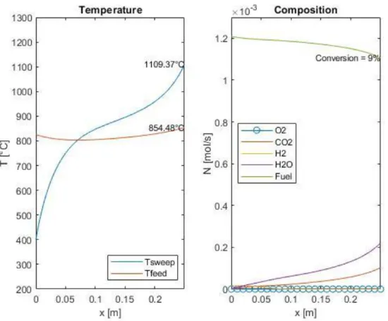
Figure 16: Example of temperature and composition profile in an OTM module, computed with the MATLAB® model ... 51

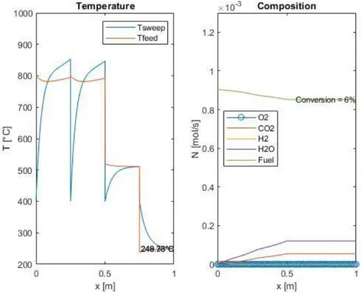
Figure 17: Two different results of the same simulation, at integration steps equal to 0.0001 and 0.01 m, respectively ... 52

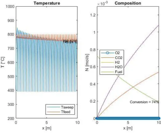
Figure 18: Two different results of the same simulation, at integration steps equal to 0.0001 and 0.1 m respectively, at milder reaction conditions ... 54

(8)

6

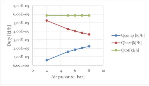
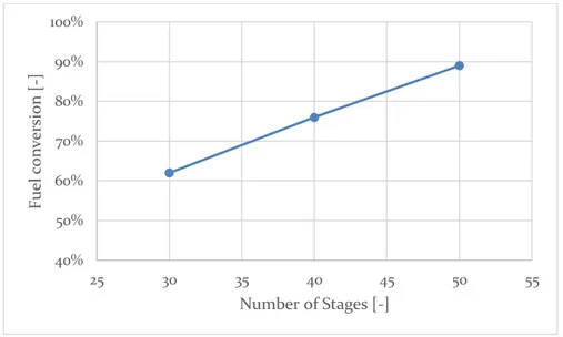
Figure 19: Loss of activity of the reactor if a pre-heating system is not implemented ... 55 Figure 20: Multistage OTM system scheme ... 56 Figure 21: Example of temperature and composition profile in an OTM module series, computed with the MATLAB® model ... 57 Figure 22: Dependence of the fuel conversion on air pressure. ... 61 Figure 23: Dependence of compression duty, heating duty and total inlet duty on air pressure ... 61 Figure 24: Dependence of the fuel conversion on the number of stages ... 62 Figure 25: Dependence of the fuel conversion on the refrigeration temperature 63 Figure 26: Dependence of the fuel conversion on the number of fluxes ... 63 Figure 27: Dependence of the fuel conversion on the air inlet temperature ... 64 Figure 28: Dependence of the fuel conversion on air quantity ... 64 Figure 29: Example of few stages to indicate the maximum reactor temperature 65 Figure 30: Dependence of the maximum reactor temperature on the number of fluxes ... 66 Figure 31: Dependence of the maximum reactor temperature on the air inlet temperature ... 66 Figure 32: Dependence of the maximum reactor temperature on air quantity .... 67 Figure 33: Dependence of net heat on the number of stages ... 68 Figure 34: Dependence of heat generation, heat need and net heat on refrigeration temperature ... 68 Figure 35: Dependence of heat generation, heat need and net heat on the number of fluxes ... 69 Figure 36: Dependence of heat generation, heat need and net heat on the air inlet temperature ... 70 Figure 37: Dependence of heat generation, heat need and net heat on the air quantity multiplicator ... 70 Figure 38: Dependence of the inlet duties on the air inlet temperature ... 71 Figure 39: Dependence of the inlet duties on the air quantity multiplicator ... 71 Figure 40: Comparison between total inlet duty and net heat production at different air inlet temperatures ... 72

(9)

7

Figure 41: Comparison between total inlet duty and net heat production at different air inlet temperatures and number of fluxes ... 72 Figure 42: Dependence of fuel conversion on the pyrolyzed plastic amount ... 73 Figure 43: Dependence of overall inlet duty and net heat production on the pyrolyzed plastic amount...74 Figure 44: Dependence of fuel conversion with the quantity of parallel reactors . 75 Figure 45: Dependence of maximum reactor temperature with the quantity of parallel reactors ... 75 Figure 46: Dependence of heat generation, heat need, and net heat produced on the quantity of parallel reactors ...76 Figure 47: Simplified plant section scheme ... 80 Figure 48: Heat integration scheme in the whole chemical recycle plant. ... 81 Figure 49: Dependence of fuel conversion on the oxygen flux multiplication factor. JO2_real = b·JO2 ... 89 Figure 50: Dependence of the fuel conversion on the height of the single chamber, keeping the total height of the OTM module constant ... 90 Figure 51: Integrated plant simulation example, with a connection between MATLAB® and ASPEN HYSYS® environments ... 92

(10)

8

List of tables

Table 1: Weight yields for polyethylene pyrolysis [kg/kg of plastics] ... 21 Table 2: Weight yields for polypropylene pyrolysis [kg/kg of plastics] ... 21 Table 3: Weight yields for polystyrene pyrolysis [kg/kg of plastics]... 21 Table 4: Molar composition of the gas stream leaving the pyrolysis section for polyethylene[%] ... 22 Table 5: Molar composition of the gas stream leaving the pyrolysis section for polypropylene [%] ... 22 Table 6: Molar composition of the gas stream leaving the pyrolysis section for polystyrene [%] ... 23 Table 7: List of compounds ... 23 Table 8: Geometrical dimensions and structural properties of a chamber ... 33 Table 9: Arrhenius constant values for oxygen transport membrane constants [55] ... 36 Table 10: Arrhenius reaction constant of the reaction rates [57] [58]: [X] is the concentration of compound X, while k = A*exp(-Ea/R/T) (see note 4) ... 39 Table 11: Parametric analysis synthesis ... 77 Table 12: Example of first guess combination of values for a gaseous stream coming from the pyrolysis of 1 kg/h of PE at 400 °C ... 78 Table 13: Example of first guess combination of values for a gaseous stream coming from the pyrolysis of 80 kg/h of PE at 400 °C ... 78

(11)

9

List of equations

( 1 ) ...24 ( 2 ) ... 27 ( 3 ) ... 27 ( 4 ) ... 34 ( 5 ) ... 35 ( 6 ) ... 35 ( 7 ) ... 36 ( 8 ) ... 37 ( 9 ) ... 37 ( 10 ) ... 37 ( 11 )... 38 ( 12 ) ... 38 ( 13 ) ... 38 ( 14 ) ... 39 ( 15 ) ... 39 ( 16 ) ... 39 ( 17 ) ... 40 ( 18 ) ... 40 ( 19 ) ... 40 ( 20 ) ... 40 ( 21 ) ... 40 ( 22 ) ... 41 ( 23 ) ... 41 ( 24 ) ...42 ( 25 ) ...42 ( 26 ) ... 43 ( 27 ) ... 43 ( 28 ) ... 43 ( 29 ) ... 43

(12)

10 ( 30 ) ... 47 ( 31 ) ... 47 ( 32 ) ... 48 ( 33 )... 48 ( 34 ) ... 48 ( 35 ) ... 48 ( 36 ) ... 59 ( 37 ) ... 59 ( 38 ) ... 59 ( 39 ) ... 75 ( 40 ) ... 82 ( 41 ) ... 82 ( 42 ) ... 83 ( 43 ) ... 83 ( 44 ) ... 83 ( 45 ) ... 83 ( 46 ) ... 84 ( 47 ) ... 85 ( 48 ) ... 85

(13)

11

Abstract

Plastic materials disposal has become a topic of outmost importance in the last few years. We are witnessing an increasing production of plastics and dependance on its usage, while the recycling techniques are almost unchanged throughout the years, with a very low recycling efficiency: around 70% of wasted plastic is being burnt or sent to landfill.

iCAREPLAST is a project funded by the European Union to implement a chemical recycling route of plastics: useful chemicals can be produced, at a very high efficiency rate, in an outlook of circular economy. Such process comprehends a preliminary pyrolysis process of all treated plastics put together, and subsequent catalytic reaction steps to obtain the desired final products.

In the pyrolysis section, also gaseous hydrocarbons are produced, which are useless for the purpose. To enhance the energetic efficiency of the process, these gases can undergo a controlled, oxy-combustion reaction, to produce a great quantity of heat to be recycled in the plant. An Oxygen Transport Membrane (OTM) reactor would help to reach high control of the reactor, high efficiency, and low volumes. Due to its nature, it is a non-conventional unit that requires a proper design process. The aim of this study is to put the basis for the design, decision-making process linked to the oxy-combustion section of such recycle plant.

Starting from the modeling of the reacting unit, it was possible to obtain feasible, numerical results as an outlet of a computational model. Then, a proper reactor configuration was hypothesized, and a qualitative, parametric study on the reactor allowed a better comprehension of the internal dynamic of the process and of the variables to be accounted for in the design process. Eventually, a plant design hypothesis brought to the formulation of the variation of the economic potential in function of such variables, a tool that can be useful in the decision-making process.

(14)

12

Sintesi

Lo smaltimento di materiale plastico è diventato un argomento di grande importanza negli ultimi anni. Assistiamo ad una crescita nella produzione di plastica, e al contempo ad una sempre crescente dipendenza dal suo utilizzo, mentre le tecniche di riciclo rimangono quasi immutate negli anni, con un’efficienza di riciclo molto bassa: circa il 70% dei rifiuti plastici viene bruciato o mandato a discarica.

Il progetto iCAREPLAST, in collaborazione con l’Unione Europea, punta a implementare un processo di riciclo chimico delle plastiche: monomeri utili vengono prodotti, con un’efficienza di riciclo molto elevata, in un’ottica di economia circolare. Tale processo prevede uno step preliminare di pirolisi di tutte le plastiche trattate complessivamente e reazioni catalitiche successive per ottenere finalmente i prodotti desiderati.

Nella sezione di pirolisi vengono prodotti anche idrocarburi gassosi non utili per il processo. Per migliorare l’efficienza energetica del processo, questi gas possono subire un trattamento controllato di ossicombustione, in modo da produrre una grande quantità di calore che può essere riciclato nell’impianto. Un reattore costituito da sistemi di Oxygen Transport Membrane (OTM) risulta funzionale allo scopo, garantendo alti livelli di controllo, alte efficienze e volumi contenuti. Data la sua natura, va disegnata opportunamente come unità non convenzionale. L’obiettivo di questo studio è mettere le basi per il processo di design e per prendere decisioni economiche per la sezione di ossicombustione di questo impianto di riciclo.

Partendo dalla modellazione del reattore, è stato possibile ottenere risultati numerici veritieri come outlet di un modello informatico. In seguito, è stata ipotizzata un’opportuna configurazione reattoristica, e uno studio parametrico qualitativo ha permesso una migliore comprensione delle dinamiche interne del processo e delle variabili da considerare nel processo di design. Infine, un’ipotesi di design dell’impianto ha portato alla formulazione della variazione del potenziale economico in funzione di tali variabili, uno strumento che può essere utile per prendere decisioni economiche.

(15)

13

1. Introduction

1.1 Plastic demand: an increasing issue

Plastic materials disposal has become a topic of utmost importance in the last few years. This issue is related to the yearly increasing production of plastics worldwide (Figure 1). In 2018 only, 359 million tons of plastics were produced worldwide, of which 61.8 Mt in Europe: plastics are extensively used in the sectors of packaging, consumer and household goods, and constructions [1].

Figure 1: Yearly Plastics Production [2, 3, 4, 5]

In Europe in 2018, 29.1 Mt of plastic were collected to be disposed of, of which 17.8 Mt (62% of the total) were coming from packaging waste [1] – everyday life waste. A huge problem of environmental pollution arises from its incorrect disposal: of all the plastic waste in a year in Europe, only 32.5% was recycled in 2018 [6].

Since 2006, the total quantity of plastic waste sent to recycling facilities increased twofold (Figure 2). Nevertheless, although landfilled quantities decreased by 44% compared to 2006, with an average annual fall rate of 4.7%, 7.2 Mt of plastic waste still ended up in landfill in 2018 [6].

230 257 279 288 299 311 322 335 348 359 61 65 59 59 57 59 58 60 64,4 61,8 0 50 100 150 200 250 300 350 400 2005 2007 2011 2012 2013 2014 2015 2016 2017 2018 P la st ic P ro d u ct io n [ M t] Year World Europe

(16)

14

Figure 2: Waste treatment options for post-consumer plastic waste 2006-2018 in EU28+2 [6]

When it comes to packaging waste, the situation changes (Figure 3). The quantity of packaging plastic waste sent to landfill decreased by 54% compared to 2006 and recycled plastic increased by more than 92% [6]. This shows that in the European Union the importance of a correct waste treatment, like for instance a correct sorting practice, has been emphasized, and eventually the capacity of the recycle facilities was enhanced.

Figure 3: Waste treatment options for post-consumer plastic packaging waste 2006-2018 in EU28+2

1.2 Plastic recycling state of the art

Plastic recycling techniques improved increasingly due to the exponentially increasing amount of plastic to be treated worldwide. These can be divided in four types mainly (Figure 4) [7]:

- Primary recycle, which consists of simple cleaning procedures to use a piece of plastic with the same features of the end use polymer [7].

(17)

15

Figure 4: Various approaches for recycling plastic solid waste [7]

- Secondary recycle, also called mechanical recycle. The preliminary operations preceding this process are schematized below (Figure 5):

Figure 5: Preliminary operations to secondary recycle [7]

It can be carried via palletizing, extrusion (the most common in polymeric film production), injection molding, drawing, and shredding.

- Tertiary recycle involving chemical reactions, in particular catalytic paths, energy recovery processes and thermolysis.

(18)

16

The main recycle route currently used in Europe is mechanical recycle, with just 0.1 Mt undergoing chemical recycling. Of course, mechanical recycle has some efficiency, as for instance the recycling rate for packaging plastics lowers from 42% to 29% when the preliminary procedures are applied (Figure 6). This means that the remainder is sent to landfill (27%) or incinerated for energy recovery (42%).

Figure 6: Estimated packaging recycling rate change due to preliminary operations [6]

A large part of the efficiency of the process is being detracted by the sorting procedure: plastic waste must be sorted by polymer type and these are to be treated separately. This affects the overall process by making multilayer plastic packaging, constituted by layers made of different polymers, unrecyclable.

1.3 iCAREPLAST: a game-changing technology

In the European plastic-disposal scenario, a project took life from the cooperation of the Consejo Superior de Investigaciones Científicas (CSIC) and several partners from all over the European Community, including companies and universities. Its

(19)

17

name is iCAREPLAST, acronym for Integrated Catalytic Recycling of Plastic

Residues into Added-Value Chemicals [8].

Figure 7: iCAREPLAST logo [8].

The purpose of the project is demonstrating a whole new plastic waste valorization technology in a pilot plant able to process more than 80 kg/h of plastic. The plastic to be treated will undergo a tertiary recycle process, comprising a thermolysis (pyrolysis) section and some catalytic reactions that will lead to the production of alkylbenzenes and BTX – very valuable chemicals [8].

Figure 8: Overall Concept behind iCAREPLAST Process [8]

The main sections of the plant are (Figure 8):

- The pyrolysis section, in which plastics are burnt and melted to be converted to smaller, useful molecules. Besides, a gas current and a carbon char current leave the section.

- The alkylation section and the hydrogenation one, which consist of sequential catalytic steps.

(20)

18

- The fractionation section, from which it is possible to obtain the products of interest and a lighter gas current.

- The oxy-combustion section, where gases leaving the pyrolysis section and the fractionation section are converted to a more valuable CO2 current.

The main advantages of such recycling route are:

- Any plastic waste can undergo pyrolysis: this means that the amount of recyclable plastics could increase, avoiding landfill waste amassing and waste incineration. As a proof of this, the purpose of the iCAREPLAST project is to treat 250,000 t of plastic waste which otherwise, due to the currently available technologies, would become landfill [8].

- The products obtained from the process can be used for many purposes, in the petrochemical and fine chemical industries (such as detergent and surfactant industries), and also for polymers production, to enhance plastics circular economy (Figure 9).

(21)

19

- The polymers produced starting from the obtained products will be

virgin-quality polymers, unlike currently recycled plastics – for instance, in

Europe the use of functional barriers in multilayer polymers in contact with food is mandatory when a recycled polymer is used, to meet the requirements stated by the European Commission in terms of food contamination [9].

- Subproducts of the process like CO2 and char are recovered and valorized

to maximize the yield of the process, reduce the environmental footprint, and ensure economic sustainability [8].

1.4 Gas recovery and the oxy-combustion section

In the frame of iCAREPLAST project, a series of tests was executed in the pyrolysis pilot section in order to characterize the resulting pyrolytic streams. The weight yield of liquid, gas, and solid products per kg of plastic was obtained from theoretical models [10] [11] [12] [13] [14] [15] [16] [17] [18] [19] [20] [21] [22] [23] [24] [25] [26] [27] [28] [29] [30] [31] [32] [33] [34] [35] and adapted to experimental results, at different pyrolysis temperatures for each kind of plastic treated: polyethylene (Table 1: Weight yields for polyethylene pyrolysis [kg/kg of plastics]), polypropylene (Table 2), and polystyrene (Table 3).

The liquid stream is the one of main interests for the iCAREPLAST process, while the solid stream is substantially a carbon char stream and the gaseous stream contains light hydrocarbons. Also, the gaseous stream composition was analyzed for each current (Table 4: Molar composition of the gas stream leaving the pyrolysis section for polyethylene[%], Table 5, Table 6).

Hydrocarbons leaving the pyrolysis section in the gaseous stream range from 1 to 6 carbon atoms, and (usually) the fraction of lighter hydrocarbons increases with the pyrolysis temperature, which is between 400 and 500 °C. It also contains a small fraction of hydrogen.

This gas fraction is useless for the subsequent process, whose aim is to produce alkylbenzenes and BTX which have at least 6 carbon atoms: Therefore, this fraction has been valorized in the process to obtain heat in an oxy-combustion process, a

(22)

20

combustion carried in presence of oxygen only, instead of air. The oxy-combustion approach also allows to separate the CO2 generated in the combustion reactions.

(23)

21

Table 1: Weight yields for polyethylene pyrolysis [kg/kg of plastics]

T (°C) 400 410 420 430 440 450 460 470 480 490 500

Liquid 82.39 84.23 85.65 86.64 87.24 87.41 87.17 86.50 85.42 83.93 82.02

Gas 16.69 14.63 12.99 11.80 10.96 10.57 10.59 11.04 11.90 13.17 14.87

Solid 0.92 1.14 1.36 1.56 1.80 2.02 2.24 2.46 2.68 2.90 3.12

Table 2: Weight yields for polypropylene pyrolysis [kg/kg of plastics]

T (°C) 300 325 350 375 400 425 450 475 500 525 550 575 600 625 650 675 700

Liquid 52.00 61.56 69.75 76.56 82.00 86.06 88.75 90.06 90.00 88.56 85.75 81.56 76.00 69.06 60.75 51.06 40.00 Gas 14.17 13.35 11.65 9.64 7.77 6.35 5.63 5.77 6.91 9.14 12.55 17.18 23.07 30.24 38.74 48.56 59.72 Solid 33.83 25.09 18.60 13.79 10.23 7.58 5.62 4.17 3.09 2.29 1.70 1.26 0.93 0.69 0.51 0.38 0.28

Table 3: Weight yields for polystyrene pyrolysis [kg/kg of plastics]

T (°C) 350 375 400 425 450 475 500 525 550

Gas 3.0622 7.3886 6.3953 5.0478 5.7613 9.7621 17.6979 29.9221 46.6338

Liquid 47.6550 64.9863 77.5300 85.2863 88.2550 86.4363 79.8300 68.4363 52.2550

(24)

22

Table 4: Molar composition of the gas stream leaving the pyrolysis section for polyethylene[%]

T H2 CH4 C2H4 C2H6 C3H6 C3H8 C4H10(ISO) C4H8 C4H10(N) C4H8 C4H6 C5H10 C6H12 400 4.0098 16.4499 6.5985 15.3848 10.0217 10.6061 0.3515 4.1668 4.4155 24.8553 1.2946 1.1602 0.6853 410 4.7987 15.6665 6.2843 14.6522 9.5445 10.1010 0.3700 4.3862 4.6479 26.1635 1.3628 1.2611 0.7614 420 5.3392 14.9205 5.9850 13.9545 9.0900 9.6200 0.3895 4.6170 4.8925 27.5405 1.4345 1.3708 0.8460 430 4.7400 14.2100 5.7000 13.2900 9.0900 9.6200 0.4100 4.8600 5.1500 28.9900 1.5100 1.4900 0.9400 440 5.0010 13.6416 5.5860 13.0242 8.9082 9.4276 0.4182 4.9572 5.2530 29.5698 1.5402 1.6390 1.0340 450 4.9107 13.3688 5.4743 12.7637 8.7300 9.2390 0.4266 5.0563 5.3581 30.1612 1.5710 1.8029 1.1374 460 4.7567 13.1014 5.3648 12.5084 8.5554 9.0543 0.4351 5.1575 5.4652 30.7644 1.6024 1.9832 1.2511 470 4.5365 12.8394 5.2575 12.2583 8.3843 8.8732 0.4438 5.2606 5.5745 31.3797 1.6345 2.1815 1.3763 480 4.2471 12.5826 5.1523 12.0131 8.2166 8.6957 0.4527 5.3658 5.6860 32.0073 1.6672 2.3997 1.5139 490 3.8854 12.3309 5.0493 11.7728 8.0523 8.5218 0.4617 5.4731 5.7997 32.6474 1.7005 2.6396 1.6653 500 3.4478 12.0843 4.9483 11.5374 7.8913 8.3514 0.4710 5.5826 5.9157 33.3004 1.7345 2.9036 1.8318

Table 5: Molar composition of the gas stream leaving the pyrolysis section for polypropylene [%]

(25)

23

Table 6: Molar composition of the gas stream leaving the pyrolysis section for polystyrene [%]

Table 7: List of compounds

Compounds Compounds

H2 hydrogen C4H10(ISO) iso-butane

CH4 methane C4H8 1-butene C2H4 ethylene C4H10(N) n-butane C2H6 ethane C4H8 2-butene C3H6 propylene C4H6 1,2-butadiene C3H8 propane C5H10 1-pentene C6H12 1-hexene

(26)

𝐶_𝑛𝐻_𝑚+ (𝑛 +𝑚

4)𝑂2 → 𝑛𝐶𝑂2+ 𝑚

2 𝐻2𝑂

( 1 )

For each mole of a hydrocarbon of length n, n moles of carbon dioxide are generated.

The main reasons to perform an oxy-combustion process on such gaseous stream are:

- An incredible quantity of heat can be recovered with a combustion reaction: for instance, methane has a heating value of 55,4 MJ/kg. This heat can be recycled in the plant, to lower operational costs and enhance the thermal efficiency of the whole process: this is achieved by using the produced heat in the pyrolysis reactor, as well as heat exchangers in the plant, or for production of electric energy useful for the operation of the plant.

- The gas leaving the pyrolysis section is useless, while carbon dioxide can be easily stored and used for many purposes, for instance:

o In a Fischer-Tropsch plant [36] to produce clean fuel

o In the food industry, as a food preservative and to produce carbonated beverages

o As a fire extinguisher

- Besides being useless, this gaseous current is potentially dangerous, if it comes in contact with oxygen in an uncontrolled environment. Burning it to CO2 prevents uncontrolled explosion of the gases and, if stored correctly,

takes the mixture out of its explosive limits.

The main problem with combustion is that it is a runaway reaction1_{so it must be}

carried out in very well controlled conditions not to lead to dangerous outcomes, obtaining the desired result. Of course, being in an oxy-combustion environment rather than a regular combustion one increases such risk, because the nitrogen contained in air would act as an inert and lower the temperature, but it would also

1_{Runaway reactions are highly exothermic reactions, characterized by very high reaction rates and} a very high (and rapid) increase in temperature, so that they are very difficult to control. For instance, the reaction rate for the methane combustion (section 3.3) is 5.2461e+9 [s^(-1)].

(27)

25

increase by around 4 times the volume of the reactor, due to the air proportions between oxygen and nitrogen. Also, the presence of an inert gas acting as a third

body could lower the temperature of the gases, lowering the possibility of heat

recycling in the plant. Moreover, performing an oxy-combustion process nullifies the possibility of NOx production, which can cause environmental pollution.

The reaction can be controlled by:

- Injecting oxygen gradually, to avoid explosion. In this sense, a controlled injection of oxygen only rather than air would be more precise for the lower volumes to be treated.

- Cool down the reacting system while the reaction takes place, to avoid crossing the maximum reactor admissible temperature.

1.5 Oxy-combustion reactor: KERIONICS Oxygen

Transport Membrane system

A way of achieving a controlled oxygen injection by considering an oxy-combustion approach in the reacting system was provided by the company KERIONICS, which produces Oxygen Transport Membrane (OTM) systems.

An OTM system consists of membrane structures made of ceramic materials presenting mixed ionic-electronic conductivity (MIEC) which allows a 100% selective oxygen separation. This is due to the ability of MIEC materials to diffuse oxygen in the ionic form O2_{- through the oxygen vacancies present in the material’s}

crystal lattice

At high temperatures (>600 ºC), OTM technology has been demonstrated as an appealing option for the in-situ O2 production in medium and small-scale

applications. The main reasons are the high O2 purity that can be obtained and the

reduction in pure O2 production costs of up to a 35% with respect to conventional

technologies, such as cryogenic air distillation and Pressure Swing Adsorption (PSA) [37].

(28)

26

Furthermore, OTMs can reduce energy consumption and enhance overall plant efficiency due to the synergic thermal integration they provide [37]. At the same time, the use of OTMs result in more efficient and environmentally sustainable processes: this is due to the fact that by conducting combustions with pure O2, then only CO2 and H2O are generated and the capture and storage of the generated CO2 is enabled, along with a drastic reduction in CO2 emissions.

Typically, OTMs consider high permeating materials such as perovskites. The mineral itself named perovskite is a titanate with the formula CaTiO3, but it is part

of a supergroup of minerals having different compositions but the same, octahedral structure [38]. For a so called stoichiometric perovskite, the general formula is ABX3, where A and B are large cations and X could be oxygen, but also fluorine (in

fluoride perovskites) or large metalloids like nickel [38]. However, there are several non-stoichiometric perovskites with more complex formulas [38]. Amongst perovskites, the best performing material is Ba0.5Sr0.5Co0.8Fe0.2O3-d, even if its low

stability avoids its consideration for applications where reducing and CO2

-containing atmospheres can be met.

Other considered materials are the fluorites. Fluorites are a class of minerals with the formula MX2: the common mineral fluorite is MX2, but many compounds adopt

this structure, like for instance BaF2, PuO2 and ZrO2 [39]. They take a tetrahedral

shape where the M element form a face-centered cubic (FCC) structure while the X element occupy the tetrahedral interstitial sites [39]. These materials present a higher stability when exposed to the mentioned environments; however, the lack of electronic conductivity result in poor permeation fluxes.

A solution is the use of composites or dual-phase materials, by combining a material presenting ionic conductivity with another presenting electronic conductivity, and both being stable under the considered environments, although stable MIEC materials can also be considered. There are many possible combinations of materials suitable for constituting a dual-phase material: ceramic-metal composites [40] [41] [42], fluorite-spinel [43] [44] [45], perovskite-spinel [46] and perovskite-fluorite [47].

(29)

27

Figure 10: Structure of the ideal perovskite [38] and fluorite [48].

Oxygen contained in air undergoes an electrochemical process in contact with the membrane, so that it passes selectively through the membrane while letting nitrogen flow. The reaction mechanism is schematized below (Figure 11Figure 1): Usually when dealing with OTMs, the chamber where air passed is referred to as the feed chamber, while the sweep chamber is the one where any other gas passes.

The steps in the scheme represent the main resistances to the flux of oxygen [49]:

i. Oxygen diffusion from the feed stream to the membrane surface. ii. Oxygen adsorption on the membrane surface at the feed side. iii. Dissociation surface exchange reaction:

𝑂2+ 4𝑒− → 2𝑂2− ( 2 )

iv. Incorporation of the oxygen ion into membrane crystalline structure.

v. Ion diffusion through the membrane oxygen vacancies (and electron counter-diffusion through electronic bands).

vi. O2-_{adsorption on the membrane surface at the sweep side}

vii. Recombination surface exchange reaction:

2𝑂2− _{→ 𝑂}

2+ 4𝑒− ( 3 )

viii. Oxygen molecule desorption from the membrane surface

(30)

28

Figure 11: Simplified scheme of OTM process [50]

Coupling the quantitative information about the oxygen flux across the membrane with the one concerning the reacting system, it is possible to model an OTM oxy-combustion reactor.

1.6 Object of the thesis

For every kg of plastic processed, the iCAREPLAST plastic chemical recycle plant pyrolysis section produces between 5 and 20 kg of gases, depending on the type of processed plastic, and on temperature (Table 1: Weight yields for polyethylene pyrolysis [kg/kg of plastics], Table 2,Table 3). A safe, environmental-friendly, but also economically suitable solution must be implemented to dispose of this gas current and make a profit from it, in terms of energy recovery and value of the obtained products.

Oxy-combustion seems the most convenient solution, but it must be designed and controlled carefully, to monitor production and to avoid dangerous outcomes. A

(31)

29

membrane system is available for the task, to inject oxygen in the reacting system in a controlled way.

The former object of the thesis is to model a membrane reactor for the task and obtain information about conversion and temperatures of the currents leaving the system by implementation of the model in a script and numerical integration.

Also, once a precise, satisfyingly smooth computer model is created, it is possible to obtain quantitative results. The latter object of the thesis is to use this information to perform an economic assessment of the oxy-combustion section of the plant: it consists in a parametric study of the system, in order to identify the

(32)

30

2. Materials, tools, and methods

A simplified scheme of the development of the thesis is depicted below (Figure 12):

Figure 12: Scheme of the thesis

First of all, the model is created theoretically, with the support of articles and books found in literature about the thermodynamics and kinetics of the system.

Then, the theoretical model is implemented in MATLAB® to perform a numerical integration. The following data is used:

- Information about weight yields and composition of the gas stream leaving the pyrolysis section, available from iCAREPLAST (Table 1: Weight yields for polyethylene pyrolysis [kg/kg of plastics], Table 2,Table 3,Table 4: Molar composition of the gas stream leaving the pyrolysis section for polyethylene[%], Table 5, Table 6).

- Information about the membrane material and structure, available from KERIONICS (Table 8), such as:

o Dimensions of the membrane

o Heat conductivity and heat capacity of the membrane o Maximum allowed temperature and pressure

o Dimensions of the whole structure

- Information about the oxygen transport mechanism, available from literature and applied to the specific membrane system.

- Thermodynamic values for the compounds involved in the system [51]. - Target values of conversion requested by iCAREPLAST.

(33)

31

Once the quantitative results are obtained from the software, these are coupled to new data, generated using ASPEN HYSYS®2_{, related to other pieces of equipment}

in the oxy-combustion plant section. These data are used to perform a parametric study of the plant section, using Microsoft Office Excel®.

Eventually a theoretical model for the calculation of the economic potential is created, considering the whole study and the needs of the two companies.

2_{Aspen HYSYS® is a plant simulation environment where the performance of the plant can be} evaluated, including various tools like fluid EoS packages and thermodynamics, various equipment simulation, but also calculation of investment cost and duties expenses.

(34)

32

3. Theoretical model of the OTM reactor

The aim is to obtain a mathematical model being:

- Based on solid hypotheses, to make the equations as slim as possible, - Detailed in the definition of each term of the equations,

- As generical as possible, to comply with any given input data for the reactor.

3.1 Choice of the type of reactor

The information given by the company making the OTM system available is used to make a simplified reactor model. The membrane system that will be considered is constituted by modules: the structure of a single module is described below (Figure 13):

Figure 13: OTM module structure and dimensions

The OTM module is constituted by a series of superposed membranes, which divide the air flow from the pyrolysis gas flow This superposition makes sure that various chambers are created, between which each stream can divide and through

(35)

33

which it can flow, enhancing mass and heat transfer due to the much lower height of each chamber with respect to the whole module.

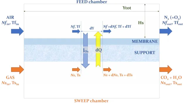
A simple scheme of the reaction environment (Figure 14), composed by two

chambers separated by a membrane, will allow a better understanding of the choices taken in the modeling process, the definition of the dimensions of the chambers, and the structure of the membrane.

Figure 14: Scheme of the reaction environment and dimensions of a chamber (in green)

Quantitative values for the membrane are listed below (Table 8).

Table 8: Geometrical dimensions and structural properties of a chamber

Dimension Description Value

Hs Height of the single

chamber

2 [mm]

z Width 25 [cm]

Ytot Total length 25 [cm]

Tmax Maximum temperature allowed

900 [°C]

Pmax Maximum pressure allowed

8 [bar]

L Dense membrane layer 20 [μm]

Lsupp Porous membrane layer 2 [mm]

ksupp Heat conductivity of the

porous support

(36)

34

Usually, OTM systems are composed by a thick membrane layer and a porous support layer (Figure 14).

If the overall structure of the module is considered, the total height H (Figure 13) will depend on the number of membranes in a single modulus:

𝐻 = (𝐿 + 𝐿_{𝑠𝑢𝑝𝑝}) ∗ 𝑁_{𝑚𝑒𝑚𝑏𝑟𝑎𝑛𝑒𝑠}+ 𝐻_𝑠 ∗ (𝑁_{𝑚𝑒𝑚𝑏𝑟𝑎𝑛𝑒𝑠}+ 1) ( 4 ) Where Nmembranes is the number of membranes in the reactor.

The height of a single chamber Hs is lower by 2 orders of magnitude than the total length Ytot and the width z. If the aim is to model just the part of the reactor that is sufficiently far from the inlet and outlet section (where some turbulence will occur due to the splitting of the stream and the change of direction of the fluid), we can assume for the sake of simplicity that the flow is homogeneous along the dimensions of the height Hs and the width z, and that it varies only along the coordinate of length Y.

In fact, the velocity along this coordinate will be much higher due to both the forced direction of the flow and the low transversal area. So, this is the only coordinate that will be investigated, using a plug flow model. The result will be a modified Plug Flow Reactor (PFR), with the difference that the contribution of mass transfer should be considered in the equations as well.

A co-current configuration is represented in the scheme (Figure 14): this is the one

that is taken in consideration. A countercurrent configuration is discarded immediately due to the nature of the reactions involved, which require a good control of temperature. In fact the gas at the inlet of the reactor, characterized by high reaction rates when in contact with oxygen due to the maximum possible concentration of reagents, exchanges heat with the air that has already been heated up by combustion: a hotspot3_{can take place inside the reactor. The temperature in}

a hotspot can be higher than the maximum temperature allowed; moreover, it is

(37)

35

very difficult to control using the available variables (like the temperature of the air at the opposite side of the reactor, which is its inlet), and it can lead to runaway conditions in a very short time.

The mass and heat balance equation will be written by making a steady state balance in an infinitesimal slice of the reacting environment composed by the two chambers and the membrane, of length dY (Figure 14) [52]. Pressure drops are

neglected in first approximation, to simplify the model.

3.2 Mass balance equations

If we state that Ncomp is the number of components in the gas stream, there will be Ncomp + 2 mass balance equations to be built.

Considering the sweep chamber, the mass balance equations are so structured (t is the time coordinate):

𝑑𝑛_𝑠,𝑖

𝑑𝑡 = 𝑁𝑠,𝑖− (𝑁𝑠,𝑖+ 𝑑𝑁𝑠,𝑖) + 𝑏𝑖𝑑𝑁𝑜𝑥,𝑓𝑙𝑜𝑤 + 𝑑𝑁𝑟 = 0, [mol/s] ( 5 ) Where:

- ns,i = moles of component i in the sweep chamber slice [mol]

- Ns,i = stream of component i entering the sweep chamber slice [mol/s]

- Ns,i + dNs,i = stream of component i leaving the sweep chamber slice [mol/s]

- bi = Boolean operator being

o 0, if i ≠ oxygen o 1, if i = oxygen

- dNox,flow = quantity of oxygen flowing per unit of time through the

membrane [mol/s]. it is equal to:

𝑑𝑁𝑜𝑥,𝑓𝑙𝑜𝑤 = 2 ∗ 𝐽𝑂2∗ 𝑧 ∗ 𝑑𝑌, [mol/s] ( 6 )

Where JO2 is the oxygen flux across the membrane.

The system that has been considered in this work is made of a mixture of a perovskite, La0.6Sr0.4Co0.2Fe0.8O3-δ (LSCF) and a fluorite, Ce0.9Gd0.1O1.95-δ (CGO)

(38)

36

of membrane, the main resistances detected to the flux of oxygen are the surface reactions [53]. Due to this, the oxygen flux can be represented by a single formula [54]: 𝐽_𝑂2 = 𝐷𝑣𝑘𝑟(𝑃 ′ 𝑂2 0.5 − 𝑃′′ 𝑂2 0.5 ) 2𝐿𝑘𝑓(𝑃′𝑂2𝑃 ′′ 𝑂2) 0.5 + 𝐷𝑣(𝑃′𝑂2 0.5_{+ 𝑃}′′ 𝑂2 0.5₎, [mol/m^2/s] ( 7 ) Where:

- JO2 = molar flux of oxygen per membrane surface

- Dv = oxygen vacancy bulk diffusion coefficient [m^2/s], with an Arrhenius

type dependency on temperature4_.

- kf, kr = forward and reverse Arrhenius4 reaction rate constants for the

dissociation reaction (eq. ( 2 )) - L = membrane thickness

- P’O2 = partial pressure of oxygen in the feed side [atm]

- P’’O2 = partial pressure of oxygen in the sweep side [atm]

The values of the constant defining Dv, kf, and kr [55] are listed below (Table 9):

Table 9: Arrhenius constant values for oxygen transport membrane constants [55]

Arrhenius constant A*exp(-Ea/R/T)

A Ea [J/mol]

Dv 1.01e-6 [m^2/s] 7.56e+4

kf 9.21e+6 [m/atm^0.5/s] 2.68e+5

kr 1.75e+15 [mol/m^2/s] 3.77e+5

The formula reflects the dependence of the oxygen flux on temperature, membrane thickness, and oxygen gradient difference between the two chambers. Due to the very low thicknesses usually involved, the temperature used in the equation is the

4_{An Arrhenius dependency on temperature takes the shape k(T) = A*exp(-Ea/R/T) where A is called}

(39)

37

air stream temperature. The whole flux is multiplied by 2 to consider the heat flux from above and below.

- dNr = quantity of component i generated per unit time due to the reactions

occurring. It is equal to:

𝑑𝑁𝑟 = ( ∑ 𝜈𝑖,𝑗𝑟𝑗 𝑁𝑟𝑒𝑎𝑐𝑡

𝑗=1

) ∗ 𝐴_𝑡∗ 𝑑𝑌, [mol/s] _{( 8 )}

Where

o Nreact = number of total reactions

o νi,j = stoichiometric coefficient for component i in reaction j, positive

if i is a product and negative if it is a reactant

o rj = j-th reaction rate, function of gas temperature and composition5

[mol/m^3/s]

o At = transversal area of the chamber = Hs*z

By inserting equations ( 6 ) and ( 8 ) in equation ( 5 ), and dividing by dY, we obtain:

𝑑𝑁_𝑠,𝑖

𝑑𝑌 = 𝑏𝑖 ∗ 𝐽𝑂2∗ 𝑧 + ( ∑ 𝜈𝑖,𝑗𝑟𝑗

𝑁𝑟𝑒𝑎𝑐𝑡 𝑗=1

) ∗ 𝐴_𝑡 for i = 1…Ncomp [mol/s] ( 9 ) For the components in the feed chamber, oxygen and nitrogen, material balances are simpler because no reactions occur.

For oxygen:

𝑑𝑛_𝑓,𝑂₂

𝑑𝑡 = 𝑁𝑓,𝑂2 − (𝑁𝑓,𝑂2 + 𝑑𝑁𝑓,𝑂2) − 𝑑𝑁𝑜𝑥,𝑓𝑙𝑜𝑤 = 0, [mol/s] ( 10 ) Where:

- nf,O2 = moles of oxygen in the feed chamber slice [mol]

- Nf,O2 = stream of oxygen entering the feed chamber slice [mol/s]

5_{A reaction rate is usually in the form r = k(T)*f(C), where k(T) depends on temperature in an} Arrhenius fashion, and f(C) is a function of the array of concentrations of the species in the system. A common shape for f is ∏ 𝐶𝑖𝛼𝑖,𝑗

𝑁𝑐𝑜𝑚𝑝

𝑖=1 where αi,j is the order of reaction j for the component i; it is

(40)

38

- Nf,O2 + dNf,O2 = stream of oxygen leaving the feed chamber slice [mol/s]

By using equation ( 6 ) and simplifying:

𝑑𝑁𝑓,𝑂2

𝑑𝑌 = −𝐽𝑂2∗ 𝑧 [mol/s]

( 11 )

Since nitrogen does not flow nor react, its mass balance equation is trivial (Nf,N2 is

the nitrogen stream in the feed chamber slice):

𝑑𝑁_𝑓,𝑁₂

𝑑𝑌 = 0 [mol/s] ( 12 )

3.3 Reaction set: simplifications using the LHV

As stated before, the gas stream contains a great variety of compounds: all of these undergo combustion when in contact with oxygen, at very high reaction rates6_.

Since:

- the very interest of this thesis is to evaluate the quantity of carbon dioxide formed and the generated heat

- the speed and stability of the script has to be considered

- a single reaction set including all species is difficult to find in literature, and for the sake of the reliability of the model it is risky to combine different reaction sets coming from different studies – at different reaction conditions

The model is simplified by assuming a pseudo-composition of gases, where at the beginning only hydrogen and methane are present. This was done by converting the moles of the remaining hydrocarbons into their methane equivalent using their

lower heating value (LHV)7_[56]:

𝑛_𝑖𝐶𝐻4,𝑒𝑞 _{= 𝑛}

𝑖 𝐿𝐻𝑉𝑖

𝐿𝐻𝑉_𝐶𝐻4 [mol/s] ( 13 )

This way, the equivalent number of moles takes into account the number of carbon atoms in the chain and the heat that is generated from combustion. The total

6_{For instance, at T = 400°C the Arrhenius constant for methane oxycombustion is 8.8104*10^10 1/s.} 7_{A measure of the heat produced by combustion of a mole of fuel.}

(41)

39

amount of methane theoretically entering in the system is given by the sum of the methane equivalent for each compound, plus the actual amount of methane contained in the mixture.

The reaction set becomes much simpler. It is constituted by just two reactions: methane combustion [57] and formation of water from hydrogen [58]:

𝐶𝐻4+ 2𝑂2 → 𝐶𝑂2+ 2𝐻2𝑂 ( 14 )

𝐻₂+1

2𝑂2 → 𝐻2𝑂

( 15 )

The values of the Arrhenius reaction constants are listed below (Table 10):

Table 10: Arrhenius reaction constant of the reaction rates [57] [58]: [X] is the concentration of compound X, while k = A*exp(-Ea/R/T) (see note 4)

Reaction Reaction rate A Ea

Eq ( 14 ) k*[CH4]-0.3[O2]1.3 8.3e+5 [1/s] 30 [kcal/mol]

Eq ( 15 ) k*[H2][O2]0.5 5.69e+11

[(m^3/kmol)^(1/2)/s]

1.468e+8 [J/kmol]

Regardless of the composition of the gaseous stream, the most abundant product is water: this requires a separation section downstream, for instance a flash unit for water condensation.

3.4 Heat balance equations

Two heat balance equations must be written, one on the sweep side and one on the feed side. Ts is the temperature in the sweep chamber while Tf the one in the

feed chamber.

Considering the sweep side, the heat balance will be:

𝑑𝐻̂_𝑠

𝑑𝑡 = 𝐻̇𝑠− (𝐻̇𝑠+ 𝑑𝐻̇𝑠) + 𝑑𝐻̇𝑜𝑥,𝑓𝑙𝑜𝑤− 𝑑𝑄̇ = 0, [W] ( 16 ) Where:

(42)

40

- 𝐻̇𝑠 = enthalpy flux related to the gas stream entering the sweep chamber

slice. It can be expressed as:

𝐻̇_𝑠 = ∑ 𝑁_𝑠,𝑖∗ ℎ_𝑖(𝑇𝑠), [W]

𝑁𝑐𝑜𝑚𝑝 𝑖=1

( 17 )

Where hi(Ts) is the molar enthalpy of component i in function of

temperature, which (if residual enthalpies are neglected, [52]) can be rewritten as: ℎ_𝑖(𝑇𝑠) = ℎ_𝑖(𝑇𝑟𝑒𝑓) + ∫ 𝑐_𝑝,𝑖𝑣 _(𝑇) 𝑇𝑠 𝑇𝑟𝑒𝑓 𝑑𝑇_𝑠, [J/mol] ( 18 ) Where:

o Tref = reference temperature (298 K)

o hi(Tref) = enthalpy of formation of component i at the reference

temperature at the gas state [J/mol]

o cp,iv(T) = heat capacity of component i, in function of temperature

[J/mol/K]

- 𝐻̇𝑠+ 𝑑𝐻̇𝑠 = enthalpy flux related to the gas stream leaving the sweep

chamber slice [W]. Using equations ( 17 ) and ( 18 ), the derivative in equation ( 16 ) is soon calculated:

𝑑𝐻̇_𝑠 =𝜕𝐻̇𝑠 𝜕𝑇 𝑑𝑇 + ∑ 𝜕𝐻̇_𝑠 𝜕𝑁_𝑠,𝑖𝑑𝑁𝑠,𝑖 = ∑ 𝑁𝑠,𝑖𝑐𝑝,𝑖 𝑣 _{(𝑇)𝑑𝑇 + 𝑑𝑁} 𝑠,𝑖ℎ𝑖(𝑇𝑠) 𝑁𝑐𝑜𝑚𝑝 𝑖=1 𝑁𝑐𝑜𝑚𝑝 𝑖=1 ( 19 )

- 𝑑𝐻̇_{𝑜𝑥,𝑓𝑙𝑜𝑤} = enthalpy flux related to the oxygen flux across the membrane, expressed as:

𝑑𝐻̇𝑜𝑥,𝑓𝑙𝑜𝑤 = 𝐽𝑂2∗ 𝑧 ∗ 𝑑𝑌 ∗ ℎ𝑂2(𝑇𝑓), [W] ( 20 ) - dQ̇= heat transfer contribution, positive when flowing from the sweep

chamber to the feed chamber, equal to:

𝑑𝑄̇ = 2 ∗ 𝑈 ∗ ∆𝑇 ∗ 𝑧 ∗ 𝑑𝑌 [W] ( 21 )

(43)

41

o U = global heat transfer coefficient [W/m^2/K], whose shape will be discussed below (see 3.5).

o ∆T = Ts – Tf = temperature drop across the membrane [K]

It is multiplied by 2 to consider the heat flux from above and below.

Using equations ( 9 ), ( 16 ), ( 17 ), ( 18 ), ( 19 ), ( 20 ) and ( 21 ) the heat balance is obtained: 𝑑𝑇_𝑠 𝑑𝑌 = 𝐽_𝑂₂𝑧 ∫ 𝑐𝑝,𝑂2 𝑣 _{(𝑇)𝑑𝑇 − ∑} _∑ _𝜈 𝑖,𝑗𝑟𝑗 𝑁𝑟𝑒𝑎𝑐𝑡 𝑗=1 𝑁𝑐𝑜𝑚𝑝 𝑖=1 𝑇𝑠 𝑇𝑓 𝐴𝑡ℎ𝑘(𝑇𝑠) − 𝑈∆𝑇𝑧 ∑ 𝑁𝑠,𝑖𝑐𝑝,𝑖𝑣 𝑁𝑐𝑜𝑚𝑝 𝑖=1 (𝑇𝑠) ( 22 )

Three main contributions can be distinguished in the equation: one related to the oxygen flux across the membrane, one related to the heat of reaction8_{, and one}

related to the heat flux across the membrane.

The heat balance in the feed chamber has the same structure:

𝑑𝐻̂𝑓

𝑑𝑡 = 𝐻̇𝑓− (𝐻̇𝑓+ 𝑑𝐻̇𝑓) − 𝑑𝐻̇𝑜𝑥,𝑓𝑙𝑜𝑤 + 𝑑𝑄̇ = 0, [W] ( 23 ) Where:

- 𝐻̂_𝑓 = enthalpy in the feed chamber slice [J]

- 𝐻̇_𝑓 = enthalpy flux related to the gas stream entering the feed chamber slice [W]

- 𝐻̇𝑓+ 𝑑𝐻̇𝑓 = enthalpy flux related to the gas stream leaving the sweep

chamber slice [W]

Equations ( 17 ), ( 18 ) and ( 19 ) can be used also for the feed side: using equations ( 11 ) and ( 12 ), the heat balance becomes:

8_{Even if it comes with a negative sign, the contribution is positive: this quantity, called the enthalpy} of reaction, is negative when the reaction is exothermic, because it accounts for the quantity of internal energy lost by the particles – therefore given to the environment.

(44)

42 𝑑𝑇𝑓 𝑑𝑌 = 𝑈∆𝑇𝑧 𝑁𝑠,𝑂2𝑐𝑝,𝑂2 𝑣 _(𝑇 𝑓) + 𝑁𝑠,𝑁2𝑐𝑝,𝑁2 𝑣 _(𝑇 𝑓) ( 24 )

The contribution due to the oxygen flux across the membrane is not evident because the term 𝑑𝐻̇_{𝑜𝑥,𝑓𝑙𝑜𝑤}was simplified with the term in equation ( 11 ). This shows that the flow of oxygen is taken into account in the sum of enthalpies in the denominator.

3.5 Heat flux contribution and global heat transfer

coefficient shape

Equation ( 21 ) shows that the contribution due to the heat transfer between the chambers depends on the area between the two chambers, on the temperature difference and on U. Its shape depends on the three main resistances to the heat flux, which are:

- Forced convection in the sweep chamber

- Conduction across the OTM layer: due to the very low thickness of the dense membrane layer with respect to the porous one, the conductive resistance to heat flux through the dense layer is neglected.

- Forced convection in the feed chamber

The used formula for U is:

1 𝑈= 1 ℎ_𝑠+ 𝐿_{𝑠𝑢𝑝𝑝} 𝑘_{𝑠𝑢𝑝𝑝}+ 1 ℎ_𝑓, [W/m^2/K] ( 25 ) Where:

- hs = convective heat transfer coefficient of the sweep chamber [W/m^2/K]

- Lsupp = thickness of the porous support [m]

- hf = convective heat transfer coefficient of the sweep chamber [W/m^2/K]

The convective heat transfer coefficients in both sides (generically indicated as h) are calculated in first approximation using the Nusselt correlation for laminar flow on a flat plate [59]:

(45)

43 𝑁𝑢_𝑌 = 0.332 ∗ ((𝑅𝑒_𝑌)1 2⁄ _{∗ (Pr )}1/3_{) =} ℎ ∗ 𝑌𝑡𝑜𝑡

𝑘_𝑚𝑖𝑥 ( 26 )

Where:

- Nu,Y = Nusselt number

- Re = Reynolds number, which is made explicit as:

𝑅𝑒_𝑌 =𝜌 ∗ 𝑣 ∗ 𝑌𝑡𝑜𝑡

𝜇_𝑚𝑖𝑥 ( 27 )

Where:

o ρ = gas density [kg/m^3]. It is calculated with this formula:

𝜌 = 𝐶_𝑡𝑜𝑡∗ 𝑃𝑀_𝑚𝑖𝑥 ( 28 )

Where:

▪ Ctot = total concentration of the gas phase [kmol/m^3]. It can

be calculated using the ideal gas equation9_{or a more detailed}

equation of state10_{(EoS). For instance, using the}

Peng-Robinson EoS [60], at 400 °C and 8 bars, the total concentration is 22.3308 [mol/m^3], while using the ideal gas equation its value is 22.3351 [mol/m^3], so the difference is very low.

▪ PMmix = molecular weight of the mixture11.

o v = gas velocity [m/s]

o μmix = viscosity of the mixture [Pa*s]. It was calculated starting from

the single component viscosities in function of temperature and using the Wilke model for mixture properties [61].

- Pr = Prandtl number, which is made explicit as:

𝑃𝑟 = 𝜇 ∗ 𝑐𝑝𝑚𝑖𝑥

𝑘𝑚𝑖𝑥∗ 𝑃𝑀𝑚𝑖𝑥 ( 29 )

9_{The ideal gas equation is PV = nRT, so the concentration is Ctot = n/V = P/R/T} 10_{It has the shape Z = (PV)/(nRT) where, for a non-ideal gas, Z is different from 1.}

(46)

44 Where:

o cpmix = heat capacity of the mixture7 [J/mol/K]

o kmix = heat conductivity of the mixture7 [W/m/K].

After the definition of all the variables, it is possible to write down a script to incorporate the theoretical model.

(47)

45

4. Implementation in MATLAB® and numerical

solution

If the mentioned hypotheses stand, to describe the entire system constituted by the two chambers and a membrane, only Ncomp + 3 equations are needed:

- Ncomp material balances, to describe the change in composition of the gas stream

- Just 1 material balance to consider the loss of oxygen from the air stream – the material balance on nitrogen can be neglected by imposing a constant flux of nitrogen equal to the inlet one

- 2 heat balances, on the sweep side and on the feed side, to account for the change in temperature of the currents.

This is an ordinary differential equation (ODE) system impossible to be solved analytically because each equation intrinsically depends on many variables and it is impossible to separate them.

That is the reason why it is implemented in the computing environment MATLAB®, which makes available several tools for numerical solution. Some of these are specifically meant to solve ODE systems, the ODE solvers12_.

4.1 Choice of the ODE solver

The ODE solvers have some differences, due to mainly two factors [62]:

- The accuracy required: this parameter significantly affects the computational time and effort of the program, because it has to do with the choice of the integration step. If a smooth function with low values of the derivatives is expected, then a lower accuracy solver could be chosen for the task.

12_{A numerical algorithm for the solution of a differential equation provides a value of the function}

step by step, in function of: the length of the step, the value of the function in the previous step, and the value of the derivative of the function. The simplest is the Euler method [63]

(48)

46

- The stiffness of the problem: in ODE systems, a stiff equation is a differential equation such that only certain numerical methods are stable, while others, simpler ones, are not – unless an extremely small step side is taken [63]. This is due to an abrupt change in shape of the function: the interval must be taken small enough to make this change smoothly.

ODE systems modeling integration in space (or time13_{) of chemical reaction}

mechanisms are usually constituted by stiff equations, due to the shape of the reaction rates, that can be many.

Moreover, as it was seen before, a combustion reaction is a runaway reaction: a small change in composition like controlled oxygen injection can lead to very high rates of reaction which lead to high, sudden increase in temperature.

Due to this, a solver for stiff problems with acceptable accuracy is used: ode15s. Also, a maximum step size is specified, to avoid loss of accuracy during the integration process.

4.2 Non-elementary reactions issue: the modified

rate of reaction

A problem arises from the analytical shape of the material balances, which leads to unfeasible results if not correctly treated.

Total combustion reactions like the ones already shown above are global reactions, that is to say overall, experimentally visible formation of products and consumption of reagents. These are sums of several elementary reactions actually occurring in the reactor – for instance, in the case of combustion, a very radical chain mechanism takes place.

Considering a power law shape for the reaction rates, for elementary reactions the orders of reaction are equal to zero for the products and to the absolute value of the stoichiometric coefficient for the reactants. This is not true for global reactions,

13_{For instance, the system of equations for a batch reactor is very similar in shape, except that the} variable of integration is time instead of a spatial coordinate.

(49)

47

whose orders of reaction for each species are calculated experimentally. This leads to the core of the problem, and to the solution proposed by Cuoci et al. [64].

To better understand the problem, an ideal batch reactor containing only two components, A and B, is considered: just a simple, non-elementary reaction occurs in it, A → B. A balance on the component A is made, being α the order of reaction:

𝑑𝐶_𝐴

𝑑𝑡 = 𝑟(𝑇, 𝐶𝐴) = 𝑘(𝑇) ∗ 𝐶𝐴

𝛼 _{( 30 )}

In principle, α can also be less than 1, leading to the following numerical solution:

𝐶_𝐴 = [𝐶_𝐴01−𝛼 − (1 − 𝛼)𝑘𝑡]1−𝛼1 ( 31 )

Where CA0 is the concentration of species A at time t=0. This means that the

analytical solution allows CA to be lower than zero after a certain instant, which is

physically impossible.

Moreover, considering the specific system of equations to be solved, the oxygen flux term leads to a high oscillation of the reaction rates set of values. The numerical algorithm of the ODE solver leads to some sort of alternation of two moments, at each integration step:

- A step where oxygen is injected in the sweep chamber

- A step where oxygen is consumed by the reactants and temperature increases

This abrupt rise in the reaction rates may lead to negative concentrations of oxygen: the program registers that the reactant consumes “more oxygen than there actually is”. The problem arises due to the presence of orders of reaction less than 1 and can be extended to more complex power law reaction rates.

This issue was solved by elaborating a modified reaction rate. Let us consider a power law of the j-th reaction with the formula:

(50)

48 𝑟_𝑗 = 𝑘_𝑗(𝑇) ∏ 𝐶_𝑖𝛼𝑖,𝑗

𝑁𝑐𝑜𝑚𝑝 𝑖=1

( 32 )

For the numerical solution purposes, it can be substituted by:

𝑟𝑗 = 𝑘𝑗(𝑇) ∏ 𝑔𝑖(𝐶𝑖, 𝛼𝑖,𝑗 ) 𝑁𝑐𝑜𝑚𝑝

𝑖=1

( 33 )

Where g is a function with the following shape:

𝑔_𝑖(𝐶_𝑖, 𝛼_𝑖,𝑗) = {

1, 𝛼_𝑖,𝑗 = 0 𝐶_𝑖𝛼𝑖,𝑗 , 𝛼_𝑖,𝑗 ≥ 1 𝜉𝐶_𝑖𝛼𝑖,𝑗 + (1 − 𝜉)𝐶_𝑖,𝑇𝛼𝑖,𝑗 −1𝐶_𝑖, 𝛼_𝑖,𝑗 < 1

( 34 )

Where Ci,T is a constant representing a very low, almost considerable zero,

concentration, and ξ is calculated as:

𝜉 =1

2[tanh (𝜎 𝐶_𝑖

𝐶𝑖,𝑇 − 𝜏) + 1]

( 35 )

Where σ and τ are two appropriately chosen constants.

A comparison between the two solutions, obtained for the sample reaction scheme previously described, is shown below (Figure 15). When it approaches zero, using this numerical algorithm it becomes smaller and smaller by never being zero.

Figure 15: Comparison between the original solution and the modified reaction rate solution – here, linearized solution [64]

Computational modeling and economical assessment of an oxygen transport membrane (OTM) oxy-combustion reactor for heat recovery from a pyrolysis unit

School of Industrial and Information Engineering

Master of Science in Chemical Engineering