Formal Modeling and Simulation of Biological Systems with Delays

(1)

Università di Pisa

Dipartimento di Informatica

Dottorato di Ricerca in Informatica

Ph.D. Thesis

Formal Modeling and Simulation of

Biological Systems with Delays

Giulio Caravagna

Supervisor Roberto Barbuti Supervisor Paolo Milazzo

June, 2011

(2)

(3)

Abstract

Delays in biological systems may be used to model events for which the underlying dynamics cannot be precisely observed, or to provide abstraction of some behavior of the system resulting in more compact models. Deterministic modeling of biological systems with delays is usually based on Delay Differential Equations (DDes), an extension of ordinary ones where the derivative of the unknown function depends on past-states of the system. Stochastic modeling is done by using non-Markovian stochastic processes, namely processes whose sojourn time in a state and the probability of a transition are not necessarily exponentially distributed. Moreover, in the literature Delay Stochastic Simulation Algorithms (DSSas) have been proposed as extension of a well-known Stochastic Simulation Algorithm (SSa) for non-delayed models.

In the first part of the thesis we study different DSSas. The first two algorithms we present treat delays by means of some scheduling policy. One algorithm is based on the idea of “delays as durations” approach (DDa), the other is based on a “purely delayed” interpretation (PDa) of delays. We perform deterministic and stochastic analysis of a cell cycle model. Results suggest that the algorithms differ in the sense that the PDa, even in a naive definition, is more suitable than the DDa to model systems in which species involved in a delayed interaction can be involved at the same time in other interactions. We investigate the mathematical foundations of the al-gorithms by means of the associated Delay Chemical Master Equations (Dcmes). Result of the comparison is that both are correct with respect to their Dcmes, but they refer to systems ruled by different Dcmes. These results endorse our intuition on the difference between the algorithms. Improvements of the naive PDa lead to a definition of a more precise algorithm, the PDa with markings, which is finally combined with the DDa.

The last algorithm we propose, the DSSa with Delayed Propensity Functions (Dpf), is inspired by DDes in its definition. In the Dpf changes in the current state of the system are affected by the history of the system. We prove this algorithm to be correct, we show that systems ruled by the Dcme associated with this algorithm are the same ruled by those target of the PDa, and then argue that the Dpf and the PDa are equivalent.

We then study formal models of biological systems with delays. Initially, we start adding delayed actions to CCS. This leads to two new algebras, CCSd and CCSp, the former where actions follow the DDa, the latter where actions follow the PDa. For both the algebras we define a notion of process, process configurations, and we give a Structural Operational Semantics (SOS) in the Starting-Terminating (ST) style, meaning that the start and the completion of an action are observed as two separate events, as required by actions with delays. We define bisimulations in both CCSd and CCSp, and we prove bisimulations to be congruences even in the case of delayed actions.

Finally, we enrich the stochastic process algebra Bio-PEPA with the possibility of assigning DDa-like delays to actions, yielding a new non-Markovian stochastic process algebra: Bio-PEPAd. This is a conservative extension meaning that the original syntax of Bio-PEPA is retained and moving from existing Bio-PEPA models to models with delays is straightforward. We define process configurations and a SOS in the ST-style for Bio-PEPAd. We formally define the encoding of Bio-PEPAd models in Generalized semi-Markov Processes (GSMPs), a class of non-Markov processes, in input for the DDa and in sets of DDes. Finally, we investigate the relation between Bio-PEPA and Bio-PEPAd models.

(4)

(5)

List of Figures

1.1 The modeling schema in Systems Biology. . . 2

1.2 The modeling schema extended with delays. . . 3

2.1 _{The Ctmc for the linear birth-death process. . . .} 16

2.2 _{An example Gsmp.} . . . 17

2.3 _{Events leading to the definition of the Cme.} . . . 25

2.4 _{An example SSa computation. . . .} 29

2.5 The general schema resulting from equation (2.32). . . 31

2.6 An example Labelled Transition System. . . 32

3.1 A gene regulatory model: transcription, translation and repression. . . 36

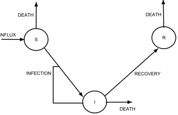
3.2 A Susceptible-Infectious-Recovered epidemics model. . . 38

3.3 A prey-predator model. . . 40

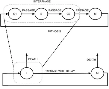
3.4 The cell cycle: interphase and mitotic phase. . . 41

3.5 A complete model of the cell cycle. . . 42

3.6 A model of the cell cycle with a delay. . . 43

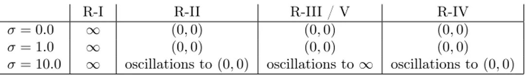
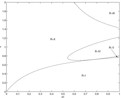
3.7 DDes tumor growth model and regions of behavior. . . 45

3.8 DDes numerical approximation (σ = 1) for the regions of Figure 3.7. . . 46

3.9 _{DDes numerical approximation (σ = 10) for the regions of Figure 3.7. . . .} 47

4.1 The semantics of the delay-as-duration approach. . . 52

4.2 _{Handling scheduled reactions in the DDa.} . . . 55

4.3 _{Events leading to the definition of the Dcme for the DDa. . . .} 57

4.4 _{DDa simulations (σ = 1) for the regions of Figure 3.7. . . .} 62

4.5 DDA simulations (σ = 10) for the regions of Figure 3.7. . . 63

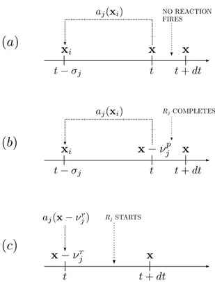
5.1 The semantics of the purely delayed approach. . . 66

5.2 _{Events leading to the definition of the Dcme for the PDa.} . . . 69

5.3 _{PDa simulations (σ = 1) for the regions of Figure 3.7. . . .} 72

5.4 PDa simulations (σ = 10) for the regions of Figure 3.7. . . 73

6.1 _{Maximum step size for a delayed reaction in the Dpf. . . .} 77

6.2 _{Events leading to the definition of the Dcme for the Dpf.} . . . 79

7.1 _{Over-scheduling in the PDa. . . .} 84

8.1 _{The LTSs for the two non bisimilar CCS processes. . . .} 99

8.2 _{The LTS for the CCS 2-reactions model. . . 101}

8.3 _{The LTS for the CCSd 2-reactions model. . . 107}

8.4 _{The LTS for the CCSp 2-reactions model. . . 117}

9.1 _{The LTS for the Bio-PEPA toy example. . . 125}

9.2 _{Timing aspects in Bio-PEPAd. . . 135}

(8)

(9)

List of Algorithms

1 _{SSa (t}0, x0, T ) . . . 27 2 _{DSSa DDa(t}0, x0, T ) . . . 56 3 _{DSSa PDa(t}0, x0, T ) . . . 68 4 _{DSSa Dpf (t}0, x0, T , H) . . . 78 5 _{DSSa mPDa (t}0, x0, T ) . . . 91 6 Full DSSa(t0, x0, T ) . . . 94

List of Acronyms

SSa Stochastic Simulation Algorithm DSSa Delay Stochastic Simulation Algorithm

DDa Delay-as-Duration Approach PDa Purely Delayed Approach

mPDa Purely Delayed Approach with Markings Dpf Delayed Propensity Functions

Full DSSa Full Delay Stochastic Simulation Algorithm ODe Ordinary Differential Equation

DDe Delay Differential Equation Cme Chemical Master Equation Dcme Delay Chemical Master Equation Ctmc Continuous-Time Markov Chain Gsmp Generalized Semi-Markov Process

LTS Labelled Transition System SOS Structural Operational Semantics

ST Starting-Terminating

CCS Calculus of Concurrent Systems

CCSp Calculus of Concurrent Systems with Delay-as-Duration Approach CCSd Calculus of Concurrent Systems with Purely Delayed Approach Bio-PEPA Bio-PEPA

(10)

(11)

Chapter 1

Introduction

In this chapter we provide motivations for this thesis. We start contextualizing this work in the interdisciplinary field of research named Systems Biology. We then briefly describe the contribution to the field and the structure of the thesis.

1.1 Motivations

Systems Biology in brief. Biochemistry, often conveniently described as the study of the chemistry of life, is a multifaceted science that includes the study of all forms of life and that utilizes basic concepts derived from Biology, Chemistry, Physics and Mathematics to achieve its goals. Biochemical research, which arose in the last century with the isolation and chemical characterization of organic compounds occurring in nature, is today an integral component of most modern biological research.

Most biological phenomena of concern to biochemists occur within small, living cells. In addi-tion to understanding the chemical structure and funcaddi-tion of the biomolecules that can be found in cells, it is equally important to comprehend the organizational structure and function of the membrane-limited aqueous environments called cells. Attempts to do the latter are now more common than in previous decades. Where biochemical processes take place in a cell and how these systems function in a coordinated manner are vital aspects of life that cannot be ignored in a meaningful study of biochemistry. Cell biology, the study of the morphological and functional organization of cells, is now an established field in biochemical research.

Computer Science and Mathematics can help the research in cell biology in several ways. For instance, it can provide biologists with models and formalisms able to describe and analyze complex systems such as cells. This rather new interdisciplinary field of research is named Systems Biology (Kitano, 2001; Ideker et al., 2001; Sauer et al., 2007).

Modeling biological systems. The approach which is used to solve a problem of system biology is typically the following: firstly the biological system has to be identified in all of its components, if possible. In particular all the involved elements and the interesting events have to be identified; this is generally one of the major problems because information may be lacking since some natural phenomena can not be properly observed. This results in a partial knowledge of the biological system itself. Such considerations are completely general and independent on the level of abstrac-tion of the target systems, indeed this applies when we refer to molecules and reacabstrac-tions, or to individuals and events within a population. The general spectrum of systems biology is wide and consider biological systems at any level of abstraction.

Whenever the system has been identified, it is possible to build models solely deterministic, stochastic, or even combinations of both. Models are built on the data which has been carried out by observing real natural systems.

(12)

2 CHAPTER 1. INTRODUCTION

Figure 1.1: The modeling schema in Systems Biology.

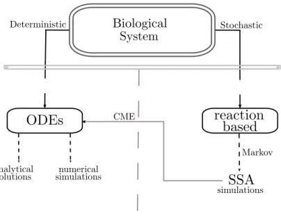
A deterministic model is generally a system of continuous differential equations which models the variation of concentrations of the involved components and whose terms are the modeling of the observed events. In the simplest case equations are Ordinary Differential Equations (ODes), and only in a few cases can be solved analytically finding the solution of the equation, the equi-libria and the bifurcation points. However, numerical simulations are always possible. Results obtained analyzing these models are satisfactory when modeling systems involving a huge number of components. Differently, when the size of the biological systems is small, deterministic models may not show some dynamics which are instead observed in real systems. This is caused by the fact that differential equations represent discrete quantities with continuous variables, and when quantities are close to zero this may become a too imprecise approximation. To overcome this incompleteness, stochastic models can be defined.

A stochastic model can be defined via the same principles used to derive a deterministic one. Typically, such a model is specified in a reaction-style notation. Such a model can potentially exhibit behaviors not captured by the deterministic counterpart since the involved quantities vary discretely and stochastically. Mathematically, such models are typically stochastic processes which, in most cases, are Markov since this permits easier analysis. To analyze Markov models Stochas-tic Simulation Algorithms (SSas) (Gillespie, 1976) have been defined to compute a single time evolution of the modeled system. One of the most interesting features of these algorithms is the introduction of the notion of propensity function for a reaction. Such functions are used to compute the probability of reactions to happen in a medium, once molecules are randomly distributed in space. The input of these algorithms are systems described as a set of reactions (i.e. rewriting rules) and an initial state. The time evolution is given by the probabilistic sequence of firing of the reactions in the system state. Such algorithms are logically related to deterministic systems via Chemical Master Equations (Cmes) (Gillespie, 1976) associated to simulated systems, these equations describes the time evolution of the probability of the system to occupy each one of a discrete set of states.

In Figure 1.1 the modeling schema we refer to is represented.

The use of delays. As we said, a crucial problem in modeling real systems is the identification of the components and events involved. Here difficulties come from the inherent experimental approach to this science. Delays can appear in a biological system at any level of abstraction. We go through this consideration by informally discussing two very simple scenarios. Firstly, let

(13)

1.1. MOTIVATIONS 3

Figure 1.2: The modeling schema extended with delays.

us consider a complex dynamics (macro-event) decomposed in a series of sequential sub-events (micro-events): to explicitly model such dynamics we must have full quantitative information about all the sequential sub-events. This requirement implies that, if some information is missing then a full model cannot be described, and this is quite a common scenario in real modeling. If this is the case, we can think about a raw abstraction of this system by considering, instead of the micro-events, the single-step macro-event, assuming that we have enough information for it to be modeled. Delays come into play at this stage when the average time for completion of the macro-event is known. Indeed, such an information can be used to have a more precise model, as we shall see in the rest of the thesis. Of course even though this is an abstraction of the exact model of the micro-events, this turns out to be the best that we can do in some situations. As we said, there is another scenario in which delays turn out to be useful. Namely, when a system is too complex to analyze, then using a similar assumption to above, we can replace a collection of micro-events by a model with delay at the macro-event level. In this case, the delay is used as a model-reduction technique which makes the model smaller, and the analysis potentially feasible. Models with delays. Deterministic modeling of biological systems with delays is mainly based on Delay Differential Equations (DDes) obtained by generalizing ODes. These equations are generally harder than ODes to be analyzed. Also, as for ODes the analysis of DDes can become imprecise due to the approximation introduced by representing discrete quantities by continuous variables when quantities are close to zero. Thus techniques for performing stochastic analysis of systems with delays have also been developed. Stochastic models with delays result in non-Markovian stochastic processes. Starting from the SSas for some of such processes Delay Stochastic Simulation Algorithms (DSSas) have been defined (Bratsun et al., 2005; Barrio et al., 2006; Barbuti et al., 2009b). In these cases such DSSas are logically related to deterministic systems via some Delayed Chemical Master Equation (Dcmes) (Barrio et al., 2006), an extension with delays of the Cmes.

In Figure 1.2 is represented the modeling schema extended with delays.

Formalisms from Computer Science. Experimental studies in biology have been producing a lot of data in the last years through enhanced techniques for analyzing biological systems; this increased in size and complexity existing models. Consequently, new methods supporting

(14)

devel-4 CHAPTER 1. INTRODUCTION

opment of complex models are required. Over the past decade Computer Science has been helpful in defining formalisms to describe complex systems. Concurrent systems theory is at the basis of most of the formalisms applied in systems biology.

There exist many formal languages, either based on process algebras, term–rewriting systems or different mathematical structures, worth noting: the Calculus of Concurrent Systems (CCS) (Milner, 1980), the π-calculus (Milner et al., 1992; Regev et al., 2001; Palamidessi, 2003) with its stochastic (Priami, 1995; Cardelli et al., 2009) and continuous (Kwiatkowski & Stark, 2008) variants, Beta binders (Priami & Quaglia, 2005; Guerriero et al., 2007), BlenX (Dematté et al., 2008), Bioambients (Regev et al., 2001), Brane calculi (Cardelli, 2005), PEPA (Hillston, 1996; Calder et al., 2006), Bio-PEPA (Ciocchetta & Hillston, 2009; Ciocchetta & Hillston, 2008; Akman et al., 2009), Petri Nets (Murata, 1989; Reddy et al., 1993) and some of their variants (Jensen, 1992; Leea et al., 2006), LBS (Pedersen & Plotkin, 2010), κ (Danos et al., 2009a; Danos et al., 2009b), the Calculus of Looping Sequences (Milazzo, 2007; Barbuti et al., 2008a; Barbuti et al., 2008b) and Bigraphs (Damgaard et al., 2008a; Damgaard et al., 2008b; Krivine et al., 2008). Some of these formalisms such as CCS, the π-calculus or PEPA have been defined to model different concurrent systems; however, subsequently they have been successfully applied in Systems Biology. As often happens, this motivated in defining ad-hoc languages such as BlenX, Bio-PEPA or κ. Also, biology inspired new models of computations so, for instance, DNA computing (Păun et al., 1998) or P-Systems (Păun, 2002) have been defined to compute by using cells or other types of molecules. In particular, the connection between P-Systems and process algebras has been actively studied (Cardelli & Păun, 2006; Barbuti et al., 2008c; Barbuti et al., 2008d; Barbuti et al., 2010c; Barbuti et al., 2010d).

A desired feature of a formalism is being compositional. A formal system is compositional if the semantics of composite object can be determined from the semantics of the components. Compositional systems therefore can be analyzed in a modular way, non compositional systems must be analyzed in their whole. Differential equations are not compositional since the solution of a set of equations can not be determined as a combination of the individual solutions of the equations. Differently, process algebras are typically compositional because of the semantics of their cooperation operators. In this approach chemical reacting entities are described by processes and biological reactions are modeled as cooperation/synchronization between processes, the act of synchronizing of communicating processes is interpreted as the firing of a reaction. In this thesis, for all the reasons we outlined we concentrate on process algebras when considering formal languages. However, all the theories we develop in the context of process algebras could be equivalently defined in different contexts (i.e. rewriting systems).

1.2 Contributions

In this thesis we address two major issues: firstly stochastic simulation and secondly formal mod-eling of biological systems with delays.

In the first part of the thesis we focus on DSSas. We analyze a well-known algorithm (Barrio et al., 2006) and its interpretation of delays, which is named delay-as-durations (DDa). We argue that such an algorithm is not suitable to simulate systems in which species involved in a delayed interaction can be involved at the same time in other interactions. Then we define a novel DSSa based on an pure interpretation of delays (PDa) which behaves more properly, even in its naïve definition, in simulating such systems. We provide both experimental evidences of the difference between the DDa and the PDa and we analyze mathematical foundations of both the algorithms. The PDa is then improved to avoid some inaccurate behaviors which may happen in its naïve definition. This new PDa, named PDa with markings, is then combined with the DDa.

Both these algorithms are based on the idea of delays as a scheduling policy, where the policy depends on the delays interpretation. For the sake of investigating further interpretations of delays we define a DDes-inspired DSSa where delays represent dependancies on past states of the simulated system. Investigating the mathematical foundations of this algorithm we prove it to be equivalent to the PDa.

(15)

1.3. RELATED WORK 5

This concludes the first part in which we rigorously present five algorithms for simulating stochastic systems with delays, and we prove relations among them. In the second part of the thesis we address the problem of supporting actions with delays in formal languages. To this extent, we provide two major results.

The former regards extending CCS to support non-instantaneous actions. More precisely, we define two extensions of CCS where actions follow either the delay-as-duration (CCSd) or the purely delayed approach (CCSp). Both the languages are conservative extensions of CCS, in the sense that the syntax of CCS processes is retained. Both languages are able to describe processes in which non-instantaneous actions are started and not completed. This introduces, in the case of CCSp, notions of competing actions internal to processes. For both the languages we define a Structural Operational Semantics (SOS) (Plotkin, 1981; Plotkin, 2004) in the Starting-Terminating (ST) style (van Glabbeek & Vaandrager, 1987; Bravetti et al., 1998) and bisimulation relations (Milner, 1980; Park, 1981). We discuss the effect of non-instantaneous actions on classical CCS operators, and we prove bisimulations to be congruences in both CCSd and CCSp.

The latter result of the second part concerns the enrichment of the stochastic process alge-bra Bio-PEPA with the possibility of assigning delays to actions following the delay-as-duration approach, yielding a new non-Markovian stochastic process algebra: Bio-PEPAd. Bio-PEPAd processes are defined with the original syntax of Bio-PEPA. We define notions similar to the one introduced for CCSd, namely process configurations, we define systems and a SOS in the ST-style for Bio-PEPAd. We formally define the encoding of Bio-PEPAd models in Generalized semi-Markov Processes (Gsmps), a class of non-semi-Markov processes, in input for the DDa and in sets of DDes. We prove results stating the relation between Bio-PEPA and Bio-PEPAd models.

1.3 Related Work

Stochastic simulation of non-delayed systems is mostly done by the SSa (Gillespie, 1976; Gillespie, 1977) and other SSa-based algorithms. Such an algorithm became more used in the last decade, whereas it has been defined in late 70’s. The theory of stochastic simulation of delayed system is, instead, a much newer research topic.

One of the first works on DSSas is (Barrio et al., 2006). In there, possibly different algorithms are informally discussed. For the informally discussed algorithms no clear mathematical founda-tions are investigated. For a specific variant of this algorithm more considerafounda-tions are given, even though correctness of that algorithm is not discussed. Such a variant is based on the interpretation of delays which in (Barbuti et al., 2009b) has been termed to be the delay-as-durations approach. Nowadays that algorithm, hereby named DDa, represents the most used simulation algorithm for systems with delays. In (Roussel & Zhu, 2006; Leier et al., 2007) the DDa is successfully applied to the simulation of a model of gene transcription and translation; we discuss those kind of models in Chapter 3. The DDa is based on the idea of scheduling reactions once that the reactants consumed by the reaction firing have been removed by the simulation state. As for all the scheduling-based algorithm, policies for handling scheduled reactions are defined based on rejection of generated random numbers. Such policies perform state-changes when scheduled reactions are handled. Summarizing, in this algorithm for each reaction two detached state-changes are induced. In (Barrio et al., 2006) a Dcme is presented and claimed to be the one related to systems simulated by the DDa. However, accordingly to our results, such a Dcme is not related to such systems since it refers to systems in which a single state-change is induced by a single reaction. We discuss this algorithm and our results in Chapter 4 and in Chapter 5.

Systems where is correct to think about a unique state-change induced by a reaction are those simulated by the algorithm introduced in (Bratsun et al., 2005). Such an algorithm is the first which implicitly adopted the approach we discuss in Chapter 5. However, mathematical foundations of the the algorithm presented in (Bratsun et al., 2005) are not investigated. We present an algorithm based on a purely delayed approach in the use of delays in Chapter 5 and for that algorithm we discuss its mathematical foundations.

(16)

2007) complex data structures are used so that rejection of generated random numbers is avoided. Moreover, mathematical foundations of the algorithms presented in (Cai, 2007) are studied and the correctness of the algorithm is discussed. Such a new algorithm is harder to be coded than the original DDa, but it is more time-efficient in practical usage. Similar results are obtained in (Anderson, 2007) where the algorithm presented in (Cai, 2007) is further improved by removing the complex data structures introduced to decrease the number of rejected random values. In (Zhou et al., 2008) these DSSas are analyzed by means of the moment probability functions instead, as in their corresponding works, by means of the probability density functions.

In (Anderson, 2007) for the first time is recognized a connection between some of the DSSas and a class of underlying non-Markovian stochastic processes. Moreover, in (Schlicht & Winkler, 2008) a a constructive proof of the existence of the non-Markovian stochastic process and a derivation of the involved probabilities is given. In (Jansen, 1995; Anderson, 2007; Shahrezaei et al., 2008) are also studied generalized SSa-based algorithms with time-dependent propensity functions. For the sake of studying DSSAs a result presented in (Shahrezaei et al., 2008) is recalled in Chapter 2.

The DSSas we discussed up to now are exact. Sometimes when thinking about DSSas it is convenient to decrease the precision of the algorithm and improve simulation performances. In this sense, a similar work has been done in non-delayed systems by proposing approximations of exact SSas (Gillespie, 2001; Rathinam et al., 2003; Cao et al., 2005). In (Tian et al., 2007) approximations are obtained by describing DDa-based systems by means of differential equations embedding stochastic and delayed effects. Such kind of equations find their conceptual base either in the Fokker-Planck or in the Langevin equations, as it happens for those presented in (Cao et al., 2005).

More complex form of delays have been studied for instance in (Marquez-Lago et al., 2010; Zhu et al., 2007; Ribeiro et al., 2009). In (Marquez-Lago et al., 2010) such a work spatial information of systems are introduced by means of ad-hoc probability distributed time delays. Such distributions are obtained by specialized experiments on the target system and then used in combination with the DSSas of (Barrio et al., 2006). Differently, in (Zhu et al., 2007; Ribeiro et al., 2009) reactions with multiple delays are considered.

As far as formal methods is concerned, process algebras has been studied in a lot of different formats: some including time, some including stochastic features and some combining both these aspects. So, for instance, process algebras with discrete or continuous notions of time has been defined (Moller & Tofts, 1990; Baeten & Bergstra, 1991; Nicollin & Sifakis, 1994; Hennessy & Regan, 1995) so that quantitative timing aspects can be investigated. In the context of Systems Biology, we are required to have a continuous-time domain underlying our systems.

In some semantics the notion of time is explicit, in the sense that a state of a system is given by some process and a global clock. The system can perform transitions modeling some changes in either the state process, once actions are performed, or in the global clock, by consuming time. In other cases, it is convenient to describe passage of time relative to previous actions. In the first case time is absolute (Corradini, 2000), whereas in the second is relative (Baeten & Bergstra, 1991). In (Baeten & Bergstra, 1997) the combinations of both the approaches is discussed, yielding to a notion of parametric timing. In most of these algebras explicit operators to spend time are required.

There are cases in which the notion of time is substituted by other features such as stochastic aspects of actions (Priami, 1995; Bravetti & Gorrieri, 2002; Ciocchetta & Hillston, 2009). In some stochastic process algebras it turns out that actions have no duration, making them instantaneous (Priami, 1995; Ciocchetta & Hillston, 2009). In this case, state transitions model instants between two distinct actions. If timing aspects of actions are ruled by special probability distributions then they can be abstracted from the mathematical structure underlying the algebras. In this case, the global clock can be retrieved by the frequency at which actions are performed, by means of the stochastic distributions ruling actions. Actually, this kind of languages are the most used in Systems Biology since their underlying mathematical structure is particularly convenient to perform model analysis. For the sake of our purposes most of these concepts are recalled in Chapter 2.

When actions have a duration or when delay is possible, classical operators of algebras such as the choice operator, may be affected in their original interpretation (Milner, 1980). This required

(17)

1.4. STRUCTURE OF THE THESIS 7

authors to define notions of choice as in (Baeten & Bergstra, 1991; Nicollin & Sifakis, 1994). When stochastic aspects are considered together with durations as in (Bravetti & Gorrieri, 2002), the resulting mathematical structure is of particular interest for modeling systems with delays, as we argue in Chapter 2.

In (Bravetti & Gorrieri, 2002) no explicit notion of time is present in the semantics, and hence no notion of quantitative duration is possible. This is a compromise between giving semantics without explicit notion of time and modeling durational actions. One of the best thing that we can do in this case is to simply characterize an action as a sequence of detached initiation and completion. In this sense, even if we are not able to precisely model a duration in a timed-framework, we are able to recognize a non-instantaneous event in our systems. This is the approach we generally adopt and, as in (Bravetti et al., 1998; Bravetti & Gorrieri, 2002), we use the Starting-Terminating (ST) style (van Glabbeek & Vaandrager, 1987; Hennessy, 1988; van Glabbeek, 1990) of non-timed semantics which turns out to be suitable to model systems with non-instantaneous actions. A similar work has been done in (Barbuti et al., 2010b; Barbuti et al., 2011b) where a variant of the CCS process algebra is extended to allow multiscale models of biological systems, namely models in which actions can happen at a different level of abstraction requiring different time scales.

We remark that we decided to use process algebras as the class of target formal methods since their compositional properties are desirable in modeling complex systems. However, other types of formal languages could have been used. Among all, it is worth citing Timed Automata based on finitely many real-valued clocks (Alur & Dill, 1994) and Timed Petri Nets (Reisig, 1985). These languages have been enriched with features for modeling real-time systems such as probability and stochasticity. In particular Stochastic Petri Nets (Marsan, 1989), Probabilistic Timed Petri Nets (Escalante & Dimopoulos, 1994), Probabilistic Timed Automata (Alur et al., 1992) and Stochastic Timed Automata (Cassandras & Lafortune, 2007) have been defined. It is common to use basic Petri Nets to qualitatively model chemical reacting systems without delays. In this case, to each places in the net a species is associated, and each token in a place corresponds to a molecule of the corresponding species. Transitions moving tokens from a place to another correspond to reactions.

When modeling biological systems with delays, more complex variants of basic nets such as Interval Timed Colored Petri Nets (van der Aalst, 1993) may be considered. In such nets time-stamps are attached to tokens to indicate the time in which they become available, in this sense this provides a way to track the time since a token is in the system. Such a mechanism of marking tokens is of inspiration for one of the algorithms we discuss in Chapter 7. Finally, there exist Petri Nets models with fixed delays or stochastic delays such as those in (Ramchandani, 1973; Sifakis, 1977; Zuberek, 1980).

1.4 Structure of the Thesis

The thesis is structured as follows.

- In Chapter 2 we recall some background notions of probability theory, stochastic processes, differential equations, stochastic simulation of biological systems and formal languages as-sumed in the rest of the thesis. Particular detail is used to introduce important results such as the relation between the Stochastic Simulation Algorithm and its associated Chemical Master Equation.

- In Chapter 3 we discuss some target biological systems with delays. We concentrate on some basic cellular models, epidemics models and evolutionary models and we define them in both a deterministic and a stochastic fashion. For all of those, we discuss role of delays in their modeling. Finally, we present a model of the cell cycle with a delay used as a running example along the thesis. Deterministic simulations of such a model are discussed.

For the sake of clarity, the thesis is divided in two major parts, where the first is functional to the definition of the second. In the first part, from Chapter 4 to 7, Delay Stochastic Simulation Algorithms are presented.

(18)

- In Chapter 4 a well-known algorithm based on a notion of “delays as durations” approach (DDa), is presented. Such an algorithm is based on a scheduling policy preventing that species involved in a delayed interaction can be involved at the same time in other interactions. We discuss the mathematical foundations of the DDa by defining a Delay Chemical Master Equation (Dcme) and we prove the correctness of the DDa. We then apply the algorithm to the simulation of the cell cycle model presented in Chapter 3, and we compare results of the deterministic and stochastic simulations.

- In Chapter 5 we present a novel algorithm based on a “purely delayed” interpretation (PDa) of delays. Such an algorithm is defined so that species involved in a delayed interaction can be involved at the same time in other interactions. We apply a naïve definition of the algorithm to the simulation of the cell cycle model, and we compare results of all the simulations performed. Results suggest that this new approach is a better candidate than the DDa for such type of systems. We then investigate the mathematical foundation of the PDa. We prove the algorithm to be correct and we define a Dcme for systems simulated by such an algorithm. As expected, such a Dcme differs from the one of the DDa.

- In Chapter 6 we present a novel history-dependent algorithm (Dpf). Such an algorithm is inspired in its definition by deterministic models with delays, hence delays are used to define dependancies on the past-states of the system. As for the other algorithms we analyze its mathematical foundations. We prove this algorithm to be correct, and we show that target systems of the Dpf underly the same Dcme of PDa systems, leading to the equivalence of the two algorithms.

- In Chapter 7 we improve the naïve PDa presented in Chapter 5 by means of a notion of marking of the molecules in the system state, yielding to the definition of a new algorithm, the mPDa. We then combine this new algorithm with the DDa introduced in Chapter 4, yielding to the definition of a new algorithm able to correctly simulate systems in which for some reactions the species involved in a delayed interaction can not be involved at the same time in other interactions, whereas others can.

In the second part, we discuss formal modeling biological systems with delays.

- In Chapter 8 we extend the Calculus of Concurrent Systems (CCS) with non-instantaneous actions. More precisely, we define two extensions of CCS where actions follow either the delay-as-duration (CCSd) or the purely delayed approach (CCSp). Both the languages assume the same syntax of CCS processes, and for both we define a notion of process configuration necessary to have processes in which non-instantaneous actions are started and not completed. For both the languages we define a labeled semantics and bisimulation relations. We discuss the effect of non-instantaneous actions on classical CCS operators, and we prove bisimulations to be congruences even in the case of non-instantaneous actions. - In Chapter 9 we enrich the stochastic process algebra Bio-PEPA with the possibility

of assigning delays to actions following the delay-as-duration approach, yielding a new non-Markovian stochastic process algebra: Bio-PEPAd. Bio-PEPAd processes are defined with the original syntax of Bio-PEPA. We define process configurations, systems and we define a labeled semantics for Bio-PEPAd. We formally define the encoding of Bio-PEPAd models in Generalized semi-Markov Processes in input for the DDa and in sets of differential equa-tions with delays. Also, we investigate the relation between Bio-PEPA and Bio-PEPAd models.

Finally, we give some conclusions and discuss further work in Chapter 10.

1.5 Published Material

Part of the material presented in this thesis has appeared in some publications or has been sub-mitted for publication, in particular:

(19)

1.5. PUBLISHED MATERIAL 9

- The algorithm with delay-as-duration approach of Section 4.2, the one with purely delayed approach of Section 5.2, the stochastic and deterministic simulations of the cell cycle model of Sections 3.2, 4.4, and 5.4 appear in (Barbuti et al., 2009b).

- The algorithm with delayed propensity functions presented in Section 6.2, and its compar-ison with the PDa of Section 6.3 appears in (Barbuti et al., 2011b).

- The definition of the purely delayed approach with markings of Section 7.2 and its combi-nation with the delay-as-duration approach of Section 7.3 appear in (Barbuti et al., 2011a). - The definition of Bio-PEPAd of Sections 9.2.1, 9.2.2 and 9.4.1 initially appeared in (Caravagna & Hillston, 2010). _{Moreover, an extended version including Sections 9.2.3} and 9.3 appears in (Caravagna & Hillston, 2011).

All the published material is presented in this thesis in revised and extended form.

Extra material. Most of the models and the simulation software used to produce results outlined in this thesis, as well as the publications cited in the previous section, can be found at the web page of the “Research Group on Modelling, Simulation and Verification of Biological Systems" of the Department of Computer Science at the University of Pisa

http://www.di.unipi.it/msvbio/ or requested directly from the author at caravagn@di.unipi.it.

(20)

(21)

Chapter 2

Background

Since Systems Biology is an interdisciplinary field of research involving mathematics, biology and computer science at different level of detail, giving a comprehensive background of the required notions is a non trivial task. In this chapter we try to recall most of the background necessary to understand the results outlined in this thesis. Of course, this thesis is neither pure mathematics nor biology, so those parts are presented at a more introductory level. Moreover, the biological knowledge we need is recalled only when presenting models of target systems in Chapter 3. In the next, we assume the reader to be familiar with basic notions of calculus, which is something we need to discuss the mathematical foundations of the algorithms we present.

We start introducing notions of probability theory, random variables and some well-known probability distributions. We briefly introduce stochastic processes in their most common form, namely Markov processes, and a class of non-Markov processes useful to understand systems with non-instantaneous actions.

As far as deterministic models are concerned, we introduce differential equations both in delayed and non-delayed form. We introduce with a bit more detail stochastic models and an algorithm for simulating their time-evolution. We provide arguments about the mathematical foundations of such an algorithm and one of its generalization, as they are of help to discuss more complex results we present in the first part of the thesis.

As far as formal models are concerned, we recall basic notions to give a mathematical meaning to our languages and to the models we discuss. We introduce also techniques to define such mathematical objects for the languages we define in the second part of the thesis.

For all the concepts we recall, we discuss via simple examples their usability for our purposes.

2.1 Notions of Probability theory

In this section we recall some concepts from probability theory used along the thesis. Intuitively, probability is a way of measuring knowledge that an event will occur or has occurred. In probability theory, the “probability of E", hereby denoted P(E), is defined so that P satisfies the Kolmogorov axioms. More precisely, a triple (Ω, F, P) is a measure space once that for any E ∈ F it holds that P(E) > 0, moreover P(Ω) = 1 and, for any sequence of pairwise disjoint events E1, E2, . . ., En, it

holds P(E1∪ . . . ∪ En) =P n

i=1P(Ei). So (Ω, F, P) is a probability space, with sample space Ω, event

space F and probability measure P. For the sake of our purposes, we introduce discrete random variables with N as sample space and continuous random variables with R as sample space.

If X is a discrete random variable there exist a probability mass function f characterizing the distribution of X and such that for any x ∈ N it holds f (x) ≥ 0 andP

Nf (i) = 1. The probability

(22)

12 CHAPTER 2. BACKGROUND

cumulative distribution function F : N → [0, 1] such that P(X ≤ x) = F (x) =

X

y≤x

f (x) . (2.1)

Similarly, if X is a continuous random variable there exist a probability density function f charac-terizing the distribution of X and such that for any x ∈ R it holds f (x) ≥ 0 andR

Rf (x)dx = 1.

The probability of X having values in the closed real-valued interval [a, b] is

P(a ≤ X ≤ b) = Z b

a

f (x)dx .

In general, the probability of X being smaller than x is defined by the cumulative distribution function F : R → [0, 1]

P(X ≤ x) = F (x) = Z x

−∞

f (u)du . (2.2)

The cumulative distribution function F satisfies two intuitive equations lim

x→−∞F (x) = 0 x→+∞lim F (x) = 1 .

Moreover, F is a non-decreasing function and if X is continuous in x then F (x) is continuous, so we have that

∀b ∈ R. P(X = b) = F (b) − lim

x→b−F (x) = 0 (2.3)

since the left-limit of F evaluates as limx→b−F (x) = F (b). Finally, it is easy to notice that

P(X > x) = Z R f (u)du − Z x −∞f (u)du = 1 − P(X ≤ x) = 1 − F (x) . (2.4) Before introducing some special cases of random variables, we introduce the notion of condi-tioned probability: P(A | B) represents the condicondi-tioned probability of “A given B" and is defined as

P(A | B) = P(A; B) P(B)

(2.5) where A; B denotes the event “A and B" and P(B) 6= 0. Conditioned probability gives a way of measuring changes in the probability of an event A once we have some information about a related event B. When A and B are independent it holds that P(A; B) = P(A)P(B) and hence P(A | B) = P(A).

A simple equation on conditioned probability can be immediately stated: given events A, B and C we have

P(A | B; C)P(B | C) = P(A; B | C) (2.6)

which can be easily verified by the definition of conditioned probability since

P(A | B; C)P(B | C) = P(A; B; C) P(B; C) P(B; C) P(C) = P(A; B; C) P(C) = P(A; B | C) .

The uniform distribution. Intuitively, a continuous uniform distribution is a family of distri-butions defined by lower and upper bounds a and b, respectively, such that all intervals of the same length in [a, b] are equally probable. If X is uniformly distributed in [a, b] we write

(23)

2.1. NOTIONS OF PROBABILITY THEORY 13

If a = 0 and b = 1 the resulting distribution U [0, 1] is called a standard uniform distribution. Analytically, the density characterizing X ∼ U [a, b] is defined as

f (x) = (

(b − a)−1, a ≤ x ≤ b 0, x < a ∧ x > b while the cumulative distribution function is

F (x) =        0, x < a x − a b − a, a ≤ x ≤ b 1, x > b . A useful property of the standard uniform distribution is that

X ∼ U [0, 1] =⇒ (1 − X) ∼ U [0, 1] .

The exponential distribution. A widely used continuous distribution in the context of systems biology is the exponential distribution. If X has exponential distribution with parameter λ > 0 we write

X ∼ E xp (λ) and X has a probability density function

f (x) = (

λe−λx, x ≥ 0 0, x < 0 . The cumulative distribution function is given by

F (x) = ( 0, x < 0 1 − e−λx, x ≥ 0 since Z x 0 ue−λudu = 1 − e−λx.

The exponential distribution has infinite support, where the support of a distribution is the smallest closed interval whose complement has probability zero. Practically, this means that given any interval [a, b] the probability of generating an exponentially distributed value in such interval is non zero, namely if X ∼ E xp (λ) then

∀a, b ≥ 0. a < b =⇒ P(a ≤ X ≤ b) 6= 0 . (2.7) A very important property characterize solely this distribution: the memoryless property. If X ∼ E xp (λ) then for any positive s, t ∈ R

P(X > s + t | X > t) = P(X > s) (2.8) which holds since

P(X > s + t | X > t) = P (X > s + t; X > s)P (X > t)−1 = P (X > s + t)P (X > t)−1 = e−λ(s+t)eλt= e−λs.

Finally, let {Xi ∼ Exp (λi) | i = 1, . . . , n} where all the variables are independent, then let us

define the new variable Y = min{ X1, . . . , Xn}. For such a variable we have

P(Y > x) = P(X1> x; . . . ; Xn> x) = n Y i=1 P(Xi> x) = e−x Pn i=1λi

which means that

(24)

Sampling from the exponential distribution. We discuss now how to generate exponentially distributed numbers, an activity on which stochastic simulation is heavily based. The sampling of a value for a continuous random variable can be obtained by an Inverse Monte-Carlo Algorithm based on the following considerations: given a continuous random variable X with cumulative distribution F and given p ∼ U [0, 1] it holds that

x = F−1(p) . (2.9)

Despite of being generally hard the computation of F−1, for the exponential distribution we know how to evaluate the inverse of F . Let us assume X ∼ E xp (λ), we start by noting that by definition of the exponential distribution

P(X ≤ x) = Z x

0

λe−λudu

is the probability of X being smaller then x. Such value is a probability, so is a number in [0, 1]; let us assume that we can pick a number r ∼ U [0, 1]. We can write

Z x

0

λe−λudu = r which integrates as

e−λx= 1 − r

and, as we know from the property of the uniform distribution, if r ∼ U [0, 1] then (1 − r) ∼ U [0, 1]. Computing now the value for x is fairly easy since when applying the logarithm we have

x = λ−1ln r−1. (2.10)

This last equation permits us to generate a sample for X once that we can pick a value for r. The Erlang distribution. The exponential distribution is a special case of a more general continuous distribution, the Erlang distribution. A random variable X following such a distribution is denoted as

X ∼ Γ(n, λ)

where n ∈ N, n > 0 is called the shape, and λ > 0 is the rate. When n ∈ R this distribution is called the Gamma distribution. Erlang distribution has probability density function defined as

f (x) =    λnxn−1e−λx (n − 1)! , x ≥ 0 0, x < 0 .

and cumulative distribution function defined as F (x) =    0, x < 0 1 − e−λxPn−1 i=0 (λx)i i! , x ≥ 0 .

Three important properties can be stated for this distribution: firstly, when the shape is 1 it reduces to the exponential distribution

X ∼ Γ(1, λ) =⇒ X ∼ E xp (λ)

as it can be easily verified by the analytical form of the density function. Secondly, the summation of independent exponentially distributed random variables follows an Erlang distribution, namely

X1∼ Exp (λ) ∧ X2∼ Exp (λ) =⇒ (X1+ X2) ∼ Γ(2, λ) .

and we also have that

X1∼ Γ(n1, λ) ∧ X2∼ Γ(n2, λ) =⇒ (X1+ X2) ∼ Γ(n1+ n2, λ)

again if X1 and X2 are independent. Finally, it is easy to notice that this distribution has infinite

(25)

2.2. NOTIONS OF STOCHASTIC PROCESSES 15

2.2 Notions of Stochastic Processes

Here we recall some of the definitions of stochastic processes we use in the thesis, for a broad introduction to such a topic the reader can refer to (Ross, 1995). A stochastic process X = {X(t), t ∈ T } is a collection of random variables. Assuming T to represent time, if the set T is countable then the process is discrete-time, otherwise is continuous-time. Moreover, if X(t) assumes discrete values, then the process is discrete-state, otherwise is continuous-state. In the context of this thesis we consider continuous-time and discrete-state stochastic processes with T = R and X(t) assuming values on some discrete vector-space. In this sense, the discrete-state of the processes we consider represent exact numbers which, in our context of application, denote individuals in a system.

An important class of stochastic processes is the class of those satisfying the Markov property, namely the fact that given the present state of the process, its future is independent on the past. Not all the stochastic processes satisfy this property; in the next we introduce Continuous-Time Markov Chains (Ctmcs) which satisfy such a property and Generalized Semi-Markov Processes (GSMP) which do not satisfy the Markov property.

Continuous-Time Markov Chains. Let us consider a continuous-time stochastic process X = {X(t), t ∈ R} where the set of all possible values taken by X(t) is a discrete set (e.g. the vector-space Nn), we say that X is a Ctmc if for any integer k ≥ 0, sequence of time instants t0< t1<

· · · < tk and states x0, . . . , xk it satisfies the Markov property

P(X(tk) = xk| X(tk−1) = xk−1, . . . , X(t1) = x1) = P(X(tk) = xk | X(tk−1) = xk−1) . (2.11)

Intuitively, this means that given the system in state xk−1at time tk−1the probability of moving

to state xk at time tk depends only on the current state, and not on all the path starting in x1

at time t1 and ending up in the current state. Notice the similarity between the Markov Property

and the memoryless property of the exponential distribution. Indeed, the exponential distribution is the only continuous probability distribution which exhibits such a property, hence it is the only one used in the definition of Ctmcs.

Formally, a CTMC is defined as follows.

Definition (Continuous Time Markov Chain). A CTMC is a triple hS, R, πi, where • S is the finite set of states;

• R : S × S → R≥0 _{is the transition function;}

• π0: S × S → [0, 1] is the starting distribution.

The system is assumed to pass from a configuration modeled by a state x ∈ S to another one modeled by a state x0 ∈ S by consuming an exponentially distributed quantity of time

Exp (R(x, x0)) .

This means that, by using the properties about the minimum of exponentially distributed random variables, the sojourn time in state x is distributed according to

Exp X

x00_∈S

R(x, x00) !

where the summationP

x0_∈SR(x, x0) is called the exit rate of state x. Practically this means that,

when jumping between the states of the chain, all the outgoing transitions compete for being chosen forming a race condition, and the sojourn time in a state is driven by the quickest of its outgoing transitions. Whenever the sojourn time is established, among all the possible states reachable from x, the state x0 the system moves to is chosen according to the weighted probability

R(x, x0) P

x00_∈SR(x, x00)

(26)

Figure 2.1: The Ctmc for the linear birth-death process.

This last probability distributions is ruled by the Discrete-Time Markov Chain embedded in any Ctmc, this embedded chain contains probabilistic information about the resolution of the transi-tions to fire in a state and, being discrete, it does not contain information about the distribution of the sojourn times.

Finally, the system is assumed to start from a configuration modeled by a state x ∈ S with probability π0(x), andPx∈Sπ0(x) = 1. If the set of states of the CTMC is finite, S = {x1, . . . , xn},

then the transition function R can be represented as a square infinitesimal generator matrix π ∈ Rn×nsuch that

πi,j = R(xi, xj) πi,i= −

X

j6=i

R(xi, xj) .

Some Markov chains are said to be time-homogeneous when the probability of a transition satisfies P(X(tk+1) = x | X(tk) = y) = P(X(tk) = x | X(tk−1) = y) . (2.12)

Such chains satisfy a desirable property once they have finite state space: the transition matrix is the same after each step, so the k-th step transition probability is the k-th power of the transition matrix, πk=Qk

i=1π where we assume the classic matrix multiplication. In this sense, a stationary

distribution π is a row vector satisfying

π = ππ . (2.13)

Intuitively, the stationary distribution π is the fixed point of a linear transformation describing the equilibrium probability of the system, and under some conditions on π it is uniquely determined.

In order to clarify the use of Ctmcs in modeling, let us consider a single population assuming discrete values in {n ∈ N | n > 0}. In this population death and birth may happen, if the former happens population increases by one, conversely if the latter happens population decreases by one. We assume an infinite set of discrete states S = {xi | xi = i ∧ i ≥ 0}; the transition function is

such that

R(xi, xi+1) = λi R(xi, xi−1) = µi

and ∀i, j. R(xi, xj) = 0 if |i − j| > 1. This means that, for instance, when the system is in state xi

it waits a quantity of time distributed according to E xp (λi+ µi)

A graphical representation of this Ctmc for the linear birth-death process is given in Figure 2.1. The values {λi | i ≥ 0} and {µi | i ≥ 1} are called the birth and the death rates so when

there are i people in the system the time until the next birth is exponential with rate λi and is

independent of the time until the next death, which is exponential with rate µi.

Generalized Semi-Markov Processes. Using Markov processes is generally convenient since they are described by exponential functions which have a clear structure and are easy to understand. However, retrieving the Markov property for some systems may be hard or even unfeasible, in fact not all stochastic processes are Markov. Considering non-Markov processes is very hard since, in general, they are based on arbitrary distributions. However under some circumstances some considerations can be stated.

We introduce Generalized Semi-Markov Process (Gsmp) as in (Bravetti et al., 1998; Bravetti & Gorrieri, 2002), an extension of those originally defined in (Matthes, 1962). Such processes are

(27)

2.3. DETERMINISTIC MODELS OF BIOLOGICAL SYSTEMS 17

Figure 2.2: An example Gsmp.

discrete processes, where the embedded state process is a Markov chain, but the time between jumps is a random variable of arbitrary distribution, which may be dependent on the two states between which the move is made. If in each state there is a single jump event, then the process is a Semi-Markov Process, in contrast to a Gsmp which may have more than one event concurrently running in each state. If in a Semi-Markov process the times between jumps are exponentially distributed, namely jumps are memoryless, then it is a Ctmc. Gsmps have been used to give a stochastic process description of a large class of discrete-event simulations (Cox, 1955).

Informally a Gsmp is a process in which each state is characterized by a set of active elements, each with an associated lifetime. A state change occurs when an active element completes a lifetime and all interrupted elements record their residual lifetimes. Whenever the element is again active it resumes its remaining lifetime. If the lifetimes are exponential we may disregard the residual lifetimes, restarting each element with a new lifetime whenever it is active.

Definition (Generalized Semi-Markov Process) A Generalized Semi-Markov Process (Gsmp) is defined on a set of states {x | x ∈ X}. For each x there are active elements s, from the set S, which decay at the rate r(s, x), s ∈ S. When the active element s dies, the process moves to state x0 ∈ X with probability p(x, s, x0_).

Another consideration is worth discussing. Markov processes, semi-Markov processes and Gsmps differ for the set of instants of process life which satisfy the Markov property, namely those instants such that the future behavior of the stochastic process depends only on the current state of the process and not on its past behavior. For Markov Chains the Markov property holds in every instant of process life, for Semi-Markov Processes it holds only in the instants of state change and, for a Gsmp it never holds but can be retrieved through a different representation of process states. Such representation is given by turning each state into a continuous infinity of states by the standard technique discussed in (Cox, 1955).

We present now an example of Gsmps taken from (Bravetti & Gorrieri, 2002). Let us consider two activities a and b executed in parallel, both distributed with two arbitrary distributions. In Figure 2.2 the possible evolution of the two activities is given. In there, each state is labeled with the set of activities which are in execution during the period of time the system stays in the state. As expected, in the beginning both activities are together in execution and the system stays in the initial state until one activity or both contemporaneously terminates. When this happens the system performs the transition labeled with the terminated actions. If a terminates before b the system reaches the state labeled with b. In such a state the activity b continues its execution until it terminates. As a consequence the sojourn time of the system in the state labeled with b is given by the residual distribution of activity b, and is not determined simply by the fact that the system is in this state but depends on the time b has already spent in execution in the initial state. Clearly, this process is Markovian not even in the instant when this state is entered.

2.3 Deterministic Models of Biological Systems

Deterministic models of biological systems are the most used and widespread models of biological systems since the last century. In this section we introduce both the non-delayed and the delayed

(28)

deterministic frameworks for the modeling of biological systems. The former is characterized by Ordinary Differential Equations and the latter by Delay Differential Equations, a generalization of the ordinary ones.

2.3.1 Ordinary Differential Equations

A Differential Equation is an equation involving an unknown function and its derivatives; when the unknown function is a function of a single independent variable the equation is an Ordinary Differential Equation (ODe). There exist a variety of such equations, we concentrate on those useful in the context of our work. Typically, the models we consider are described as a set of ODes which describes the time-evolution of the concentrations of the involved species in a given volume. Assuming the state of the system to be represented as a n-dimensional real-valued vector, the general form of an ODe for X(t) ∈ Rn is

dX

dt = f (t, X(t)) (2.14)

where dX/dt may depend on the state of the system at time t, denoted as X(t), and not on any previous states. Notice that, differently from Ctmcs, in the context of systems biology the real-valued representation of X(t) is such that we do not represent exact numbers, but instead we represent concentrations.

Much study has been devoted to the solution of such equations; when the equation is linear, it can be solved by analytical methods. So for instance an equation of the form

dX

dt = λX (2.15)

has a well-known solution. Such an equation reads as “the variation in the size of X in the infinitesimal time dt is given by λX” and its analytical solution can be easily computed integrating the equation

dX X = λdt

and imposing the initial condition X(t0) = x0. This means that the solution of the equation is

X(t) = X(t0) exp (λt) (2.16)

where X(t0) represent the initial value for X at time t0. These kind of equations, which have

always an exponential solutions, are said to model the exponential decay/growth of X(t). In fact, once that the value for λ is known, if it is positive the solution models a growth, otherwise a decay. Unfortunately, most of the interesting differential equations used in modeling biological systems are non-linear and, with a few exceptions, cannot be solved exactly. Approximate solutions are obtained by well-known numerical simulation algorithms: Euler forward and backward methods and Runge-Kutta iterative methods, to name but a few. Of course, this kind of analysis gives in general less information than the one given by analytical solutions. For an introduction to the theory of ODes the reader is referred to (Agarwal & O’Regan, 2008).

In the context of biological systems ODes have been used to study notions of chemical kinetics by means of Reaction Rate Equations, which are briefly introduced in the forthcoming section. Chemical kinetics and Reaction Rate Equations

In this section we introduce some notions of chemical kinetics and we discuss how to define for some forms of chemical reactions their Reaction Rate Equations (RRes). For a broad introduction to the theory of chemical kinetics the reader is referred to (Segel, 1993).

Chemical kinetics is the theory which relates changes in the experimental conditions with the rate (or frequency) at which chemical reactions fire, also it relates such changes with the process of creating the results of the reaction. In order to fire a chemical reaction it is necessary that the

(29)

2.3. DETERMINISTIC MODELS OF BIOLOGICAL SYSTEMS 19

colliding reactants have a minimum level of activation energy and, if it is so, the firing of a reaction implies the break of the chemical bonds and the creation of new chemical bonds. These new chemical bonds, after some rearrangement processes leading to the creating of a stable chemical state, are such that the products of the reaction are present in the solution where the reaction fired.

Some of the main factors affecting the rate of a chemical reaction are the type and strength of the chemical bonds characterizing the reactants, the physical state of the medium, the quantity of the reactants and the average thermal energy of the system. As far as the quantity of the reactants is involved, the collision theory of chemical reactions states that the probability of a collision between reactants in a medium is proportional to their concentrations. Other quantities such as thermal energy of the molecules affect the rate as depicted by the Maxwell-Boltzmann equation.

The RRe for a chemical reaction is an ODe which links the reaction rate with some of the factors we discussed. Typically, the factors considered are concentrations of the reactants and constant coefficients. In order to define rate equations we assume a generic reaction of the form

l1R1+ . . . lnRn k

7−→ l0₁P1+ . . . + l0n0Pn0

transforming, for each reactant Ri with i = 1, . . . , n, a number li of molecules and producing, for

each product Pj with j = 1, . . . , n0, a number l0j of molecules. Notice that reactants and products

can be mathematically represented as multisets, namely sets with repetitions. In that case, we would say that element Ri belongs to the multiset of reactants with multiplicity li, and element

Pj belongs to the multiset of products with multiplicity l0j. When we want to denote an empty

multiset we use the symbol ∅.

The reaction is equipped with a kinetic constant k ∈ R, a parameter relating temperature and other characterizing quantities of the target solution. Typically, chemical reactions are distinct dependently on the number of reactants they have: when they have zero (n = 0), one (n = 1) or two (n = 2) reactants they are considered 0-order, 1-order or 2-order reactions, respectively. Reactions involving more than 2 reactants can often be represented as multi-step 2-order reactions. When the chemical kinetics is ruled by the law of mass action the reaction rate is proportional to the concentrations of the individual reactants involved. This definition assumes that the reaction happens in a homogeneous medium. Formally, such law states that the consumption and the production of the molecule involved in the reaction depends on the quantity

k

n

Y

i=1

[Ri]li

where [Ri] represents the concentration of molecules Ri in the solution. From this quantity, a set

of ODes describing the changes induced by such reaction can be defined as d[Ri] dt = −k n Y i=1 [Ri]li d[Pi] dt = k n Y i=1 [Ri]li (2.17)

Intuitively, we define an ODe for each species appearing in the reaction, namely for any reactant and product. All these ODes share a common term which is given by the law ruling the kinetics of the reaction. More precisely, this term is negative for the species involved as reactants, and is positive for those appearing as products and is both positive and negative for the combination of the cases.

As an example, let us consider two simple biochemical reactions 2A k1

7−−→B A + B k2

7−−→ C

transforming two molecules A into the single molecule B with kinetic constant k, and transforming one molecule A and one molecule B in a molecule C with kinetic constant k0. By the law of mass