A methodology for the generation of synthetic input data for hybrid microgrid simulations

i

POLITECNICO DI MILANO

School of Industrial and Information Engineering

Master of Science in

Energy Engineering

A methodology for the generation of synthetic

input data for hybrid microgrid simulations.

Advisor: Prof. Marco Astolfi

Co-Advisor: Dr. Simone Mazzola

Candidate:

Alessia Ferraris, identification number 837067

iii

Ringraziamenti

Un doveroso grazie al professor Marco Astolfi, per la sua disponibiltà e pazienza fin dal principio, per la sua franchezza e attenzione nel seguirmi. Ringrazio anche Simone per la gentilezza, per i consigli e l’aiuto datomi, ed Elena, per il supporto nella prima parte del lavoro.

Il più grande grazie va a mia mamma e mio papà, per avermi dato questa grande possibilità, per i sacrifici, per avermi sostenuta sempre in ogni situazione, vi voglio bene. Ringrazio Loris, per la pazienza infinita, per essere un porto sicuro durante ogni tempesta, per essere il mio migliore amico oltre al resto, per la condivisione di ogni traguardo raggiunto e che verrà.

Ringrazio le mie zie Manuela e Valeria, le mie cugine Michela e Martina, Matilde gioia del mio cuore, e tutti i membri della famiglia uno per uno. Grazie perchè essere sempre uniti, al di là delle cose materiali, è il vero significato della parola famiglia.

Ringrazio i miei amici, la mia seconda famiglia: Maggie, per ascoltarmi e capirmi in ogni situazione, per essere un punto fermo nella mia vita da tanti anni e per la certezza che sarà così per sempre; Erica per avermi insegnato il coraggio di inseguire il proprio sogno contro ogni difficioltà; Sofia per la sua spontaneità e indipendenza, per avermi mostrato l’importanza di essere sè stessi; Giulia per i preziosi consigli, perchè ci vediamo poco ma quando ci vediamo nulla è cambiato; le mie coinquiline, per aver condiviso parte di questa importante esperienza con me; ringrazio anche Marco, Bobo, Robi, Pietro, la Ro e tutti gli altri presenti e non, di certo non meno importanti, perchè gli anni passano ma la nostra amicizia non cambia mai.

Ringrazio Elisa e Annalisa, i miei leoni, che hanno condiviso questo percorso con me: solo voi potete capire fino in fondo le emozioni che abbiamo vissuto. Grazie per tutte le ore passate insieme. Le fatiche, condivise con voi, sembravano pesare meno e le risate valere di più. Sarete tra i ricordi più belli di questa esperienza.

Ringrazio infine i miei nonni Piera, Adriano e Caterina che se ne sono andati durante questo percorso. Grazie per aver sempre creduto in me senza riserve, per l’orgoglio che vi riempiva il petto nel parlare dei miei traguardi e per aver saputo alleggerire i miei momenti di delusione con le giuste parole di conforto.

A voi dedico questo lavoro.

“I nonni ti vedono crescere, sapendo che ti lasceranno prima degli altri. Forse é per questo che ti amano piú di tutti.”

i

Index

1. Introduction ... 1

1.1. Access to electricity in isolated contexts ... 1

1.2. Electrification: statistical data and global situation ... 2

1.3. Developing countries VS developed contexts electrification ... 5

1.4. Rural electrification: off-grid VS grid-connected systems ... 7

1.5. Renewable sources integration ... 7

2. Design of a rural microgrid ... 9

2.1. Main targets of a microgrid ... 9

2.2. Design of a microgrid: phases ... 10

2.3. Design methods ... 11

2.4. Input data: renewable sources and load demand ... 13

2.5. Objective: annual profiles reconstruction from latitude and longitude coordinates ... 14

3. Renewable sources ... 17

3.1. Renewable generators ... 17

3.2. Solar radiation ... 19

3.2.1. Typical meteorological year’ (TMY) profile ... 21

3.2.2. Synthetic data generation ... 21

3.2.3. Literature review ... 22

3.2.4. Proposed method ... 26

3.2.5. From GTI to power ... 41

3.3. Wind energy... 43

3.3.1. Wind energy: ‘Typical meteorological year’ (TMY) profile ... 44

3.3.2. Wind energy: synthetic data generation ... 45

3.3.3. Literature models scenario ... 45

3.3.4. Proposed method ... 46

3.3.5. From wind speed to power ... 58

4. Load characterization ... 69

ii

4.2. Agriculture and productive needs ... 70

4.2.1. Irrigation and water needs ... 70

4.2.2. Irrigation energy demand: methodology proposed. ... 71

4.2.3. Domestic and potable water needs ... 77

4.2.4. Productive needs and biomass availability ... 81

4.2.5. Dataset used ... 86

4.3. Basic needs ... 87

4.4. Annual load profile reconstruction ... 90

4.4.1. Mathematical formulation ... 90

4.4.2. LoadProGen: Matlab implementation ... 94

Conclusions ... 99

iii

List of figures

Figure 1.1 - World access to electricity (% of population with the access) [6]. ... 3

Figure 1.2 - Electrification rate in 16 big Indian states from 1970to 2000. ... 4

Figure 1.3 - Distribution of population without access to electricity in African regions [9]. ... 5

Figure 1.4 - The 10 reviewed microgrids [10]. ... 6

Figure 1.5 - Global heat map of renewable microgrids progress [13]. ... 8

Figure 2.1 - Microgrid’s layout. ... 9

Figure 2.2 - World population without access to safe drinking water (millions). ... 10

Figure 2.3 - Flowchart of the algorithm... 15

Figure 3.1 - World solar potential on a horizontal plane [19]. ... 17

Figure 3.2 - Mean wind speed: world distribution [20] . ... 18

Figure 3.3 - Solar PV Global Capacity and Annual Additions, 2005 [12]. ... 19

Figure 3.4 - Flow chart of statistical method proposed in [34]. ... 26

Figure 3.5 - Indian location: clear sky GTI profiles for the first day of each month. ... 31

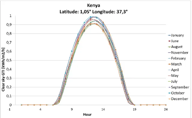
Figure 3.6 - Kenyan location: Clear sky GTI profiles for the first day of each month. . 31

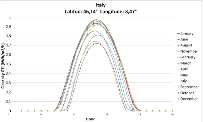
Figure 3.7 - Italian location: Clear sky GTI profiles for the first day of each month... 32

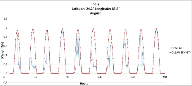
Figure 3.8 - Indian location: real global tilt irradiation profile VS clear sky radiation profile for days of August. ... 36

Figure 3.9 - Kenyan location: real global tilt irradiation profile VS clear sky radiation profile for 10 days of January. ... 36

Figure 3.10 - Indian location: daily clearness index distribution in the month of August. ... 37

Figure 3.11- Kenyan location: daily clearness index distribution in the month of August. ... 38

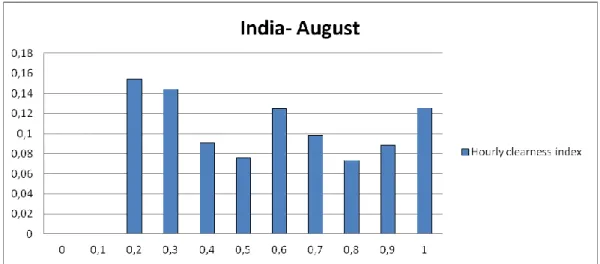
Figure 3.12 - Indian location: hourly clearness index distribution in the month of August. ... 38

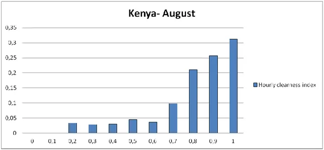
Figure 3.13 - Kenyan location: hourly clearness index distribution in the month of August. ... 39

Figure 3.14 - Indian location: Heat map of the clearness index ... 39

Figure 3.15 - Italian location: Heat map of the clearness index . ... 40

Figure 3.16 - Trends of the monthly power output for different location [MWh/month]. ... 41

Figure 3.17 - Wind Power Global Capacity and Annual Additions, 2005-2015 [12]. .... 43

Figure 3.18 - Weibull probability functions under a constant value of c and different values of k. ... 48

Figure 3.19 - Weibull probability functions under a constant value of k and different values of c. ... 48

iv

Figure 3.20 - Graphical method’s regression. January, India (latitude: 24.2°, longitude: 83.9°). ... 52 Figure 3.21 - Weibull probability density function (pdf) VS wind speed with k=1.3, c=2.03. January, India (latitude: 24.2°, longitude: 83.9°). ... 52 Figure 3.22 - Weibull probability density function (pdf) VS wind speed with k=3.03, c=5.99. August, Kenya (latitude: 1.05°, longitude: 37.3°). ... 53 Figure 3.23 - Probability density functions (pdf) derived from generated data (blue bars) VS Weibull curves built with k and c derived from the graphical method (blue line) VS Weibull curves built with k and c derived from generated data (red line), for different months and locations. ... 58 Figure 3.24 - Dimensionless curves of power coefficient VS wind speed. ... 60 Figure 3.25 - Dimensionless curves of power VS wind speed. ... 61 Figure 3.26 - Mean profile of the dimensionless curves of power coefficient VS wind speed: wind turbines characterized by absent regulation (blue), and variable regulation (green), mean profile between the previous ones (red). ... 61 Figure 3.27 - Mean profile of the dimensionless curves of power VS wind speed: wind turbines characterized by absent regulation (blue), variable regulation (green), mean profile between the previous ones (red). ... 62 Figure 3.28 - General trend of the hub height to diameter with respect to the diameter. . 63 Figure 3.29 - Wind profiles at different hub heights. ... 65 Figure 3.30 - Power output according to wind speed at the hub, for a fictitious day. ... 65 Figure 3.31 - Indian location Lat: 24.2° Long: 83.9°- January 1-2: wind speed at the hub and power output for the first two days of January. Power curve is not linearly proportional with the wind speed curve: the power follows the cube of the velocity. ... 66 Figure 3.32 - Monthly energy production for the three locations. ... 66 Figure 3.33 - Heat map of the hourly power output during the entire year for the Indian location. ... 67 Figure 3.34 - Heat map of the hourly power output during the entire year for the Kenyan location. ... 67 Figure 4.1 - Percentage of irrigated area with respect total cultivated area [71]... 70 Figure 4.2 - Energy required for irrigation in different Indian locations. ... 76 Figure 4.3 - India: Lat: 24.2°-Long: 83.9°: monthly energy required for irrigation and domestic/potable water needs. They represent the programmable portion of the load demand. ... 77 Figure 4.4 - India: Bihar region, January. Irrigation energy requirement [kWh/month], regional averaged data. ... 78 Figure 4.5 - India: Bihar region, January. Effective Precipitations (PE) [mm/month], regional averaged data. ... 79 Figure 4.6 - India: Bihar region, January. Evapotranspiration (ET) [mm/month], regional averaged data. ... 79 Figure 4.7 - India: Bihar region, January. Aquifer depth [m], regional averaged data. ... 80

v

Figure 4.8- India: Bihar region, January. Cultivated area [ha/person], regional averaged data. ... 80 Figure 4.9 - Indian location: Lat: 24.2° Long: 83.9°; productive needs mean daily load profile. ... 83 Figure 4.10 - Basic needs: mean daily load profile. ... 90 Figure 4.11 - Bottom-up and top-down model approaches: bottom-up starts from microscopic data regarding specific load and goes on till aggregated data are computed. ... 92 Figure 4.12 - Examples of working-day load profiles generated with LoadProGen. ... 97

vii

List of Tables

Table 1.1- Access to electricity: world situation [4]... 2

Table 1.2 - Electric outages and duration in developing world macro-regions. ... 2

Table 3.1 - Albedos were calculated for cloud-free conditions using mid-latitude profiles of temperature, humidity, and ozone for summer and winter conditions. ... 29

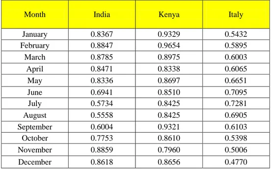
Table 3.2 - Indian, Kenyan and Italian locations: monthly mean daily clearness indices. ... 33

Table 3.3 - STEP matrix. ... 34

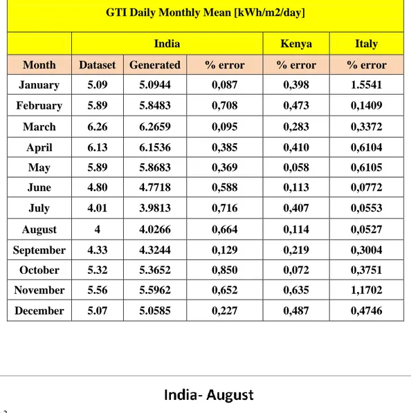
Table 3.4 - Comparison between daily monthly mean latitude tilt radiation data from dataset VS generated: relative errors for the three locations. ... 37

Table 3.5 - Comparison between Weibull monthly parameters derived from graphical method (GM) and Weibull monthly parameters calculated from synthetic generated data series, for the three locations. ... 56

Table 3.6 - Comparison between mean wind speeds from dataset and mean wind speeds calculated from synthetic generated data series, for each month, for the three locations. ... 57

Table 3.7 - List of analyzed turbines. ... 59

Table 3.8 - Friction coefficients for tower height of wind turbines [68]. ... 64

Table 4.1 - Effect of major climatic factors on crop water needs... 72

Table 4.2 - Crops coefficients. ... 73

Table 4.3 - Machinery consumptions. ... 81

Table 4.4 - Coefficients used for the calculation of agricultural residues and wood residues[77]... 85

Table 4.5 - Nominal power of the appliance. ... 87

Table 4.6 - Load factors used for the different appliances. ... 88

Table 4.7 - Basic needs: other hypothesis. ... 89

Table 4.8 - Input data required by the new procedure [89]. ... 91

Table 4.9 - Assumed input data for Load ProGean-Part1. ... 95

ix

Abstract

Access to electricity is still one of the main issues in the world, especially in developing countries. In many cases rural villages are un-electrified and distant from existing national grid networks and they are thinly populated. As a consequence the costs of connection to the grid networks are very high and uneconomical. An established solution is represented by hybrid stand-alone microgrids that are able to provide electricity to the community exploiting local renewable sources.

The most of the times, during the preliminary study of the feasibility and operation of a microgrid in an isolated rural location (simulation phase), precise data regarding load demand are not available. Also local renewable sources as irradiation and wind speed profiles, recorded from the past years, are difficult to be found due to the lack of information and measure equipments.

The purpose of this work is to elaborate a general methodology, focused on rural villages of developing countries but with validity extensible in every location on the earth’s surface, that starting from latitude and longitude coordinates and global datasets, is able to generate hourly annual profiles of load demand and renewable sources power output from the solar PV and wind turbine. These profiles are required as input during the simulation phase.

As regard renewable energy sources, the proposed methods are synthetic data generation models that starting from monthly mean values taken from datasets, they generate 8760 hourly data for the entire year, for the desired location; while regarding load demand, a method for the generation of daily load profiles based on a big amount of assumptions and datasets is suggested; loads are divided into basic needs, agriculture, water needs and productive activities.

All these calculations are implemented with a very flexible and organized Matlab algorithm that requires latitude and longitude as input, and on the basis of many assumptions regarding the type of village, people’s habits, agriculture, productive activities and generators’ characteristics, gives back these three typical annual profiles in addition to other useful information concerning biomass residues.

Keywords: hybrid stand-alone microgrid, synthetic data generation, renewable sources, load demand, input data for microgrid simulation, annual profiles.

xi

Sommario

Ancora oggi, in molti contesti isolati, specialmente nelle zone rurali dei paesi in via di sviluppo, l’accesso all’elettrcità è uno dei problemi principali che influenza lo sviluppo e il miglioramento della vita degli abitanti. La rete elettrica, se presente, è inaffidabile, mentre nella maggior parte dei casi questi villaggi sono lontani dalla rete nazionale e i costi d’investimento per il collegamento sono troppo alti, considerando la relativamente bassa richiesta di energia e la popolazione esigua. Una soluzione nota e consolidata è l’istallazione di minireti ibride isolate, che integrano lo sfruttamento di fonti rinnovabili reperibili in loco, riducendo i costi e la dipendenza da combustibili tradizionali.

Le minireti sono composte da un’integrazione di generatori rinnovabili e non, carichi programmabili e non, e da sistemi di accumulo come batterie, con conseguente grande varietà di configurazioni e applicazioni possibili. In generale le minireti sono una soluzione interessante non solo per villaggi rurali di paesi in via di sviluppo, ma anche in contesti sviluppati quando il collegamento alla rete nazionale è difficile e costoso (per esempio sulle isole, nei deserti, nei villaggi di alta montagna...), oppure possono essere utili in contesti residenziali per integrare le fonti rinnovabili e avere una generazione distrbuiuta propria nel quartiere, oppure ancora in caso di utenze ad alta richiesta di energia come resort per le vacanze.

Ponendo particolare attenzione a villaggi localizzati in zone rurali, i principali obiettivi della minirete sono: la produzione di energia elettrica, garantendo quell’accesso all’energia prima inesistente o poco affidabile, e l’estrazione e pompaggio di acqua potabile e/o ad uso domestico; infatti un altro problema frequente in questi contesti è la mancanza di acqua utilizzabile dalle famiglie, che porta inevitabilmente a problemi sanitari e malattie.

La progettazione di una minirete si articola in tre fasi: simulazione, ottimizzazione e analisi di sensitività. Durante la prima fase, viene simulato un periodo di tempo di funzionamento della minirete in una particolare configurazione (insieme delle taglie dei vari componenti), con un time-step variabile. Tra i dati di input necessari per la simulazione, ci sono i profili annuali su base oraria di potenza prodotta da rinnovabili, quali i pannelli fotovoltaici e la turbina eolica, in quanto dipendono da fattori meterologici (la disponibilità oraria di radiazione solare e vento). Inoltre è necessario un profilo di carico accurato e realistico in relazione ai consumi nella località scelta. Questi dati necessitano di accuratezza nel considerare le dinamiche orarie e giornaliere, al fine di ottenere una soluzione robusta al problema: modellare i carichi e le risorse rinnovabili semplicemente considerando valori medi mensili o medi giornalieri porta invitabilmente ad errori nel dimensionamento dei vari componenti, che saranno sovradimensionati o sottodimensionati, con conseguenti problemi nella risposta della minirete ai vari picchi

xii

massimi e minimi orari di richiesta di energia. In questo lavoro consideremo un periodo di simulazione di un anno e un time-step orario.

Spesso questi dati di input sono sconosciuti per località remote in quanto profili annuali registrati negli anni precedenti non sono disponibili; inoltre le attrezzature per la misura non sono presenti e troppo costose, e il fabbisogno energetico della popolazione non è mai stato indagato o registrato. Durante uno studio preliminare della fattibilità di una minirete in una particolare zona, possono essere utili metodi per la generazione di dati a partire da una serie di ipotesi e dati medi mensili disponibili (mentre i profili annuali sono difficli da reperire, spesso valori medi mensili di varie grandezze sono disponibili praticamente per ogni località sulla Terra). In ogni caso nulla può sostuire un’indagine sul posto. I datasets utilizzati contengono informazioni globali, o in riferimento a una particolare regione/stato di interesse, per ogni valore di latitudine e longitudine.

Lo scopo di questo lavoro è la formulazione di una metodologia, finalizzata alla stima dei profili annuali di input su base oraria, modellizata per contesti rurali in via di sviluppo ma con validità generale in ogni località del mondo. Essa si basa su metodi di generazione sintetica di dati, i quali a partire da valori medi mensili (ad esempio di radiazione solare, ventosità, produttività dei terreni, precipitazioni, ecc...), generano una serie di dati temporali per l’anno intero che rispettino i dati statistici iniziali, e che mostrino una corretta e realistica variabilità giornaliera. Il tutto è stato implementato in Matlab, creando un algoritmo che, una volta decise una serie di assunzioni e ipotesi, leggendo in input solo latitudine e longitudine sia in grado di generare i profili annuali necessari alla futura simulazione.

Per quanto riguarda le fonti rinnovabili, dopo un’ampia analisi dei metodi usati in letteratura al fine di trovare metodologie adeguate ai dataset disponibili, i metodi prescelti vengono proposti e spiegati nella loro formulazione matematica, e i risultati ottenuti vengono analizzati e confrontati con i dati medi mensili inizialmente disponibili. Infine viene eseguita una stima dell’energia oraria prodotta sottolineando pregi e difetti di ogni metodo.

La generazione del carico invece, viene suddivisa in: richiesta di elettricità per l’agricoltura (irrigazione), per l’estrazione di acqua ad uso domestico e trattamenti per renderla potabile, consumi legati ad attività produttive e di lavorazione dei prodotti agricoli, e infine bisogni di base, cioè tutte quelle attività legate alla vita e abitudini degli abitanti (elettrodomestici e carichi vari presenti delle case, nelle scuole, negli ospedali ecc..). Per la generazione del profilo annuale di carico, sono necessarie molte più ipotesi imputabili all’utente rispetto alla parte riguardante le fonti rinnovabili, che si basano più che altro su fattori metereologici. La metodologia utilizzata è particolarmente complessa perchè deve tenere conto dei profili giornalieri di tutti i singoli carichi e delle singole utenze. Infine vi è una sezione riguardante la produzione di resuidi di biomassa dagli

xiii

scarti dell’agricoltura e delle attivià produttive, che possono essere utili per lo sfruttamento in un eventuale generatore a biomasse.

L’algoritmo vuole essere flessibile ad ogni tipo di modifica se dati più accurati sono disponibili o le ipotesi fatte devono essere modificate. In particolare nella costruzione della domanda di carico, tutte le ipotesi fatte devono essere facilmente modificabili e aggiornabili, con la possibilità di una facile introduzione di nuovi carichi, in quanto questi dati sono molto variabili in relazione al tipo di villaggio, alla popolazione, alle attività svolte ecc.

Chapter 1 - Introduction

1 9

1. Introduction

1.1. Access to electricity in isolated contexts

Nowadays access to electricity is still one of the main problems in the world, especially in developing countries. Despite many progresses in terms of electrification in the world are recognizable (in the last decades million of people, before devoid, have electricity now, especially in China and India), it is estimated that up to 1.3 billion of the world’s population have no access to electricity and of these some 97% reside in the world’s developing regions. This situation is most pronounced in sub-Saharan Africa (SSA) where the overall electrification rate is about 33% only, with the rural rate still lower [1], [2].

The positive correlation between access to electricity and development is long established, and although access to electricity in itself is not a remedy for development, modest access to electricity (e.g. lighting) can have substantial benefits on the welfare of the poor. In fact electricity represents one of the main responsible in promoting progress in the society, leading to an improved well-being for people.

Rural areas of developing countries are those which suffer the poorest access to modern energy services; moreover the electric supply system, when available, is often unreliable and it does not reach the majority of the total population. In many cases these rural villages are un-electrified and distant from existing national grid networks and they are thinly populated. As a consequence the costs of connection to the grid networks in terms of fixed costs or per capita costs are very high and uneconomical [3].

An established solution in these situations is represented by off-grid or grid-connected hybrid microgrids that are able to provide electricity to users exploiting local sources.

Microgrids, defined as power systems which include loads, distributed generation, energy storage, and which are managed as a single unit, are becoming a way of integrating renewable energies, lowering costs and providing better grid quality all around the world. Microgrids cover a broad range of scenarios and can be classified as either grid-connected or stand-alone, or according to use: military, industrial, residential etc. Moreover according to their generation sources, they can comprise either renewable generators (typically PV and wind turbines) or fossil fuel-based generators (typically diesel generators or gas micro-turbines). According to all these reasons, microgrids cover a wide range of configurations and goals.

Chapter 1 - Introduction

2

1.2. Electrification: statistical data and global situation

Rate of electrification of rural areas is the lowest as shown in Table 1.1, especially for African countries. The fact that OECD (Organization for Economic Co-operation and Development) countries are almost 100% electrified is remarkable.

Table 1.1- Access to electricity: world situation [4].

Population without electricity [millions] Electrification rate [%] Urban electrification [%] Rural electrification [%] Africa 600 43 65 28 Developing Asia 615 83 95 75 Latin America 24 95 99 81 Middle East 19 91 99 76 Developing countries 1257 76.5 90.6 65.1 Transition

economies & OECD

1 99.9 100.0 99.7

World 1258 81.9 93.7 69.0

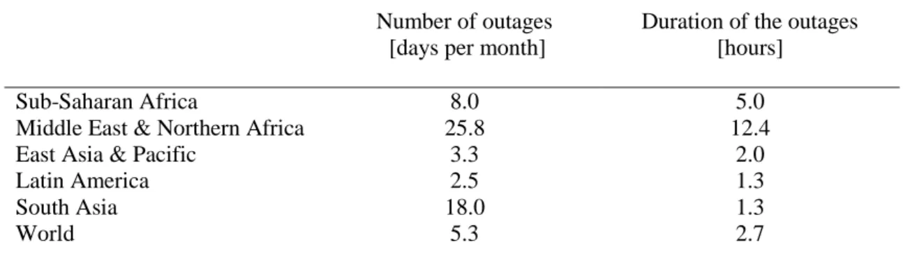
Moreover the electric energy system in the poorest regions, when available, is unreliable. Table 1.2 contains information about electric outages and duration in developing regions [5]. The fact that the electric source is not continuous during the day creates problems to agriculture and productive activities but also schools, hospitals and people’s lives. In rural situations, when there is no access to electricity, population is forced to use traditional biomass, kerosene or small batteries, the most of the time in a very inefficient way

Table 1.2 - Electric outages and duration in developing world macro-regions.

Number of outages [days per month]

Duration of the outages [hours]

Sub-Saharan Africa 8.0 5.0

Middle East & Northern Africa 25.8 12.4

East Asia & Pacific 3.3 2.0

Latin America 2.5 1.3

South Asia 18.0 1.3

Chapter 1 - Introduction

3

A map of the world access to electricity, as a percentage of the entire population with the access, is reported in Figure 1.1. It is clear that locations that mostly require a solution in terms of electricity supply are India and Sub-Saharan African countries, as said at the beginning (light blue region).

Figure 1.1 - World access to electricity (% of population with the access) [6].

Indian situation

Only in India, 450 million of people are without electricity access. Despite the striking increase in power generation capabilities, India has been unable to keep up with its domestic demand for electricity for many years. India’s transmission and distribution infrastructure is inadequate to meet future demand. Some disparities occurred in the last years: a preference for industries and urban electrification, neglecting rural supply: in light of these disparities, new policies were introduced to reform the electricity sector. Figure 1.2 shows the village electrification rate in 16 big states from 1970 to 2000. Some states as Kerala, Tamil Nadu, Haryana and Punjab already had a high level of electrified villages in the early 1970s and completed all village electrification before 1980. However there are states as Orissa, Uttar Pradesh, West Bengal, Bihar and Assam, whose electrification process stagnates in the 1990s before being complete. These are the states that are more interesting from point of view of microgrid installation, since

Chapter 1 - Introduction

4

there is still an electricity access request. Today 85 % of Indian villages are electrified, but fewer than 60 % of households actually consume electricity [7].

Figure 1.2 - Electrification rate in 16 big Indian states from 1970to 2000.

African situation

African situation is the worst. Although the total African population is 16 % of the entire world population, it represents half of the world population without access to electricity (Figure 1.3). Most of the African continent is still in the dark after nightfall: this fact creates big issues as regard growth of the activities, medicines and vaccines refrigeration, livelihoods. Today 25 countries in sub-Saharan Africa are facing a crisis due to continuous blackouts. Despite the availability of renewable sources and fossil fuels, they are not well distributed creating big disparities among countries. The main issues are [8]:

- Low access and insufficient capacity: 24 % of the population of sub-Saharan Africa has access to electricity versus 40 % in other low income countries. Excluding South Africa, the entire installed generation capacity of sub-Saharan Africa is only 28 GW, equivalent to that of Argentina.

- Poor reliability: power outages very frequent, as a result enterprises lose sales revenues during these periods of time.

- High costs: power tariffs in the rest of developing world fall in the range of US$0.04 to US$0.08 per kilowatt-hour, while in these regions the average tariff is

Chapter 1 - Introduction

5

US$0.13 per kilowatt-hour. In countries dependent on diesel-based systems, tariffs are still higher.

Figure 1.3 - Distribution of population without access to electricity in African regions [9].

1.3. Developing countries VS developed contexts electrification

In developing countries, the most of the times, microgrids find application in rural settings to ensure electricity access, as widely explained before. But a microgrid, in general, can be useful not only in rural settlements of developing countries but also in all these cases where the access to the grid is difficult or in general the long-term costs can be reduced: for example an island not grid-connected to the coast or high altitude isolated mountain villages; in addition they find application also for residential buildings or district solutions.

Islands and remote communities

Microgrids installed in developed countries meet different requirements with respect developing ones. Stand-alone renewable microgrids can be installed in different isolated locations as islands, high mountain villages or desert areas far from urban areas, in order to face different problems:

Chapter 1 - Introduction

6 - high costs of connection to the coast;

- high costs derived from the use of oil-based microgrids; - environmental considerations: reduced global emissions; - abundant local resources.

[10] presents 10 cases of study about renewable microgrids installed on islands around the world. It explores examples of communities transitioning from one resource (oil) to a diverse set of resources including wind, solar, biodiesel, hydro and energy storage. Some microgrids are small and they serve fewer than 100 people, others over 10000 people with a peak demand range from 60 kW to 27 MW. Figure 1.4 shows a map of these locations.

Figure 1.4 - The 10 reviewed microgrids [10].

Residential/urban solutions

In some cases the adoption of microgrids is not due to the lack of electricity access, which would be guaranteed by the government, but rather for other reasons. For example resorts can exploit a grid-connected microgrid, for reliability reasons, to produce the big amount of energy requested on their own, with lower costs with respect to buy it from the grid and with the possibility of absorbing electricity in case of high demand. Moreover in case of locations characterized by intermittent supply due to overloads or network unbalance, they guarantee a continuous service to their customers. Residential microgrids can be installed to integrate renewable sources (as PV panels and small wind turbines) with the district, balancing demand and supply, organizing and optimizing electricity networks locally. They have been increased popularity thanks to new energetic policies promoting distributed generation and ‘Nearly Zero-Energy Buildings’,

Chapter 1 - Introduction

7

buildings that have a very high energy performance and significant production from renewable energies. [11] reports an example of an existing residential microgrid.

1.4. Rural electrification: off-grid VS grid-connected systems

About 70 % of the world’s poor people live in rural areas. For improving their situation it is essential to improve their access to goods, services and information. Due to low initial costs, accessibility and simple operation, diesel generators have been the technology of choice for initial electrification. However the increasing fuel cost, together with additional increasing costs of transportation in such remote areas, makes the diesel generators too expensive for providing reliable electricity supply in the long run. Microgrids are a good solution from point of view of sustainable energy supply, transition away from fossil fuel dependence and mitigation of rural poverty.

Focusing on rural applications in developing countries, the energy demand is generally low. Concerning poor villages, families own only few appliances, a lot of public services are not present, specific equipments of hospitals or schools are very simple: so the cost of connection to the national grid represents a very big investment, in most of the cases uneconomical. Sometimes also political and social problems arise: for example in Ghana, there is ample evidence that un-electrified communities in low income countries prefer to be connected via the grid. Many communities perceive off-grid technologies as inferior due to their availability and limited supply, or the access to off-grid technologies is seen as a transition to grid technology. In reality these community preferences for grid-electrification are linked to politicians’ promises of grid access during political campaigns, and related investments [3]. Anyway stand-alone hybrid microgrids, in many cases, remain the only feasible solution.

1.5. Renewable sources integration

In even the most remote areas, renewable energy is increasing access to basic energy services, including lighting and communications, cooking, heating and cooling, water pumping, etc., generating economic growth. PV household systems, wind turbines, micro-hydro powered or hybrid mini-grids, biomass-based systems or solar pumps, and other renewable technologies are being employed in homes, schools, hospitals, agriculture, and small industries in rural and off-grid areas of the developing world.

The number of rural households served by renewable energy is difficult to estimate as the sector becomes driven increasingly by individual project promoters or private

Chapter 1 - Introduction

8

companies, but it runs into the hundreds of millions. Off-grid renewable solutions are increasingly acknowledged to be the cheapest and most sustainable options for rural areas in much of the developing world. This will have an impact on market development in the long term. They allow for power production with negligible operation costs and no environmental impact. They are extremely attractive in rural contexts where the sustainability of the project is fundamental. Off-grid systems are typically based on renewable sources thus reducing dependency on fossil fuels, they are modular and hence can be adapted to different rural energy needs, and they are located near to the consumers [12]. Figure 1.5 is the global heat map of renewable microgrids progress.

The challenge of stand-alone hybrid microgrid is the integration of renewable generators with other traditional generators and accumulation systems. This fact is particularly interesting since renewable sources are usually available in loco (sun, wind and in some cases biomass), and the exploitation of these energies in place of fuel-based generators leads to money savings in terms of costs of purchase and transportation.

Moreover developing countries as sub-Saharan African (SSA) countries are lucky from point of view of the high solar potential and in some locations of wind availability.

Chapter 2 - Design of a rural microgrid

1 9

2. Design of a rural microgrid

2.1. Main targets of a microgrid

In this work we focus on a rural stand-alone microgrid for developing countries. The microgrid is made of different components: generators, loads, an accumulation system and an inverter. Figure 2.1 shows an example of layout: in general PV panels and the battery/accumulation system work in DC current, while wind turbine and the other dispatchable generators work in AC current, so an inverter is required.

Figure 2.1 - Microgrid’s layout.

The main targets to be achieved are:

- Electric energy supply: thanks to the microgrid the access to electricity is ensured to many users as households, hospitals, schools, farms and so on. Electricity can improve not only the lifestyle of people but also many activities connected to agriculture and all the related production activities that will no longer be carried out manually.

- Domestic/Potable water supply: electricity can be also exploited to withdraw water from the soil and make it potable, representing a great way to improve the quality of life. Most of the times potable water is not available in developing rural areas, creating sanitation problems. According to a joint report by UNICEF and

Chapter 2 - Design of a rural microgrid

10

the United Nations, of the 783 million people still without safe drinking water, 40% lives in sub-Saharan Africa [14]. Figure 2.2 illustrates where the roughly 11 percent of the world population without the benefit of safe drinking water resides.

-

Figure 2.2 - World population without access to safe drinking water (millions).

2.2. Design of a microgrid: phases

The design of a microgrid is made of three phases: simulation, optimization and sensitivity analysis.

- During simulation, a size for each component is chosen and a useful period of time of operation for each generator and accumulation system is simulated. Their behavior depends on the chosen control strategy or dispatching strategy, meaning the way each component works with the others. A monitoring of the moments a component is switched on/off, of the fuel consumption and of the battery charge/discharge is achieved. A typical period of time for simulation is one year, while the time step can vary; in this work we assume a time step of one hour and a total period of time of one year, but these parameters are flexible: in some cases user is interested only in a specific period of time. Anyway, testing the operation of the microgrid on the long span is important to evaluate the operation costs. Equally important is the study of the response of the various generators to different maximum and minimum peaks of demand: for this reason a reliable

Chapter 2 - Design of a rural microgrid

11

profile of load demand is important for a proper sizing of the generators and batteries. Simulation represents the inner level of analysis.

- Optimization means finding the optimal combination of components and components’ sizes according to one particular parameter (for example LCOE-Levelized Cost Of Electricity, or others…), repeating the simulation phase and comparing the different results. So, in this phase some economical comparisons are made and also the best dispatching strategy can be selected. Optimization represents the external level of analysis.

- During sensitivity analysis some initial assumptions are changed and the optimization process is repeated. In this way the influence of each parameter can be analyzed. Changing some initial assumptions also the result of the optimization phase can change: the importance of precision about the initial assumptions is tested. This phase is a sort of further outer level.

It is clear that during each time step, the feasibility of the microgrid needs to be studied: loads must be satisfied and constraints regarding the generators or the battery must be respected.

2.3. Design methods

Design methods, based on efficient operation strategies, have been widely studied in literature. Either well-known available software or possible self-implemented algorithms, used for the design and the management of a microgrid are usually based on one of these kinds of methods:

- Average methods: they use simple, algebraic equations to make the necessary evaluations. Only average values are used: daily load consumption and average monthly energy production from renewable sources. Running time is surely very low, due to simple calculations, with the possibility to make a lot of performance evaluations about different configurations, but they do not represent precisely the real situation: considering only mean values, information about peaks and daily variability are lost, leading to possible over-sizing or under-over-sizing of the different components.

RETScreen is a Clean Energy Project Analysis Software system based on

average method, jointly developed by the Government, Industry and Academia of Natural Resources Canada in 1996. The purpose is the renewable energy and cogeneration project feasibility analysis as well as ongoing energy performance analysis. It is able to evaluate the energy production and savings, costs, emission reductions, financial viability and risk for both isolated and grid-connected projects (examples of applications in literature [15], [16]).

Chapter 2 - Design of a rural microgrid

12

RETScreen is a scenario tool, performing comparison between the conventional case and an alternate “clean energy” one, thanks to economical indicators as IRR and NPV. The output is a simple approach, investments costs are optimized very quickly because it uses monthly time steps. Some advantages of this model are that it allows for a multiple number of generators, its ease of use and user-friendly interface. One limitation which is known is its inability to model any storage systems [17].

- Simulation methods: these kinds of methods try to reproduce the real behavior of the microgrid, using a lower time step (e.g. hour, 15 minutes…). Comparing different configurations according to a desired parameter (LCOE, RES penetration...), the optimal one is found. Using hourly time-step, a better representation of reality with respect to average methods is achieved, since daily dynamics are considered, but running time clearly increases.

HOMER is maybe the most famous, reliable and well-established software

used for the design of a microgrid: it is a micro-power optimization model that can be used to evaluate, in a simplified way, both off-grid and grid-connected power systems for a variety of applications. These optimization and sensitivity analysis algorithms simplify the decision of the best system configuration: which components it makes sense to include and what size. To use HOMER, some inputs must be provided, which describe technology options, component costs, and resource availability. HOMER uses these inputs to simulate different systems configurations, or combinations of components and generate a list of feasible configurations sorted by net present cost. Also a wide variety of graphs and tables are reported. It simulates the operation of a system by making energy balance calculations for each of the 8760 hours in a year. For each hour, HOMER compares the electric and thermal demand in the hour to the energy that the system can supply in that hour, and calculates the flows in the hour to and from each component of the system. In the presence of a battery it also decides when charge or discharge the battery. It performs these calculations for each system configuration desired determining whether a configuration is feasible and whether it can meet the electric requirements specified; moreover it can estimate the costs of installing and operating the system [18].

The drawback is the non-predictive strategy (Load Following or Cycle Charging) used: the result is strongly influenced by the initial data. A possible improvement is achieved with the optimization of these initial parameters.

- Capacity planning methods: methods belonging to this group, reach the simultaneous optimization of optimal operation and design of a microgrid.

Chapter 2 - Design of a rural microgrid

13

They are usually adopted for large grids but can be applied also to smaller grids, stand-alone or grid-connected.

DER-CAM (distributed Energy Resources Customer Adoption Model): the

most popular commercial software based on this method. It is an economic model developed by LBNL (Lawrence Berkeley National Laboratory), capable of finding the best possible combinations of technologies, the optimal capacity and operation profile that meet the microgrid’s electrical and eventual thermal loads. The optimization is done a priori, for given utility tariffs, fuel cost and other equipment data. DER-CAM is a General Algebraic Modeling System (GAMS) based on Mixed Integer Linear Programming (MILP) model. It is mainly used for three different types of applications: to make choices of equipment adoptions at specific sites or hypothetical sites; it provides reliable basis for the operations of installed on-site system; it can be used to assess the market potential of technologies by anticipating which kinds of costumers might find various technologies attractive. EAM is a similar tool that, in opposition to DER-CAM, involves a Mixed Integer Non-Linear Programming (MINLP) model, because a non-linear consumption of fuel is considered. [17] describes also other models developed and presented in literature.

2.4. Input data: renewable sources and load demand

Irrespective of the type of existing software or self-implemented algorithm used, some input data must be provided. Assumptions regarding the components (investment cost, efficiency, etc.) are set at the beginning, as much realistic as possible according to the application, and they usually remain equal during the simulation phase. Moreover they are easy to be managed and changed if necessary. But there are other input data requested to proper simulate the power flows at each time step and for this reason they need to be as much accurate and realistic as possible during the entire period of time:

- Load demand: the annual load profile is required for an accurate simulation of the microgrid’s behavior. In a rural context different daily loads must be taken into consideration and from their aggregation a daily load profile for each day is considered, characterized by different peaks during the day depending on the season, week-day/ festive-day, people’s habits and so on. It is important to introduce variability day by day and hour by hour to better simulate the real functioning.

- PV power production: an annual radiation profile and consequently the PV power output annual profile is very important for the proper sizing of the photovoltaic panels. Irradiation is different every hour of the day and every day of the year, for

Chapter 2 - Design of a rural microgrid

14

every location on the earth. For this reason simply considering a mean monthly value or mean daily value repeated over time steps is not correct: it can lead to overestimation or underestimation of the power flows during each time step, and consequently to overestimation or underestimation of the components’ sizes.

- Wind power production: a value of wind speed for each time step is important for the same reasons explained for solar irradiation. In particular the wind turbine power output is not linearly dependent on the wind source, so small wind speed fluctuations are preferable to be taken into consideration instead of using average values, equal at each time step.

Taking into account hourly variability is very important to achieve a robust and reliable solution at the end of the process. Using mean monthly values or mean daily values, leads to missing information about real maximum or minimum peaks and the future inability of the components to follow the actual load consumption’s dynamics. As accurate as possible input data profiles are desired over the entire simulation period.

2.5. Objective: annual profiles reconstruction from latitude and

longitude coordinates

Focusing on rural applications in developing regions, the availability of input profiles of load and renewable energy sources, is one of the main issues during the starting phase of the microgrid design. As regard the load curve, the better solution would be the collection of information directly on site: from documentations if available, talking with people, doing interviews about their habits and consumptions, looking at the activities for their livelihoods. While, as regard renewable resources, the better solution would be the availability of annual meteorological profiles derived from local recorded measurements from past years. The most of the times these data are not available and hard to come by isolated rural regions due to the lack of measuring equipments or the difficult leakage of information from remote and poor areas: only monthly mean information are findable. So a method for the reconstruction of such annual profiles from averaged data is needed, valid for every location on the earth’s surface. It can’t substitute in any way a local survey but it is useful for a preliminary study.

The objective of this work is the reconstruction of input annual profiles of renewable generators’ power output and load demand, on hourly basis, starting from latitude and longitude coordinates. To do that, synthetic data generation methods are applied, which reconstruct time data series from averaged values.

Chapter 2 - Design of a rural microgrid

15

A Matlab algorithm is implemented, that requires as input latitude and longitude, and gives back as output the three desired data series (Figure 2.3) and other useful information. To do that the algorithm requires some initial basic assumptions to be completed characterized by high flexibility, in the sense that input hypothesis can be easily changed, according to the kind of application. Some databases, containing information about world meteorological data, land’s productivity etc. as a function of latitude and longitude, are introduced by the algorithm and exploited to make a lot of calculations. Also these datasets can be easily substituted in any moment with more reliable or with a higher resolution ones. The advantage of this method is that datasets contain monthly mean information for every value of latitude and longitude on the earth’s surface, or related to the specific considered country; so, also for those remote locations where measured data do not exist, hourly annual profile can be rebuilt.

Figure 2.3 - Flowchart of the algorithm.

In this work we pay particular attention on rural applications for developing countries when dealing with the loads definition, but the proposed method has a general validity in any location, as already stressed, and so the algorithm can be exploited for all those remote areas with difficult input data investigation.

Chapter 2 - Design of a rural microgrid

Chapter 3 - Renewable sources

1 9

3. Renewable sources

3.1. Renewable generators

In this chapter we want to pay particular attention on renewable sources and their availability curve during a year. The presence of renewable generators allows the reduction of the dependency on fossil fuels, since they exploit a primary energy that is available in loco. This is always true for solar and wind energy, while in case of biomass the issue is a bit more complicated.

Photovoltaic panel/panels and the wind turbine/turbines (for sake of simplicity only one component is considered since we are dealing with a general methodology to evaluate the power output and not the specific size or technology/machine used), are non dispatchable generators. They are characterized by quite high investment cost but low operating costs and environmental impact. Non dispatchable means that power is produced only when the primary energy source is available (sun or wind), and they are not regulated by the power management system. They are intermittent and aleatory, which means that they are not continuously available due to factors outside direct control as weather parameters. The main reason that solar power is non-dispatchable is the fact that Sun does not shine for all hours of the day in a given location, in addition to the problem of cloud coverage. Also wind power is highly intermittent because of the variability of wind speed, and the turbine characteristics that require wind within a certain range to generate electricity. The world availability of solar and wind energy are shown in Figure 3.1 and Figure 3.2.

Figure 3.1 - World solar potential on a horizontal plane [19].

Chapter 3 - Renewable sources

18

Figure 3.2 - Mean wind speed: world distribution [20] .

Notice that third world areas such as India or sub-Saharan African countries, that are the most probable locations for a microgrid installation, are characterized by good values of irradiation, especially African countries. As regard wind, in India mean speed values are not so high; the situation is about the same in Africa except for the Sahara desert and some other countries, with very low wind speed in the central region (blue region). So the solar PV will be surely well exploited, while wind turbine needs to be examined more in detail.

Biomass generator is dispatchable, since it is linked to the presence of a fuel and it can produce electricity when requested by the control system. All the dispatchable generators are fundamental to compensate for the intermittency of renewable sources, ensuring load fulfillment. In general it is reasonable to assume that the presence of the biomass generator depends on the availability of biomass sources (residues from forests, residues from agriculture, etc…) in the surrounding region. Biomass exploitation is usually economically advantageous when the resources are present in the nearness because: the costs of transportation are low (in some cases it is made by hand), transportation could be difficult especially in case of remote sites, the exploitation is worthwhile from a social point of view since residues from agriculture and production activities, are not wasted. So biomass generator is worthwhile for two reasons: it is a renewable, green generator, almost neutral from point of view of emissions, and thanks to its dispatchability it can theoretically substitute the diesel generator in balancing non-dispatchable RES generators. In some poorest situations, biomass residues, as wood or agriculture crops, are used as domestic fuel to cook and heat, in a very inefficient way; so an analysis of the residues in the surrounding is important: this part will be treated in chapter 4, when dealing with agriculture energy demand and soil productivity.

Chapter 3 - Renewable sources

19

3.2. Solar radiation

Solar energy is the portion of the sun’s energy available at the earth’s surface for useful applications. This energy is free, clean, and abundant in most places throughout the year. Solar power is a suitable source because of the high solar radiation available especially in many developing countries and the low maintenance requirements. The interest for solar power has also increased in other parts of the world because of the need of more environmental friendly power generation to both the future power demand and the survival of our planet.

Solar PV experienced a record growth in 2015, with the annual market for new capacity up to 25% over 2014. More than 50 GW was added, equivalent to 185 million solar panels, bringing total global capacity to about 227 GW. The annual market was nearly 20 times the size of cumulative world capacity just a decade earlier (See Figure 3.3). Until recently, demand was concentrated in rich countries; now, emerging markets on all continents have begun to contribute significantly to global growth, with solar PV taking off where electricity is needed most: in the developing countries [12].

Figure 3.3 - Solar PV Global Capacity and Annual Additions, 2005 [12].

Solar radiation that reaches the earth is called extraterrestrial solar irradiation (above the atmosphere), while the attenuated solar radiation within the atmosphere is called global solar radiation. Global solar radiation incident on a horizontal surface has two

Chapter 3 - Renewable sources

20

components, namely, direct (beam) and diffuse solar radiation; the latter one is the fraction of extraterrestrial radiation that is scattered in the atmosphere. Both components are usually measured by pyranometers; direct radiation can be also measured by a pyrheliometer, while diffuse radiation by placing a band over a pyranometer.

To get the most from solar panels, they need to be pointed in the direction that captures the most sun when the solar radiation arrives perpendicularly upon the surface. There are a number of variables in figuring out the best direction: latitude, day of the year, tilt angle, azimuth angle, time of the day, angle of incident radiation. Moreover the total radiation incident on a tilted surface is also a function of the ground reflected radiation. Prediction of the global irradiance incident on such tilted surfaces is a key feature for the evaluation of the solar resource and the performance of all these systems.

In this work the panel is assumed fixed, since the microgrid is usually made of simple, small size components; so the tracking system can result too expensive for this kind of applications. To obtain maximum annual energy availability from a fixed tilted panel, a surface slope equal to latitude is the optimal solution and the surface should face the equator. It means the solar collector in southern hemisphere should face the north and vice versa [21].

The clearness index is an important parameter in the description of solar radiation: it is defined as the ratio of the solar radiation recorded on the earth’s surface to the extraterrestrial solar radiation, and it can be defined on hourly basis, daily basis or monthly average daily basis; the last one is useful in this work according to the input data available.

The monthly average daily clearness index is the ratio of monthly average daily radiation on a surface to the monthly average daily extraterrestrial radiation:

(3.1)

The daily clearness index is the radiation in a day to the extraterrestrial radiation for that day:

_(3.2)

An hourly clearness index can be also defined for a specific hour:

Chapter 3 - Renewable sources

21

3.2.1. ‘Typical meteorological year’ (TMY) profile

‘Typical meteorological year’ (TMY) is one of the most common synthetic weather data sequences used as input for a microgrid. Electrical generation by solar energy needs detailed site-specific data for designing or modeling the performance of the solar panel. In fact solar energy varies over a broad range of space and time scales because of the complex dynamic evolution of clouds.

TMY of weather data usually consists of 12 months of hourly data. Each month is selected from long-term weather data as being the best representative of the particular month or it is generated from several years of weather data which would yield the same statistics (such as the average solar radiation and clearness index).

State of art would be the availability of a database with TMY profiles for any latitude and longitude locations on the earth. Examples of suitable datasets are:

- TMY3, it is a directory containing the data files for the typical meteorological year data derived from 1961-1990 and 1991-2005 National Solar Radiation Data Base archives of US.

(http://rredc.nrel.gov/solar/old_data/nsrdb/1991-2005/tmy3/).

- Satel-light, the European Database of Daylight and Solar Radiation, provides real measured data in hourly values, over 5 years (1996-2000) for any pixel of 5x7 km2 in Europe.

(http://www.satellight.com/core.htm).

- NREL lists where to find many weather resource data, on yearly basis for many locations, in the form of SAM weather files that are text files that contain one year’s worth of data describing the solar resource, wind speed, temperature and others.

(https://sam.nrel.gov/weather)

3.2.2. Synthetic data generation

The issue is that these archives listed in the previous section, contain information only about specific sites, where weather stations or measurement equipments are present. Historical solar radiation data, taken at high sampling frequencies, are unavailable for many locations where solar radiation measurements are not possible because of not being able to afford the measuring equipments and techniques involved.

So, there are situations that force to the use of mathematically or synthetically generated time series that employ stochastic methods for constructing a synthetic time

Chapter 3 - Renewable sources

22

series of irradiance data. These kinds of methods try to fill the gaps between generally available data resources and the parameters requested by solar applications.

Starting from datasets containing information about monthly mean solar radiation as a function of latitude and longitude, our purpose is to find a method able to generate 8760 hourly radiation data for every location on the earth, to be used in the microgrid operating simulation. If simple monthly mean values of radiation derived from dataset are used, simulation does not take into account all night hours or all that hours/days of wide clouds coverage characterized by very low PV energy production, but even the peak hours where the radiation is much higher with respect to the mean: a wrong PV sizing can result. The model has to introduce an hourly and daily variability, over all the yearly profile, maintaining the statistical information about the monthly means.

3.2.3. Literature review

There is a wide scenario of proposed models for synthetic irradiance data generation in literature. Various models can be used, depending on the time resolution (e.g., hourly or monthly mean) and on the type of available input data (e.g., meteorological information about global irradiance on the horizontal, on a tilted surface…).

A lot of models have been analyzed in this study, a brief description of the most important is reported below. Hourly solar radiation data distributions can be estimated or fit into stochastic models such as Auto-Regressive (AR) [22], Auto-regressive Moving-Average (ARMA) [23], Markov matrix approach [24], [25], or other systems such as Neural Networks [26], [27], [28], that are the most validated models. Many of them are commonly used for both solar irradiation and wind speed synthetic data generation.

Autoregressive models (AR)

The use of autoregressive models is reported in literature very commonly. The first-order autoregressive [AR (1)] model takes into account only the effect of the previous value in the series of the observed sequence of data . This sequence is

used to fit a model of form:

(3.4)

where is the hourly mean wind speed, the autoregressive coefficient that is a model parameter, and a normally distributed independent random variable. Notice that Eq. (3.4) is written for the mth order. The simulation procedure for the process is very simple: it requires only a random number from a normal distribution to be generated.

Chapter 3 - Renewable sources

23

Autoregressive model can increase in order and the dependence structure in the observations is better preserved [29].

To use this method, a sequence of observed data is needed for every

latitude/longitude coordinates, for this reason is not suitable for our purposes. Auto-regressive Moving-Average models (ARMA)

ARMA is a type of time-series analysis that can be used in situations that deal with a large amount of observed data from the past. The ARMA system is developed using Eq.(3.5) and consists of two parts, the auto-regressive (AR) part and the moving average (MA) part.

(3.5)

is the forecasted solar irradiance at time t. In the AR part, p is the order of the AR process, and is the AR coefficient. In MA part, q is the order of the MA error term, is the MA coefficient and ) is the white noise that produces random uncorrelated variables with zero mean and constant variance.

Typically, this method requires large amount of historical data to find the orders p, q and the coefficients and . In addition, due to the geographical differences, each location requires its own unique coefficients. The mathematical methods of finding the orders and coefficients of the ARMA architecture are introduced in [30].

Markov models

Many authors propose Markov Transition Matrix (MTM) methods to model the clearness index, the global irradiance or other parameters of interest. Markov models provide a simple yet powerful way of modeling the dependence between adjacent observations in a given time series. A process is said to exhibit the Markov property if, given its present state, the future is conditionally independent of the past and Markov models are mathematical representations of such stochastic processes.

A Markov process ( , t=0,1,2,…) with a set of m allowed states (1,2,…,m) is said to be in state j at time t if . In practice, given the dataset, the observations are divided into states (if the observations range between 0 and 1, state 1 can be defined between 0 and 0.01, state 2 between 0.01 and 0.02...).

In a first order Markov process, given that the process is in state i at time t-1, the probability that it will be in state j at time t is given by a fixed probability written mathematically as:

Chapter 3 - Renewable sources

24

(3.6)

, known as the transition probability from state i to j, is independent from the states

of the process at times t-2, t-3, etc. In a nth order Markov model, the probability that the process will be in a particular state at time t depends not only on its state at time t-1, but also on the states at times t-2, t-3,…,t-n. In a second order Markov process, the probability that the process will be in state k at time t is given by:

(3.7)

For a process with m allowed states, the first order transition matrix would typically be represented as:

(3.8)

While the second order transition matrix is:

(3.9)

Similarly, an nth order Markov model will have a transition matrix.

From a given set of observations, the transition probability from state i to j can be easily estimated by counting the number of times the states sequence ij is observed and dividing by the total number of times state i is observed. For the second order process calculation is the same but considering the sequence ijk. In this way Markov transition matrices and cumulative probability transition matrices can be constructed.

Considering a first order matrix, with elements all between 0 and 1, to generate the sequences of states, the initial state, say i, is selected randomly. Then random values