Dynamical models for pedestrian dynamics using data from pedestrian flow sensors

Alma Mater Studiorum · Universit`

a di Bologna

Scuola di Scienze

Dipartimento di Fisica e Astronomia Corso di Laurea in Fisica

Dynamical models for pedestrian dynamics

using data from pedestrian flow sensors

Relatore:

Prof. Armando Bazzani

Correlatore:

Prof. Alessandro Fabbri

Presentata da:

Tommaso Marzi

Abstract

The purpose of this thesis is to give a contribution in a wider project regarding the development of new tools for the governance of tourist flows in Venice. Because of the virus COVID-19, this topic has increased in interest, since it can be used both to look for possible solutions to make public places safer and to study the spread of the virus itself.

Once the testing of the sensors that provide the data on mobility is carried out, a macroscopic approach to the pedestrian dynamics based on the Fundamental Diagram is proposed: scenarios with different geometries as streets, crossroads or bridges are compared, focusing in particular on representative parameters of the model.

In the last part, a microscopic approach to pedestrian mobility is presented: a simulation model is calibrated on the basis of the available data, in order to define whether it can actually reproduce the behaviour of a crowd.

Abstract

Questa tesi rappresenta un contributo a un progetto pi`u ampio riguardante lo sviluppo di nuovi strumenti per la gestione dei flussi turistici a Venezia. A causa del virus COVID-19, questo argomento ha acquisito un ruolo ancor pi`u centrale nella societ`a, dato che permette sia di ricercare soluzioni per rendere i luoghi pubblici pi`u sicuri, sia di studiare la propagazione del virus stesso.

Inizialmente verr`a effettuato il collaudo dei sensori che forniscono i dati sulla mobilit`a. Successivamente, da tali dati verr`a proposto un approccio macroscopico alla dinamica pedonale basato sul Fundamental Diagram, analizzando in particolare scenari con diverse geometrie come strade, incroci o ponti in relazione ad alcuni parametri rappresentativi del modello.

Nell’ultima parte, verr`a effettuata la taratura di un modello simulativo sulla base dei dati disponibili, al fine di verificare se un approccio microscopico pu`o riprodurre in maniera accurata il comportamento di una folla.

Acknowledgments

I would like to thank VENIS (Venezia Informatica e Sistemi S.p.A.) for the collaboration in providing the data and L. F. Davoli and P. Birello, with whom I have worked closely during the realization of this thesis.

Contents

Abstract i

Introduction 2

1 Pedestrian models 4

1.1 Microscopic models . . . 4

1.2 Macroscopic models and Fundamental Diagrams . . . 5

2 Testing of the sensors 9 2.1 The data available . . . 9

2.2 Preliminary data analysis . . . 11

2.3 Reconstruction of counts from flows . . . 15

2.4 Anomalies detected in the data acquisition . . . 19

3 Fundamental Diagrams 20 3.1 Operational definition of the Fundamental Diagram . . . 20

3.2 Fundamental Diagrams in different scenarios . . . 21

3.2.1 Madoneta (FP035) . . . 22 3.2.2 San Felice (FP025) . . . 24 3.2.3 San Rocco (FP036) . . . 26 3.2.4 Maddalena (FP006) . . . 28 3.2.5 Canonica (FP014) . . . 30 3.2.6 Callelovo (FP019) . . . 32

3.2.7 Comparison of the results . . . 34

4 Calibration of a simulation model 37 4.1 The simulation approach . . . 37

4.2 Calibration in Madoneta . . . 38

Conclusions 41

Introduction

Walking is an essential aspect of our everyday life. As a matter of fact, even if only par-tially, it is always included in every human movement, regardless of the distance traveled. This reality leads to the necessity to examine in depth the so called pedestrian mobility to improve several aspects of cites, both socially and economically: pedestrian mobility makes a massive contribute to the liveability of a city, also making it more hospitable for tourists. Moreover, if connected to a well-planned public transportation network, it produces a positive impact on environment and climate, by reducing emissions of private vehicles and improving the quality of air.

Studies on pedestrian mobility are covered by complex systems, since the collective be-haviour of the crowd emerges from the interactions between the single individuals. For this reason, the purpose of physicists is to build models that take into consideration both the dynamics of the system, which can be associated to the dynamics of a granular flow, and the cognitive processes of pedestrians. In particular, an important aspect on which research is focused consists of the emergent behaviours, that are the consequences of the self-organizational predisposition of the crowd, e.g. the tendency of two opposite flows of people in a corridor to organize themselves in two defined lanes [1].

The association of the crowd to a granular flow allows not only to study the pedestrian mobility, but also to find a solution to panic situations in closed spaces: pedestrian mod-els are often used to find strategies to avoid dangerous circumstances typical of public spaces, e.g. situations related to maximum capacity of scenarios as the bottleneck effect [2], that is a clogging effect that occurs when the whole crowd tries to get out from a place by passing through a single door. In this type of situation, the psychological state of individuals is a key aspect in the discussion of the evolution of the system. Indeed, the level of panic of the crowd can lead to paradoxical effects, as the freezing by heating [3], that is the formation of a blocked situation from a state of disorder comparable to the formation of a crystal, or the faster is slower effect [3][4], that is a phenomenon of slowdown due to the crowd attempting to evacuate as quickly as possible.

Obtaining information from the analysis of the behaviour of pedestrians is not trivial. As a matter of fact, while in vehicle traffic rules are strict and well defined, in pedestrian traffic, except from isolated cases like traffic lights, they are more flexible and several variables are involved. In particular, the trajectory of individuals does not have to follow

a definite path as for the vehicles, but it changes over time depending on the dynamics of the whole crowd and, furthermore, the study of pedestrian mobility must consider the variability of individuals: velocity is heavily dependent on characteristics like age, health or fitness. These examples show only a small part of the complexity in studying this field.

This thesis represents a contribution to a new project that focuses on the tuning of a predictive model of pedestrian mobility in Venice, a unique city of its kind which has been for years a tourist attraction centre and it is nowadays the headquarters of world-famous events. Since the city is built on water, pedestrian traffic is further complicated due to the fact that it is characterized by frequent critical points: just think about the fact that the old town includes more than 100 islands connected with more than 400 bridges and tight streets or crossroads can be frequently encountered.

In the first chapter general literature on several types of pedestrian models is presented, focusing in particular on basic notions and parameters which will be useful in the fol-lowing chapters. Problems and considerations related to the influence of the scenario are proposed.

In the second chapter the available data are presented and the testing of the sensors that provide them is carried out, highlighting any problems.

The third chapter analyzes the characteristics of pedestrian mobility for various loca-tions, focusing in particular on representative parameters of the model.

In the fourth chapter a comparison is made between the data and a simulation approach to verify if the latter can reproduce and accurately predict the behavior of a crowd.

Chapter 1

Pedestrian models

Despite pedestrian mobility is a field that began to develop only in the second half of the 20th _{Century, several approaches to study it have been defined, each of them with}

their strengths and weakness. Since it is a recent topic there is not yet one model that is preferred to other models because they are deeply dependent on the application to which they refer, but they can be divided into microscopic and macroscopic models according to the approach adopted.

1.1

Microscopic models

Microscopic models describe crowd dynamics in terms of the dynamics of single individ-uals: the result of interactions among pedestrians provides the collective behaviour of the crowd. In particular, the dynamics of a single individual are based on the avoid-ance of collision with other pedestrians and obstacles. Microscopic approach includes different types of models that vary from the first attempt with discrete models to the most advanced analytical models. In particular, the basic discrete model is the Cellular Automata defined by P. Gipps and B. Marksjo in 1985 [5], in which space is represented with cells that assume different values depending on whether there is an obstacle, a pedestrian or the very cells are empty. As well as space, in this matrix-based system time is also discrete, allowing to perform a simulation that is not expensive in terms of computation and can be approximated as a continuum for small time increments. By adding rules to make the evolution of discrete systems more precise, Agent Based Models [6] are created: they give a more detailed description related to the discussion of pedestrians as single agents with precise behaviour rules that share a common space, but paying the price of a higher computational expenditure.

Microscopic models include also equation-based models that, unlike discrete models, give an analytical description of pedestrian mobility. In particular, the Social Force Models [3] describe the dynamics of each pedestrian as a superposition of two types of forces:

at-tractive forces, provoked by the desire to walk with a certain speed or reach a particular place, and repulsive forces, provoked by the presence of other pedestrians or obstacles. This model can be improved by introducing geometrical parameters that reproduce the real dynamics of walking, as an angular dependence in repulsive forces to exclude in-teractions with pedestrians that are not seen. Moreover, as reported by Bin Yu et al [7], the social force model can be expressed in terms of fields: this formulation allows us not to be forced to consider two entities as in the case of the dissertation with forces, since individuals move following a dynamics that is the interaction between individuals themselves (which can be considered as a charge) and a pre-existing field. On the other hand, the real perception of interaction with other pedestrians and obstacles needs a more complex discussion.

1.2

Macroscopic models and Fundamental Diagrams

The central concept of macroscopic models is to describe the dynamics of individuals through an average behaviour of the crowd, using physical quantities like mean density ρ and mean flow Φ. These quantities are both functions of time and space and they are related to each other in the equation of continuity, which can be obtained by considering the crowd as a continuum and treating it as a compressible fluid:

∂ρ(x, t)

∂t + ∇Φ(x, t) = 0 (1.1) Moreover, the mean flow can be written as: Φ = ρ(x, t) · v(ρ), where v(ρ) represents the average velocity of the system. This last relation between the mean quantities is the main topic of interest of macroscopic models and it defines the so called Fundamental Diagram (FD), which represents the behaviour of pedestrians as a function of density. As consequence of Equation 1.1, FD can be expressed in an equivalent way as v(ρ), Φ(ρ) or v(Φ). As reported by Vanumu L.D. et al [8], FD has a strong dependence on several factors, in particular on the flow type, the scenario considered and the characteristics of the crowd, like country of origin or age. Despite this variability, crowds made up of different types of individuals and in different environments share common shapes in FD. In particular, in Figure 1.1 Fundamental Diagrams obtained from several studies are reported, including scenarios with different geometries such as sidewalks and walkaway (Tanariboon et al [9]) or analysis on streets with different widths (Older [10]). Moreover, in the figure analytical results are also reported as the one of Weidmann [11], which aims to reproduce several FDs in different circumstances with a functional dependent on characteristic parameters.

Figure 1.1: Fundamental diagrams of pedestrian flow characteristics resulting from em-pirical data obtained in different configurations of flow and facilities (Daamen et al [12]). Taking v(ρ) into consideration, it can be noticed that velocity is inversely propor-tional to density as expected and, for low values of density, different flows follow the same trend even if with different values of speed, while for high values of density, velocity de-pends on the crowd considered. Moreover, FD highlights two important quantities that are heavily dependent on the flow characteristics and the environment: a critical value of density ρcrit(density at capacity) where the system resides in a stationary regime with

low values of velocity (traffic congestion) and an optimal value of velocity vf ree which

corresponds to the speed when there are no other pedestrians in the area (free speed ). Considering FD in the equivalent forms, the observations remain the same and the cor-responding values of ρcrit in terms of speed (speed at capacity) and flow (capacity flow )

can be defined. These values have been collected and compared for several crowds and facilities by T. Kretz [13] and they are reported in Table 1.1: these researches include both studies obtained from empirical data, like those mentioned above, and experiments conducted in laboratory. Regarding these latter, in Table 1.1 is reported the one of Jin et al [14], conducted in a circular corridor for different types of flow, and those of

Hanking and Wright [15], where they compared data obtained from a tube station (HW Commuters) to those obtained from an experiment conducted in the same setup of Jin et al (HW Boys).

Indeed, literature on pedestrian mobility obtained from empirical data is often combined with experiments in laboratory, since different samples of empirical data do not always reproduce the same behaviour because of the variability of the crowd and the environ-ment. On the other hand, we must take into consideration that the values obtained from experiments are generally higher than those obtained from real data, since distractions present during a walk which can affect the velocity or the trajectory are not considered: for example, an individual can slow down or even stop if she/he sees a tourist attraction or a showcase of her/his interest.

Capacity Density at Speed at Free Experiment flow capacity capacity speed

[1/m · s] [1/m2] [m/s] [m/s] Weidmann 1.22 1.75 0.7 1.34

Fruin 1.25 1.97 0.64 1.34 SFPE 1.32 1.9 0.69 1.20 PM Adults Summer normal 1.69 7.5 0.23 0.91 Helbing et al 1.83 3.99 0.46 1.22 Lohner et al 2.91 8.0 0.36 1.45 HW Commuters 1.99 4.37 0.46 1.62 HW Boys 2.28 5.38 0.42 1.49 MT 2.32 3.65 0.64 1.47 Older 1.31 2.51 0.52 Jin et al 1.63 2.13 0.77 2.00 Table 1.1: FD’s parameters obtained from several studies and collected by T. Kretz [13].

The flow type and the scenario mentioned by Vanumu L.D. et al are strictly related, because in most cases the former is determined by the latter: for example, if the scenario is a corridor, the flow will be consequently uni-directional or bi-directional depending on whether the corridor is accessible from both directions; if the scenario is a crossroad, the flow will not have a definite path due to the several possibilities of route and, without

restrictions, it will be multi-directional.

In this regard, it is useful to mention the experiments conducted by S. Motsch et al [1]: trajectories of people moving in two opposite directions in a circular corridor are traced and from these the Fundamental diagram is obtained. Moreover, a self-organizational behaviour of the crowd has emerged from data, that is the formation of two lanes. This effect has a strong dependence on initial conditions: in case of flows with the same quan-tity of pedestrians (50% - 50%) the pattern of the two lanes is well defined, while the removal of the initial balance of the two directions causes a progressive decrease of this effect. This phenomenon is a consequence of the collective intelligence of the crowd and it depends on the habits of individuals (e.g. right-hand or left-hand drive rule of each country).

In the series of experiments conducted by S. Cao et al [16] regarding crossroads, FD for different types of flow is obtained from two different methods, one based on the Voronoi Diagram and the other one on a counting method. The former is a geometric subdivision of space into cells, where each of them contains only the points that are closer to the individual associated with that very cell, in comparison to other individuals. A local density and a local velocity are associated with each cell and by integrating these quan-tities on all the surface FD is obtained. The latter is based on the counts obtained by four barriers positioned at the four entrances of the crossroad and it allows to highlight the possibility of count several times a single individual during traffic congestion. This problem occurs because of the multiple trajectories doable by the individual to reach her/his goal.

A phenomenon that often occurs is the stop and go waves [17], which are an intermittent flow due to situations of congestion: this behaviour shows up both for small and large time intervals and two phases coexist at the same time. In particular, a constant accel-eration and slowdown of individuals is recorded according to their position and therefore velocities vary with wide fluctuations over the time. Regarding these latter, a study conducted by E. Andreotti et al [18] on vehicle traffic highlighted that fluctuations be-gin to occur before the density reaches its critical value and therefore the actual ρcrit is

lower than the theoretical one. Moreover, a behaviour of self-organization of the crowd decreases these fluctuations, bringing the system to the stable state.

Critical situations are heavily dependent on the psychological state of individuals, which can cause unexpected effects such as freezing by heating [3] and faster is slower [3][4]. The former is a transition of the system to a stuck situation that occurs for high densi-ties: when the general state of panic is high, the crowd does not behave like a disordered system, but paradoxically it enters in a state similar to a crystal where individuals oc-cupy fixed positions. The latter occurs when people tries to get out through a single exit in panic situations: individuals aim to get out as soon as possible, causing an increase of the friction among other pedestrians which leads to a decrease of the velocity. The result is therefore a increase of the exit time, hence the name of this effect.

Chapter 2

Testing of the sensors

2.1

The data available

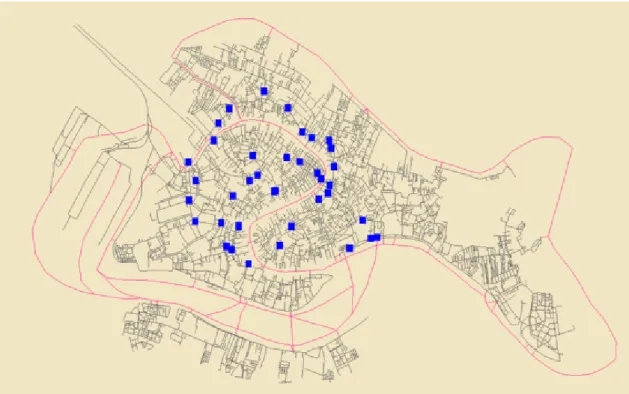
The project aims to treat Venice’s pedestrian traffic as broadly as possible. In order to achieve this goal, 33 detection sensors belonging to the brand Xovis have been placed (Figure 2.1), that trace pedestrians’ trajectories and provide their position every 0.25 s. Measurements are assumed as highly precise and there is no associated error.

Subsequently these positions are analyzed, providing different types of data: a simple counting data with a sampling of one minute and a data referring to flows with a sampling of five seconds. The former is increased whenever an individual crosses a barrier and it is an exact value (for each barrier there are two counters depending on the direction in which it is crossed), while the latter consists of a directional count in the eight directions of the compass rose with the associated mean speed (provided in dm/s). In particular, the flow data are calculated by attributing the movement of each individual to the direction traveled the most among the eight octants in 5 seconds, where each octant is identified as the circular sector between the direction with which the name is associated and the nearest direction by turning clockwise (e.g. the north octant is the sector between north and north-east). Once attributed, the counter in that direction is increased and the corresponding velocity is averaged with those of the other individuals in that direction. Moreover, there is a third type of data which corresponds to the total number of presences in the area obtained from the flows. Obviously, fixed individuals do not contribute to velocity field, but they are still counted in presences. In Figure 2.2 an example of a scenario with the associated barriers is reported.

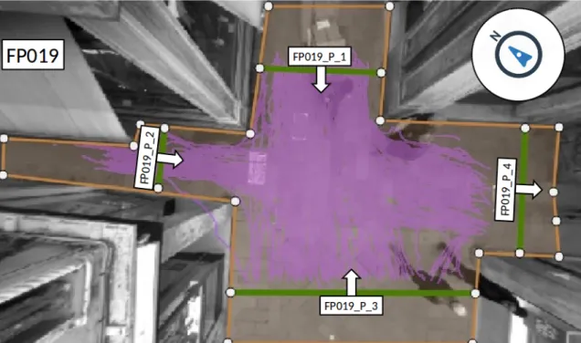
Figure 2.2: View of sensor FP019, that records the crossroad between Calle del Lovo and Calle dei Fabbri. The area enclosed by the orange polygonal chain is the area where the sensor traces pedestrian and the compass defines the north and consequently the octants. The green segments indicate the barriers and the associated arrow the IN/OUT direction. The violet lines indicate the trajectories of individuals.

The sensors work in specific lighting conditions and consequently during dark hours the data are not reliable; moreover, since they track heads of pedestrians moving in the area, they are sensible on weather conditions because the use of umbrellas can obstruct the proper operation of the camera. Sensors recognize an individual from her/his height, in particular with a minimum height of 1m.

2.2

Preliminary data analysis

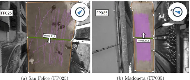
Before starting with the construction of the model, the truthfulness of data provided by the sensors has been verified. In particular, sensors San Felice (FP025 - Figure 2.3a) and Calle de la Madoneta (FP035 - Figure 2.3b) were used to perform the test. This choice was dictated by the fact that both of these scenarios are relatively simple to study, since they are corridors and consequently the flow will be mostly bi-directional. Moreover, the counting problems presented in the previous chapter are not valid.

(a) San Felice (FP025) (b) Madoneta (FP035)

Figure 2.3: View of the sensors in San Felice (FP025) and Madoneta (FP035) with their north and barrier orientations.

The geometrical parameters of these sensors are reported in Table 2.1; these estimates may not be accurate, because as seen in Figure 2.3 the trajectories of individuals are not tracked in the whole area, probably due to boundary effects and moreover the barrier length is not given. Consequently, a scale factor may be required.

Sensor Area [dm2_{] Barrier length [dm]}

San Felice (FP025) 10300 70 Madoneta (FP035) 2030 25

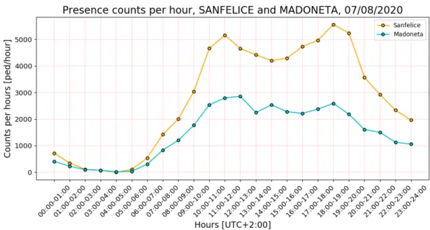
Table 2.1: Geometrical parameters of San Felice (FP025) and Madoneta (FP035). The variability of the number of people recorded during the day reflects the behaviour of an individual with a regular routine, with certain restrictions related to the case considered. In Figure 2.4 the presences of the the two sensors during a weekday are reported: a significant number of people begins to register in the morning, when people usually start working. This number rises until it reaches a peak during lunchtime and, after a slight decrease in the early afternoon, it peaks again in the evening. After the setting of the sun, which is around 20:30, the counts may no longer be reliable. The same observations hold for non-working day with the appropriate changes.

Figure 2.4: Presences per hour recorded by the sensors in San Felice (FP025) and Madoneta (FP035) on Friday 07/08/2020.

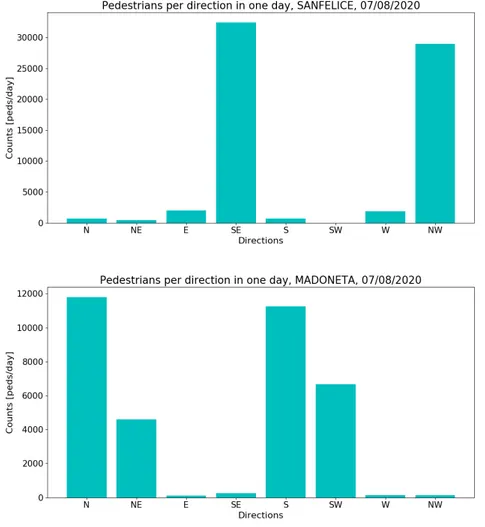
In Figure 2.5 the counts per direction recorded by the sensors on Friday 07/08/2020 are reported: it is clear that in San Felice (FP025) there are two preferential directions, that are NW and SE, while in the other directions there are non-zero counts, except for SW where there might be a problem in the data recording. However, we can assume that its contribution in the total flow is marginal since SW is not a preferential direction.

Even though this street is wide, the trajectories of individuals usually follow a linear path, except for deviation due, for example, to the desire to stop in front of shop windows: this fact justifies the large difference in counts between the preferential direction and the others. Referring to Figure 2.3, it can be noticed that, unlike San Felice, in Madoneta the compass rose is not centered in a defined direction, but it is an intermediate way between N and NE for the IN direction and S and SW for the OUT direction. The counts per direction in the histogram of Madoneta in Figure 2.5 validate this consideration. Moreover, although it is a narrow street, it ends in another street orthogonal to it, forming a crossroad: this region is not registered directly by the sensor FP035, but it influences the counts in reference to the directions according to the desire of individuals to choose a certain direction at the intersection.

Figure 2.5: Pedestrian counts per direction registered in San Felice (FP025) and Madoneta (FP035) on Friday 07/08/2020.

To estimate the value of vf ree in both scenarios the regime with the lowest density is

considered, that is the regime when only an individual is recorded in the eight directions in five seconds. In particular, for both the sensors this method is applied on the period 03/08/2020 - 17/08/2020 and the average values of velocity with the number of entries of the samples are reported in Table 2.2:

Sensor vf ree [dm/s] Entries

San Felice (FP025) 11.44 ± 0.02 21044 Madoneta (FP035) 11.87 ± 0.02 30778

Table 2.2: vf reewith the number of entries of the samples for both sensors. The associated

errors are the standard deviations of the mean of the samples.

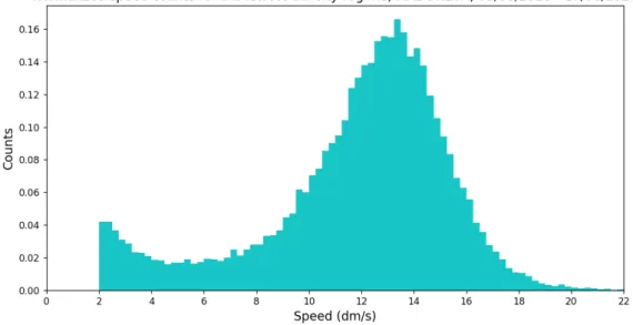
These values are comparable with those of literature reported in Table 1.1, which are between 9dm/s and 20dm/s depending on the flow considered. In Figure 2.6 the normalized distributions of the two samples in low density regime are reported: it is evident that the lowest bound of velocity is set to 2 dm/s and individuals that move with lower speed are considered as stationary. The distribution of vf ree can be assumed

as a normal distribution with a mode that is higher than the mean value reported in Table 2.2, but still comparable with the values reported in literature. Single counts with extremely high speeds that may be linked to runners or cyclists are not shown in the graph.

Figure 2.6: Normalized distribution of velocity in the regime of lowest density for San Felice (FP025) and Madoneta (FP035) recorded on the period 03/08/20 - 17/08/2020.

2.3

Reconstruction of counts from flows

Once it has been verified that the flow data are reliable, we can proceed to reconstruct the counts provided by the barriers of both sensors from the flow data using an analytical approach. Let ˆνb with b = IN, OU T be the versors of the two directions of a barrier and

let ˆek with k = 1, ..., 8 be the versors of the eight octants. The number of people passing

through the barrier in the sense b per unit of time will be defined as: Φb(t) = l A 8 X k=1 θ(ˆek· ˆνb)vk(t)nk(t) (2.1)

where l and A are respectively the length and the area reported in Table 2.1, vk(t)

and nk(t) are respectively the mean speed and the counts at the time t in the direction

k given by the flow data and θ(x) is a function defined as: θ(x) =

(

x if x ≥ 0 0 if x < 0

It is immediate to see that ˆek· ˆνb, which is the argument of θ(x), is equal to cos(α),

where α represents the angle between the two versors. Consequently, as expected, in the reconstruction of the counts of a barrier b only the octants in the same sense of b provide non-zero contribute. These octants correspond to the directions with α ∈ [−π₂,π₂].

Moreover, since in both the sensors taken into account the scenario is a corridor, ˆνOU T =

−ˆνIN holds.

Since flow data are provided with a sampling ∆t = 5 s, the total counts in a given time interval T = N ∆t will be:

Cb(T ) ' Z t+T t Φb(t) dt = N X n=1 Φb(n∆t)∆t (2.2)

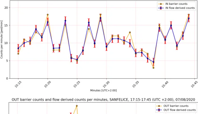
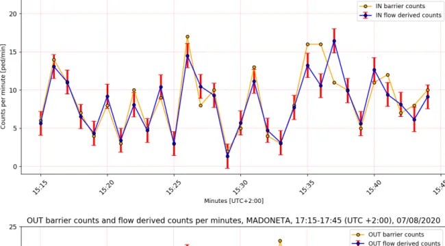
In Figure 2.7 and Figure 2.8 the comparisons minute by minute between counts from barriers and counts derived from Equation 2.2 are reported: in FP025 the angle between the IN and SE directions is 22.5◦ and it is equal to the angle between OUT and NW, in FP035 the angle between IN and NE directions is 7.5◦ and it is equal to the angle between OUT and SW. The error associated to the counts deriving from flow data is calculated as the average deviation between the reconstructed value and the expected value, that is the value of the barrier. Despite the high precision required and the roughness of the calculation, the derived values follow in a fairly good way the barrier values and taking into account the fact that both the geometric parameters and the angles may not be precise, a relatively good flow data accuracy can be assumed.

Figure 2.7: Comparison between barrier counts and counts derived from flow data in San Felice (FP025) between 17:15 and 17:45 (UTC+2:00) on 07/08/2020. The associated error is 1.08 ped/min.

Figure 2.8: Comparison between barrier counts and counts derived from flow data in Madoneta (FP035) between 17:15 and 17:45 (UTC+2:00) on 07/08/2020. The associated error is 1.58 ped/min.

2.4

Anomalies detected in the data acquisition

Since sensors are operative all day long and they continuously provide large quantities of data, they need to be often restarted: this procedure usually occurs during the night, when, as stated before, the sensors do not allow a correct acquisition due to insufficient light. However, connection errors or other types of malfunction can lead to a forced restart.

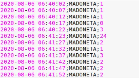
The analysis of the sensors that will be exposed in the next chapter has revealed another type of problem in two scenarios, that are Callelovo (FP019) and Madoneta (FP035). In particular, taking into consideration a period of two weeks, a quantity of data equal to a total period of 8 hours was not recorded. If compared to the other four sensors in analysis, that in the same period were turned off for 24 minutes, the data not recorded by Callelovo and Madoneta are a significant amount. Moreover, by analyzing in depth these periods - which are usually less than 2 minutes long - it turned out that, before the operation resumes correctly, an anomalous data is provided: in Figure 2.9 is reported an example of this type of data in the database of the presences. The sensor provides the data with a sample of 5 seconds with an offset of 2 seconds from the zero. In particular, we can notice that at the time 06:40:22 the sensor stops providing data and it resumes the next minute, precisely at the time 06:41:23, that does not correspond to the normal frequency of output. Moreover, the value provided is 24 pedestrians in the area, which, considering the time slot in which it is calculated, it is most likely an incorrect value resulting from the accumulation of data in the previous minute.

Therefore, in the following chapter, during the discussion on Madoneta and Callelovo, high values of density with low occurrences will not be taken into consideration since they are not reliable.

Figure 2.9: An example of anomalous presence data provided in the time instant imme-diately following the resumption of the correct operation of the sensor in Madoneta.

Chapter 3

Fundamental Diagrams

3.1

Operational definition of the Fundamental

Dia-gram

The easiest way to define the Fundamental Diagram from flow data is to express it as v(ρ), where the density is equal to the number of pedestrians NP ed(t) at the time t in

the recorded area:

ρ = NP ed(t) A =

P8

k=1nk(t)

A (3.1)

Consider a certain density ρ and let ti with i = 1, .., Mρ be the time instants in the

interval [t0, tf] such that:

8 X k=1 nk(ti) ≡ 8 X k=1 nik= ρA (3.2)

holds, or rather Mρ is the number of occurrences of ρ in the time interval. Note that,

according to the data available, the time increment in [t0, tf] will be ∆t = 5 s. The mean

modulus of velocity associated to ρ will be defined as: v(ρ) = 1 Mρ Mρ X i=1 ( P8 k=1viknik P8 k=1nik ) = 1 MρρA Mρ X i=1 8 X k=1 viknik (3.3)

where vik refers to the modulus of velocity in the direction k at the time instant ti.

As stated above, fluctuations of velocity are signals of critical situations and they can be related to traffic congestion, slowdowns or turbulence phenomena. To estimate these fluctuations one can define the sample standard deviation associated to the velocity v(ρ) as:

σv(ρ) = s 1 Mρ PMρ i=1 P8 k=1nik· (v(ρ) − vik)2 ρA (3.4)

Indeed, this definition of the sample standard deviation in terms of a weighted mean of the squared deviation of the velocity in the eight directions is an approximation due to the impossibility to calculate the deviation between the average velocity and the velocity referred to the single pedestrian, since the sensors provide the speeds already averaged on the counts in the eight directions.

The error associated to v(ρ) is the standard deviation associated to the mean and it is defined as: ¯ σv(ρ)= σv(ρ) pρAMρ (3.5)

3.2

Fundamental Diagrams in different scenarios

In order to analyze different geometries, six distinct sensors have been taken into con-sideration: the already known San Felice (FP025) and Madoneta (FP035), one street named San Rocco (FP036) of intermediate size between the two just mentioned, one bridge named Maddalena (FP006), one crossroad with three entrances between Calle de la Canonica and Calle de l’Angelo (FP014) and the crossroad with four entrances between Calle del Lovo and Calle dei Fabbri (FP019).

In the following subsections the FDs related to each of the six sensors are determined by using Equation 3.3 in a time interval of two weeks, that is the period 03/08/2020 -17/08/2020. At first, the FDs will be presented for each scenario and basic parameters as vf ree, vmin and the slope obtained from the linear regression are discussed. Regarding

the latter, it will be performed without considering the first points corresponding to low density regimes, where the dynamics is similar to the one of free motion. Moreover, if the occurrences of a certain number of pedestrians are not sufficient to establish the validity of the data, the correspondent velocity is not considered in the regression.

Secondly, the FDs will be compared with each other in relation to the scenario consid-ered. The errors associated to velocities are calculated through Equation 3.5. Moreover, through Equation 3.4 fluctuations of velocity will be discussed.

3.2.1

Madoneta (FP035)

The Fundamental Diagram obtained in Madoneta (Figure 3.1) with its associated linear regression is reported in Figure 3.2. The area recorded by the sensor is 20.3 m2.

In this scenario, vf ree = (1.187±0.002) m/s and as expected it linearly decreases with the

increase of the number of pedestrians to a minimum value of vmin = (0.762 ± 0.011) m/s,

which corresponds to a density of 0.99 m−2, that is 20 pedestrians. Since for higher numbers of individuals the values of velocity are no longer reliable because of the problem mentioned in the previous chapter, a critical regime of congestion cannot be established. From the linear regression on the data a slope S = −0.349 m3/s was obtained. The hypothesis of a linear relation in the stable regime between the velocity and the density is confirmed by a coefficient of determination R2 _{= 0.972.}

The standard deviation - reported in Figure 3.3 - assumes as well a decreasing trend with the rise of density and it is heavily dependent on both density and Mρ: a higher number

of occurrences leads to an increase of the variability in the values of speed and, moreover, when there is less people in the area, the heterogeneity of the individual behavior can significantly increase the value of deviation. Indeed, this heterogeneity is not recorded for high densities, since in these cases pedestrians are forced to slowdown.

Figure 3.1: View of the sensor in Madoneta (FP035) with its north and barrier orienta-tions.

Figure 3.2: Fundamental Diagram of Madoneta (FP035) obtained with Equation 3.3 in the period 03/08/20 - 17/08/20. The straight line obtained through the linear regression has equation: v(ρ) = −ρ · 0.349 m3_{/s + 1.084 m/s. The reported errors are obtained with}

Equation 3.5.

Figure 3.3: Fluctuations of velocity in Madoneta (FP035) obtained with Equation 3.4 in the period 03/08/2020 - 17/08/2020.

3.2.2

San Felice (FP025)

In Figure 3.5 the FD obtained from the sensor in San Felice (Figure 3.4) is reported. The optimal value of speed is vf ree = (1.144 ± 0.002) m/s. In this scenario a definite

critical value cannot be proposed: as a matter of fact, there is no significant deviation from the linear decrease of the velocity. Nonetheless, this happens only when the speeds corresponding to densities higher than 0.33 m−2, that is 34 pedestrians, are not taken into consideration, in which the number of occurrences is not sufficient to establish the validity of the data. This observation can be justified referring to the geometry of the street: the area has a value of 103 m2 and the total counts recorded in 5 seconds in the period considered are not enough to reach a possible critical value. As a matter of fact, the value of maximum density recorded - that is the value when there are 38 pedestrians in the area - is 0.37 m−2 and it is extremely low if compared with those of literature (Table 1.1). The minimum value reached is vmin = (0.842 ± 0.011) m/s and it

is obtained when 34 pedestrians are in the area.

The sample corresponding to the density of 0.35 m−2, that occurs for 36 individuals, contains only a time instant in which the flow is distributed in five directions (NW, W, S, SE and E): in particular, the greatest part of pedestrians move in NW with a velocity vN W = 1.089 m/s - which is as expected less than vf ree - and they generate in

the opposite flow a slowdown, but the former make up most of the flow and therefore the average speed is still high.

The slope obtained from the linear regression is S = −0.464 m3/s and the coefficient of determination R2 _{= 0.887. The latter is lower than the one of Madoneta due to the}

point correspondent to a density of 0.31 m−2 (32 pedestrians), where, despite it is not negligible, it deviates from the trend significantly.

Since critical situations are not recorded, the fluctuations of velocity do not assume significant values: the linearity of the FD is confirmed by the trend of the standard deviation as a function of density reported in Figure 3.6. In particular, the standard deviation decreases without assuming values that differ significantly from the trend: since San Felice is a wide street, no critical values are reached and, in case pedestrians have to change the trajectory, they can choose between several paths without having to stop. The only data on which considerations can be made is the one discussed above where 36 pedestrians are recorded and where the sample standard deviation assumes a value of σ36 = 0.229 m/s. However, this value cannot be connected to signals of a critical

Figure 3.4: View of the sensor in San Felice (FP025) with its north and barrier orienta-tions.

Figure 3.5: Fundamental Diagram of San Felice (FP025) obtained with Equation 3.3 in the period 03/08/20 - 17/08/20. The straight line obtained through the linear regression has equation: v(ρ) = −ρ · 0.464 m3/s + 1.001 m/s. The reported errors are obtained with Equation 3.5.

Figure 3.6: Fluctuations of velocity in San Felice (FP025) obtained with Equation 3.4 in the period 03/08/2020 - 17/08/2020.

3.2.3

San Rocco (FP036)

In Figure 3.8 the FD obtained from the sensor in San Rocco is reported. A value of opti-mal speed vf ree = (1.215±0.002) m/s deriving from the above mentioned FD is obtained.

The area of the scenario (Figure 3.7) is 36.5 m2 and the same considerations proposed for San Felice are valid: a value of critical density cannot be established since the data allow to analyze a maximum value of 0.60 m−2. Moreover, the velocity decreases with the number of pedestrians without assuming values that deviate significantly from this trend. This fact is also confirmed by the fluctuations of velocity reported in Figure 3.9, which also decrease with the density without giving signals of congested regime.

The minimum value of velocity reached, which corresponds to a density of 0.55 m−2, that is 20 pedestrians, is vmin = (0.801 ± 0.014) m/s and it is not comparable with those of

literature (Table 1.1).

Despite for densities higher than 0.45 m−2 the values begin to deviate from the decreas-ing trend, the coefficient of determination assume a value of R2 _{= 0.908. The slope}

Figure 3.7: View of the sensor in San Rocco (FP036) with its north and barrier orienta-tions.

Figure 3.8: Fundamental Diagram of San Rocco (FP036) obtained with Equation 3.3 in the period 03/08/20 - 17/08/20. The straight line obtained through the linear regression has equation: v(ρ) = −ρ · 0.510 m3/s + 1.128 m/s. The reported errors are obtained with Equation 3.5.

Figure 3.9: Fluctuations of velocity in San Rocco (FP036) obtained with Equation 3.4 in the period 03/08/2020 - 17/08/2020.

3.2.4

Maddalena (FP006)

In Figure 3.11 the FD obtained from the sensor in Maddalena (Figure 3.10) is reported. It records an area of 40.6 m2_{. Since this scenario is a bridge, the height difference}

caused by the stairs affects the value of velocity and indeed the optimal value of speed is vf ree = (0.990 ± 0.002) m/s, which is lower than the values obtained previously.

The minimum value of velocity obtained - which corresponds to 22 pedestrians - is vmin = (0.67 ± 0.02) m/s and it is comparable to the critical speed reported in Table 1.1.

This number of pedestrians occurs in three different time instants and in each of them a wide variability is recorded, both in the directions covered and in the associated velocities: this heterogeneity is related to geometry of the bridge, in particular to its height difference and its curvature. Indeed, an individual which walks through it in a sufficiently slow way to be recorded in more than one time instant, she/he may will be associated in different directions during her/his crossing. The value of vmin might suggest that for this number

of pedestrians the system is in a transitional regime and is evolving towards the critical regime, but on the other hand the correspondent density is 0.54 m−2, which is lower than the critical values reported in literature. Moreover, the fluctuations of velocity - reported in Figure 3.12 - confirm this hypothesis by showing no signals of critical situations: there is no value that deviates significantly from the decreasing trend.

The analysis of the linear regression provided a slope S = −0.266 m3/s, with a coefficient of determination of R2 _{= 0.856, probably due to the points which deviate from the linear}

Figure 3.10: View of the sensor in Maddalena (FP006) with its north and barrier orien-tations.

Figure 3.11: Fundamental Diagram of Maddalena (FP006) obtained with Equation 3.3 in the period 03/08/20 - 17/08/20. The straight line obtained through the linear regression has equation: v(ρ) = −ρ · 0.266 m3_{/s + 0.891 m/s. The reported errors are obtained with}

Figure 3.12: Fluctuations of velocity in Maddalena (FP006) obtained with Equation 3.4 in the period 03/08/2020 - 17/08/2020.

3.2.5

Canonica (FP014)

The optimal value of speed obtained from the Fundamental Diagram reported in Fig-ure 3.14 is vf ree = (1.090 ± 0.003) m/s. The area of the entire scenario (Figure 3.13)

is 39 m2 _{and consequently the intersection between the two streets where the}

interac-tion of pedestrians has a greater influence will certainly be less. Without considering the values corresponding to densities higher than 0.65 m−2, since they have only one occurrence and therefore such data may not be reliable, the minimum value of velocity is vmin = (0.687 ± 0.013) m/s and it corresponds to 24 pedestrians, that is a density of

0.62 m−2. As in the previous cases, the data do not allow to define a value of ρcrit: it

would be necessary to observe the behaviour of the system when there are more individ-uals in the area in order to detect a critical situation.

The vmin is comparable to the speeds of congestion reported in Table 1.1 and, as in

the case of Canonica, we can assume that the system is a transitional regime. How-ever, vmin occurs for a density lower than the critical values reported in literature and,

moreover, the trend of the fluctuations of velocity - reported in Figure 3.15 - is coherent with this consideration. Supposing that the value of the area is not overestimated, this observations can be justified by assuming that the geometry of the crossroad influences the behaviour of the crowd: the intersection between the two streets and the possibility of an individual to choose between several trajectories increase the interaction between pedestrians and therefore velocities are more sensible to density.

The coefficient of determination R2 = 0.956 confirms the linear trend and the associated slope has a value S = −0.491 m3_/s.

Figure 3.13: View of the sensor in Canonica (FP014) with its north and barrier orienta-tions.

Figure 3.14: Fundamental Diagram of Canonica (FP014) obtained with Equation 3.3 in the period 03/08/20 - 17/08/20. The straight line obtained through the linear regression has equation: v(ρ) = −ρ · 0.491 m3/s + 0.977 m/s. The reported errors are obtained with Equation 3.5.

Figure 3.15: Fluctuations of velocity in Canonica (FP014) obtained with Equation 3.4 in the period 03/08/2020 - 17/08/2020.

3.2.6

Callelovo (FP019)

In Figure 3.17 is reported the FD resulted from the sensor in Callelovo (Figure 3.16), from which a value of optimal speed vf ree = (1.074 ± 0.003) m/s is obtained. The area

of this scenario is 69.2 m2 and the same observation regarding the geometry of Canonica can be proposed.

The trend of the velocity for the stable regime decreases with a slope S = −0.594 m3_/s

and it is confirmed by the coefficient of determination R2 = 0.969.

If we consider densities with more than one occurrence, the minimum value of velocity is vmin = (0.773 ± 0.006) m/s and it corresponds to 24 pedestrians, that is a density of

0.35 m−2. This value is higher than those of congested speed reported in literature and therefore we can assumed that the system is distant from the critical regime.

The fluctuation of velocity reported in Figure 3.18 are coherent with this hypothesis, since they not assume wide deviation from the trend.

Figure 3.16: View of the sensor in Callelovo (FP019) with its north and barrier orienta-tions.

Figure 3.17: Fundamental Diagram of Callelovo (FP019) obtained with Equation 3.3 in the period 03/08/20 - 17/08/20. The straight line obtained through the linear regression has equation: v(ρ) = −ρ · 0.594 m3_{/s + 0.979 m/s. The reported errors are obtained with}

Figure 3.18: Fluctuations of velocity in Callelovo (FP019) obtained with Equation 3.4 in the period 03/08/2020 - 17/08/2020.

3.2.7

Comparison of the results

In Figure 3.19 the Fundamental Diagrams obtained for the sensors taken into consider-ation are reported.

Through the analysis of the graph we can note that in the stable regime there are two separate trends: the one of the narrow streets, that are Madoneta and San Rocco, and the one which includes the wide street, the two crossroads and the bridge. Consequently, we can suppose that the geometry of the scenario has a great influence on the FD. In particular, if we consider the area of the streets - that is reported with the other pa-rameters in Table 3.1 - with the same density, velocity is inversely proportional to the size of the road: the values of Madoneta are slightly larger than the San Rocco’s, while the gap between the two latter and San Felice is wider. This fact can be associated to a cognitive effect of the individuals, which tend to move slowly in more open spaces. Moreover, we can assume that the attraction points, such as shops or places of interest are mostly located in wider streets, while the narrower ones are less attended by tourist and they are used mostly as transit zones.

The crossroads and the bridge, with the same density, assume lower values of velocity than the streets and we can suppose that this happens because of the geometry of these scenarios. In particular, in the case of the crossroads the area of the pedestrians’ inter-actions lies mostly in the intersection between the roads and, moreover, the variability of the doable trajectories generates an overall decrease of the velocity. In the case of the bridge, this reduction can be associated both to the fact that is curved and to its

difference in height which, as small as it may be, it necessarily causes a slowdown. The linear trend of the velocity in the stable regime is confirmed by the coefficients of determination R2 _{reported in Table 3.1: those associated to San Felice, San Rocco and}

Maddalena are lower than the others and it is a consequence of not negligible points which deviate from the trend in the highest values of density recorded. Regarding the slopes S reported in the same table and obtained from the linear regressions, they con-firm the decreasing trend, but they do not seem to have an explicit correlation with the geometry of the scenario. The lowest value of S is obtained in Maddalena, despite it is the scenario that records the lowest value of minimum velocity and in which the veloci-ties of free motion are the lowest. With regards to these latter, in Table 3.1 the values of vf ree are reported: they are comparable with the ones of literature, and as expected,

the highest are those of the streets.

The available data did non allow to define a critical value of density after which the sys-tem enters in a congested regime. Indeed, the fluctuations of velocity, quantified through the sample standard deviation (Equation 3.4), do not show signals of a critical regime. In particular, they assume the same trend for all the scenarios, that is a decreasing trend with the increasing of density: this is due to the fact that when density assumes low values, the dynamics of the motion can be considered as free and the heterogeneity of the individual behavior is higher, since there are less restrictions. This fact is confirmed by the range of values covered in the distributions in Figure 2.6.

In the case of Canonica and Maddalena, the values of vmin can be compared to the

speeds of congestion of literature. However, the correspondent values of density and the fluctuations recorded cannot be associated to that regime. Therefore, because of the geometry of these scenarios which increases the sensibility of speed to density variations, we can assume that, for the highest values of density recorded, the system begins to show signs of slowing down, but it is still distant from the congested regime. In San Fe-lice and San Rocco the number of pedestrians recorded do not allow to define a critical value and we can assume that the system is distant from the congested regime, while in Madoneta and Callelovo the problems highlighted in the previous chapter make data with low occurrences unreliable.

Figure 3.19: Fundamental Diagrams obtained from the sensors taken into consideration. The errors associated to the velocities are not reported to make the graph more readable.

Sensor vf ree [m/s] S [m3/s] R2 Area [m2] vmin [m/s]

Madoneta 1.187 ± 0.002 −0.349 0.972 20.3 0.762 ± 0.011 San Felice 1.144 ± 0.002 −0.464 0.887 103 0.842 ± 0.011 San Rocco 1.215 ± 0.002 −0.510 0.908 36.5 0.801 ± 0.014 Maddalena 0.990 ± 0.002 −0.266 0.856 40.6 0.67 ± 0.02 Canonica 1.090 ± 0.003 −0.491 0.956 39 0.687 ± 0.013 Callelovo 1.074 ± 0.003 −0.594 0.969 69.2 0.773 ± 0.006 Table 3.1: Parameters obtained from the Fundamental Diagrams of the sensors taken into consideration.

Chapter 4

Calibration of a simulation model

4.1

The simulation approach

In order to reproduce pedestrian mobility in Venice, a microscopic model defined from a study conducted by A. Bazzani, S. Rambaldi et al for the University of Bologna is developed. This model can be associated to the category of the Agent Based Models, where individuals are treated as singular entities with common rules and in this case their interactions are managed by following the rules of classical collisions.

To make the simulation more realistic, two clutch parameters have been added to the dynamics of the system: the coefficient of slowdown Rs and the coefficient of slowdown

for the car-following model Rcf m. The former, expressed in s−1, is involved in the

dissipation of momentum during collisions, therefore making them inelastic, according to the relation:

P = Pele−Rs∆t (4.1)

where P is the effective momentum resulting from the collision, Pel represents the

mo-mentum if the collision was elastic and ∆t is the time increment of the simulation (fixed to the value of ∆t = 0.05 s).

The latter clutch parameter is a pure number which relates the speeds of two individuals in a situation of collision, that is when a pedestrian with velocity vb is queuing up behind

a pedestrian in front of him with vf. In particular, the velocity of the former will assume

a value of:

vb = Rcf mvf (4.2)

Contrary to the coefficient of slowdown, the velocity of the individual behind increases as Rcf m increases.

whether an individual is actually created, his starting position and his starting velocity. In particular, this latter has a value of:

vin = (1 − ∆v + 2∆v · frnd()) · vmax (4.3)

where vmax is, in addition to the coefficient of slowdown Rs, the parameter subject of

study, ∆v = vmax/4 is the deviation of speed between individuals and frnd() is a uniform

random distribution. The Equation 4.3 allows to assign to individuals a random value of initial speed vin in the interval between 3₄vmax and 5₄vmax.

The collisions management depends heavily on the range of vision of each individual rV,

whose value is unique for all the individuals and it is determined from the vmaxaccording

to the relation:

rV = αvmax+ dbody (4.4)

where dbody represents the diameter of a single pedestrian, which is fixed to 0.5 m, and α

is a time coefficient. As rV increases, it also increases the velocities, since an individual

can see in advance the others and therefore collisions are less violent.

The dynamics represented by the model is made more complex and precise by the addi-tion of parameters that are beyond this discussion, as the repulsive potential of the walls or the desired velocity of individuals.

This chapter contributes to another research1_{on pedestrian mobility related to the spread}

of the COVID-19, by calibrating the parameters just discussed using the available data obtained from the sensor in Madoneta (Figure 2.3b).

4.2

Calibration in Madoneta

To perform a simulation closer as possible to the reality, an approximation on the ge-ometry of the scenario has been made: in order to reduce the effect of the repulsive force of the walls acting on newly generated individuals, the width of the street has been enlarged from the actual value of 2.5 m to 3 m.

The generation of the crowd is performed with two sources located at the ends of the streets: the aim of an individual is to reach the opposite side from where it was created. The operation of the model regarding the speed calculation has been made similar to the one of the sensors, with the difference that in the former the sampling time is arbitrary: in order to not to overload the computational effort and to allow individuals to reach their desired velocity, a sampling time of 4 s was chosen.

Since vmax represents the central value of the distribution with which the initial speeds

of individuals are generated, we have chosen to make this value similar to the mode of the distribution in Figure 2.6. Therefore, a value of vmax = 1.35 m/s is assumed. As a

1_{The reference is to the thesis work of L. F. Davoli, Un modello di dinamica pedonale in Piazza San} Marco: dinamica delle folle e distanziamento sociale, University of Bologna, 2019/2020.

matter of fact, the mean of the velocities obtained from the sensor in this regime, that is vf ree = (1.187 ± 0.002) m/s, has a lower value if compared to the mode due to the effect

of the interactions between pedestrians. It is reasonable to assume the same behaviour also for the simulation model.

To verify the reliability of the value of vmax, a simulation of 15 hours in the low density

regime was performed: the maximum number of pedestrians recorded in the area is 4 individuals, confirming the hypothesis of low density, and a value of vf ree = 1.24 m/s

was obtained. The latter is, as expected, lower than vmax because of the reasons stated

above.

Since Madoneta is a narrow street, we can assume that in situations of overcrowding the range of vision of each pedestrian is of the order of the meter. Consequently, in the simulations a value of α = 0.45 s, that corresponds to rV = 1.1 m, is used. The clutch

parameter of the car-following model is fixed to Rcf m = 0.7.

To calibrate the coefficient of slowdown Rs, simulations of 48 hours were performed, in

which different rates of creation of the two sources are used in order to test different den-sities. In particular, the optimal value of Rs is chosen by comparing the data obtained

from the simulation with those obtained from the sensor: in Figure 4.1 are reported the mean velocities as a function of the number of pedestrians in the area. The sample of the simulation model reported in the graph was obtained by using a coefficient of slowdown Rs = 3.1 s−1.

The associated chi-square test provided a value of χ2 _{= 0.04 and, therefore, we can}

assume that the values of velocity of the simulation are coherent with those obtained from the sensors. However, from Figure 4.1 it is evident that in low density regime, in particular with less than 7 pedestrians, the values of the simulation are lower than those expected: this can be associated to the range of vision of individuals, which is small if compared to the real perception of the positions of pedestrians in regime of free motion. Indeed, this value is not efficient when few individuals are in the area, since they are forced to slow down sharply in the last seconds before the collision instead of deviating more smoothly from the trajectory.

The linear regression, which was performed on the data with a number of pedestri-ans higher than six, returned a coefficient of determination of R2 = 0.889 and a slope S = −0.202 m3_{/s. The former indicates that, as in the case of the data obtained from}

the sensors, the trend of the velocity is linear with the density in the stable regime. The latter is lower than the value S = −0.349 m3/s obtained from the sensor of Madoneta: despite the model seems to reproduce the sensor data consistently, this discrepancy can be interpreted as a signal of an incorrect calibration of the slowdown coefficients. How-ever, the model takes into consideration several parameters and in this discussion only a part of them has been calibrated. Therefore, we can assume that there is room for improvement.

Figure 4.1: Comparison between the data obtained with the sensor and those obtained with the simulation model. The straight line obtained through the linear regression per-formed on the simulation model data has equation: v(ρ) = −ρ · 0.202 m3_{/s + 1.001 m/s.}

Conclusions

In this thesis work, the testing of the sensors which will be used for a new project on pedestrian mobility in Venice was carried out, bringing out two problems. The first one is related to the SW direction in San Felice (FP025), where, during a whole day, zero counts were recorded. However, this fact did not prevent the reconstruction of the counts, since SW is not a preferential direction in that scenario.

The second problem emerged is related to the sensors in Madoneta (FP035) and Callelovo (FP019): after a period where data are not provided, the time instant next to the resume of the operation returns an anomalous data, which can be associated to the accumulation of the values in the non-acquisition period. Therefore, these anomalies must be treated carefully because they can alter the results, since they usually correspond to high values of velocity for high densities.

Regarding the Fundamental Diagrams, an analysis related to the geometry of six different scenarios, that are three streets of various widths, two crossroads and one bridge, is proposed. As confirmed by the fluctuations of velocity - that can be associated to the sample standard deviation of the velocity itself - in none of them a critical value of density was reached. By analyzing the stable regime, it emerged that when the scenario has a specific geometry, as in the case of the crossroads and the bridge, velocity tend to be minor, since the interactions between pedestrians are more frequent. In the streets, we can assume that the velocity is inversely proportional to the area of the scenario: this fact can be associated to a cognitive perception of individuals, which may tend to walk slowly in open spaces. Moreover, a distinction between more touristic streets, with several points of attractions, and transit street, where pedestrians flow faster, can be proposed.

In the last part, the calibration of basic parameters of a simulation model was performed in the case of Madoneta, showing the possibility to define a model that can reproduce real data in the stable regime.

Bibliography

[1] Sebastien Motsch, Mehdi Moussa¨ıd, Elsa G. Guillot, Mathieu Moreau, Julien Pettr´e, Guy Theraulaz, C´ecile Appert-Rolland, Pierre Degond, Modeling crowd dynamics through coarse-grained data analysis, Mathematical Biosciences & Engineering, Vol. 15, Num. 6, pp. 1271-1290, 2018-9-20.

[2] Pedestrian Behavior at Bottlenecks, Serge P. Hoogendoorn and W. Daa-men,Transportation Science, Vol. 39, No. 2 (May 2005), pp. 147-159.

[3] D. Helbing, A. Johansson (2010) Pedestrian, Crowd and Evacuation Dynamics. En-cyclopedia of Complexity and Systems Science 16, 6476-6495.

[4] A. Garcimart´ın, I. Zuriguel, J.M. Pastor, C. Mart´ın-G´omez, D.R.Parisi, Experimental Evidence of the “Faster Is Slower” Effect, Transportation Research Procedia 2 ( 2014 ) 760 – 767.

[5] P. Gipps, B. Marksjo, A micro-simulation model for pedestrian flows, Math. Comput. Simul., 27 (1985), pp. 95-105.

[6] F. Johansson, Microscopic Modeling and Simulation of Pedestrian Traffic, Depart-ment of Science and Technology, Link¨oping University (2013).

[7] Bin Yu et al, Field based model for pedestrian dynamics, J. Stat. Mech. (2018) 033401.

[8] Vanumu L.D., Ramachandra Rao K., & Tiwari G., Fundamental diagrams of pedes-trian flow characteristics: A review. Eur. Transp. Res. Rev. 9, 49 (2017).

[9] Tanariboon, Y. , Hwa, S. S. , and Chor, C. H. . Pedestrian Characteristics Study in Singapore. Journal of Transportation Engineering, Vol. 112, No. 3, 1986, pp. 229–235. [10] Older, S. J. Movement of Pedestrians on Footways in Shopping Streets. Traffic

Engineering and Control, Vol. 10, No. 4, 1968, pp. 160–163.

[11] Weidmann, U. Transporttechnik der Fußg¨anger. Report Schriftenreihe Ivt-Berichte, Vol. 90. ETH Z¨urich, Z¨urich, Switzerland, 1993.

[12] Daamen W., Hoogendoorn S.P., Bovy P.H.L. (2005) First-Order Pedestrian Traffic Flow Theory. Transp Res Rec J Transp Res Board 1934:43–52.

[13] Kretz, Tobias. (2019). An overview of fundamental diagrams of pedestrian dynamics. 10.13140/RG.2.2.30070.96326.

[14] C.-J. Jin, R. Jiang, S. Wong, D. Li, N. Guo, and W. Wang, Large-scale pedestrian flow experiments under high-density conditions, arXiv:1710.10263 (2017).

[15] B. D. Hankin and R. A. Wright, “Passenger flow in subways”, Journal of the Oper-ational Research Society 9 no. 2, (1958) 81–88

[16] Shuchao Cao et al, Fundamental diagrams for multidirectional pedestrian flows, J. Stat. Mech. (2017) 033404.

[17] A. Portz, A. Seyfried, Analyzing Stop-and-Go Waves by Experiment and Modeling, arXiv:1003.5446 (2010).

[18] Andreotti, Eleonora & Bazzani, Armando & Rambaldi, Sandro & Guglielmi, Nicola & Freguglia, Paolo. (2015). Modeling Traffic Fluctuations and Congestion on a Road Network. Advances in Complex Systems. 18. 1550009. 10.1142/S0219525915500095.