Alma Mater Studiorum · Università di Bologna
Scuola di Scienze
Dipartimento di Fisica e Astronomia Corso di Laurea Magistrale in Fisica
Analysis of thermophilic and mesophilic
proteins through contact map networks
Relatore:
Prof. Daniel Remondini
Presentata da:
Arianna Pace
Abstract
In questa tesi si affronta lo studio di proteine termofile e mesofile con un approccio a network, con lo scopo di cercarne differenze strutturali che giustifichino la minore termolabilità delle proteine termofile.
La teoria dei grafi, nata come teoria matematica, ha subito negli ultimi anni, in particolare dalla fine degli anni ’90 grazie al notevole sviluppo tecnologico, notevoli progressi trovando applicazioni in vari ambiti, tra cui quello della biologia, risultando un nuovo strumento per approcciare problemi complessi. Applicare la teoria dei grafi allo studio delle proteine significa modellizzarne la struttura 3D con una matrice 2D, la mappa di contatto proteica, operando una compressione dell’informazione. La perdita di dettaglio è compensata dall’ottenimento di un oggetto matematico facilmente trattabile con una chiara interpretazione fisica. In questa tesi è stato scelto di concentrarsi sulle proprietà spettrali del suo Laplaciano in quanto queste sono strettamente legate alle proprietà vibrazionali del sistema. L’ipotesi è che si possa trovare così una differenza tra proteine termofile e mesofile in quanto, secondo l’ipotesi di stati equivalenti, si suppone che una proteina termofila a temperatura ambiente sia più rigida di una mesofila e che queste abbiano una flessibilità simile solamente alle loro rispettive temperature ottimali.
Il database analizzato è stato costruito come una serie di coppie di proteine omologhe, una mesofila e una termofila. Questo permette di cercare differenze tra proteine simili, le cui differenze ci si aspetta siano dovute agli adattamenti per sopravvivere in habitat con diverse temperature. Su questo dataset sono state effettuate sia misure strutturali più tradizionali, sia è stato studiato lo spettro del Laplaciano delle loro mappe di contatto. Se i primi non hanno presentato differenze significative tra i due gruppi di proteine, un risultato interessante è stato ottenuto proprio con l’approccio a network. I primi autovalori del Laplaciano, associati quindi con basse frequenze di vibrazione, riescono a discriminare proteine termofile e mesofile, in oltre il 65% delle coppie – da confrontare con percentuali di discriminazione in letteratura recente che, utilizzando solo proprietà strutturali delle proteine, non arrivano al 60% [17].
La tesi è satata suddivisa in cinque capitoli per presentare sia un’introduzione teorica biologica e matematica, sia il lavoro svolto. ll primo capitolo inizia con una breve introduzione biologica al problema. La prima sezione descrive come siano fatte
le proteine e la loro struttura. Nella seconda si delinea la relazione tra la struttura, la funzionalità proteica e la temperatura, quindi si introducono gli estremofili che vivono in condizioni “estreme” per i canoni delle cellule umane, concludendo la sezione con la descrizione degli adattamenti riscontrati negli estremozimi, proteine che sono funzionali ad alte temperature. L’ultima parte del capitolo è invece riservata ai metodi sperimentali usati per conoscere la forma di una proteina, in particolare viene approfondita la cristallografia a raggi X, e alla conservazione e diffusione di tali informazioni nell’archivio a libero accesso Protein Data Bank.
Il secondo capitolo ha lo scopo di presentare i metodi utilizzati per l’analisi delle proteine. Per questo motivo, prima di definire le mappe di contatto e di discuterne le diverse variazioni, sono introdotti degli elementi di teoria dei grafi. Il capitolo si conclude con una presentazione del Laplaciano di un network e di come il suo spettro possa essere usato come strumento d’analisi.
L’elaborato quindi prosegue con un capitolo dedicato alla creazione del database di proteine poi usato per l’analisi. Si inizia con la descrizione della ricerca in letteratura per raccogliere coppie di proteine omologhe una proveniente da un organismo termofilo e l’altra da uno mesofilo, che fossero molto simili. Da questo studio, è stato ottenuto un elenco di 447 coppie; non tutte sono state inserite nel database finale, ma solo quelle erano conformi ai criteri di qualità descritti, scendendo così a 65 paia. Questa selezione è descritta nella seconda parte del capitolo.
Il quarto capitolo contiene il resoconto delle analisi effettuate. Per prima cosa si presentano le matrici di distanza e gli istogrammi delle distanze tra residui delle proteine nel database. Quindi vengono mostrate le mappe di contatto, le frequenze di contatto per diagonale e i valori di Contact Order e della sua variante Long Range Contact Order. Si passa poi allo spettro del Laplaciano, analizzato per cercare differenze tra le mappe dei termofili e quelle dei mesofili, e si conclude guardando alle vibrazioni dei residui, approssimando la proteina ad un network di sfere collegate con molle di uguale costante elastica. È quest’ultima analisi che mostra i risultati più promettenti per comprendere le differenze strutturali tra mesofili e termofili, mentre per le altre le differenze tra i due gruppi non sono significative.
Nell’ultimo capitolo si presentano le riflessioni conclusive. Le conclusioni rias-sumono i risultati ottenuti, che vengono passati in rassegna e discussi criticamente, e propongono spunti per lavori futuri a partire da quanto presentato in questa tesi.
Contents
List of Figures vii
List of Tables x
1 Protein structure and temperature 1
1.1 What is a protein . . . 1
1.1.1 Amino acids . . . 2
1.1.2 Protein structure . . . 3
1.2 Structure and temperature . . . 4
1.2.1 Interest and utility of extremophilic enzymes: the PCR example 6 1.2.2 The extremophiles and their evolution . . . 7
1.2.3 Extremozymes adapted to hot habitats . . . 8
1.3 Studying the structure of a protein . . . 10
1.3.1 Protein X-ray crystallography . . . 11
1.3.2 The Protein Data Bank and its files . . . 17
2 Methods of analysis 21 2.1 Elements of graph theory . . . 21
2.1.1 Definition of graph . . . 21
2.1.2 Main proprieties of a graph and its components . . . 23
2.1.3 The New Science of Networks . . . 24
2.2 Protein Contact Map . . . 25
2.2.1 Definition of Protein Contact Map . . . 25
2.2.2 Defining the distance matrix . . . 25
2.2.3 Defining the contacts . . . 27
2.3 The Laplacian matrix and its spectrum . . . 28
2.3.1 Defining the Laplacian of a graph . . . 28
2.3.2 Spectral Clustering . . . 29
2.3.3 Vibrations and the Laplacian spectrum . . . 29
3 The creation of the database 33 3.1 Creation of the database . . . 33
3.1.1 A database by Glyakina et al. . . 34
3.1.2 A database by Taylor and Vaisman . . . 35
3.1.3 Papers analysing a few couples . . . 35
3.1.4 The final list . . . 37
3.2 Quality of the database and its final refinements . . . 37
3.2.1 Quality of the atomic models . . . 37
3.2.2 Quality of the pairs of proteins . . . 42
4 The analysis 49 4.1 Distance matrix and distance histograms . . . 49
4.1.1 Distance matrices . . . 50
4.1.2 Distance histograms . . . 52
4.2 Protein Contact Maps . . . 54
4.2.1 Contact Frequency and Contact Order . . . 56
4.3 The Laplacian and its spectrum . . . 59
4.3.1 Spectrum analysis. . . 59
4.3.2 Vibrations . . . 63
5 Conclusions 71
Appendices 75
A Couples of proteins 77
B Couples of proteins in the analysed database 85
List of Figures
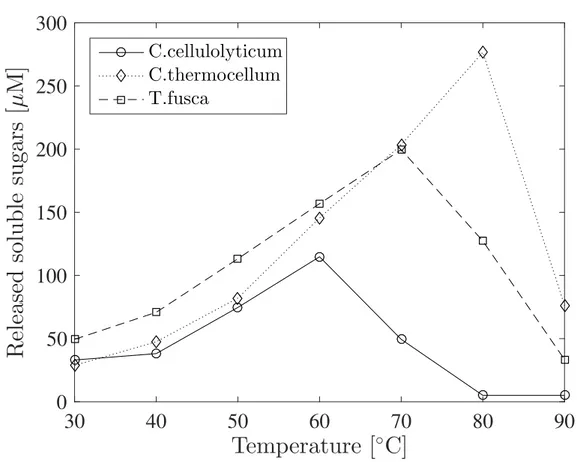
1.1 The temperature dependence in the activities of three homologous proteins, Cel9 cellulases. The protein cellulase is an enzyme that helps the glycolysis of the complex sugar molecule cellulose into monosac-charides. These enzymes come from three different bacteria which live at three different optimal temperature: the Clostridium cellulolyticum, the Thermobifida fusca and the Clostridium thermocellum. In the graph it can be seen at different temperature the quantity of released sugars, the product of the reaction that this protein enhances, assayed after the same amount of time and the same conditions for each one. The data plotted in this figure is taken from [27]. . . 5
2.1 The schematic representation of the Könisberg’s bridges problem. . . 22
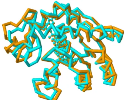
3.1 Example of two aligned proteins in Glyakina database: two C-phycocyanin proteins, with PDB ID 1KTP for the thermophilic and 1JBO for the mesophilic.. . . 34
3.2 Example of two aligned proteins: two homologous Adenylate Kinase whose PDB IDs are 1ZIP for the thermophilic protein and 1P3J for the mesophilic one. . . 36
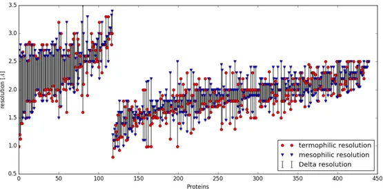
3.3 The resolution of all the couples in the database. The bars connect each thermophilic protein’s resolution to its mesophilic counterpart. The first 133 pairs are the ones that have at least one protein with resolution over the chosen threshold of 2.5 Å, while the others are the better ones. . . 38
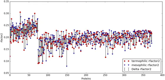
3.4 R-factor of each protein in the database. The bars indicate how much the R-factor of the two proteins in every couple is distant from each other. The first 85 pairs are the ones that have at least one protein with R-factor over the limiting threshold of 0.23, followed by the good ones. 67 couples are missing because their files do not contain information about the R-factor of their model. . . 39
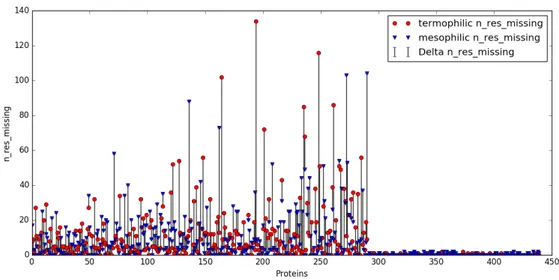
3.5 For each couple it is shown the number of missing residues for the termophilic and the homologous mesophilic protein. The first 304 couples have more than 1 missing residue; 89 of the others have 0 missing residues. . . 40
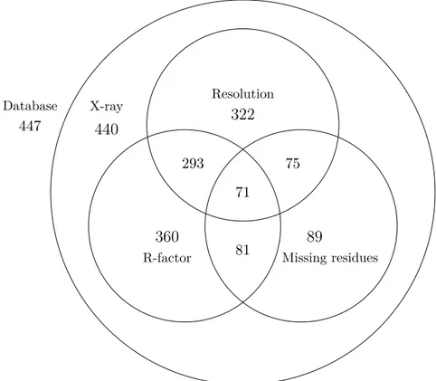
3.6 The number of pairs that remained in the database after the quality check on the PDB files. . . 41
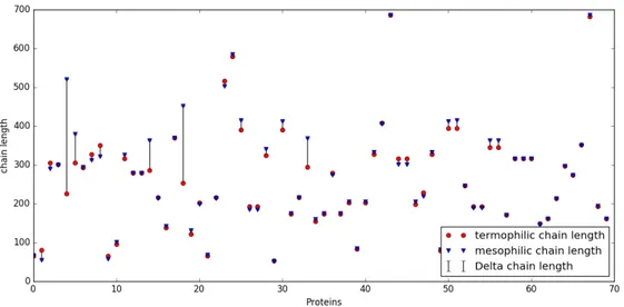
3.7 The length of each protein chain in the database. The bars highlight the difference between the thermophilic protein and its mesophilic homologous. . . 42
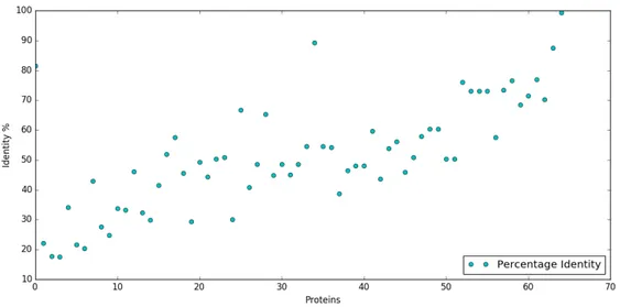
3.8 Percentage Identity of each pair of proteins in the database. . . 43
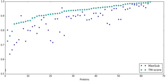
3.9 The graph shows the coefficients MaxSub and TM-score of every couple of proteins in the database.. . . 44
3.10 The value of d0 for the MaxSub and TM-score at different values of
N, the length of the target protein. . . 45
4.1 Distance matrices for a couple of rubredoxin, the thermophilic from Pytococcus furiosus (PDB ID: 1caa.A) on the left and the mesophilic from Desulfovibrio vulgaris (PDB ID: 8rxn.A) on the right. . . . 51
4.2 Distance histograms of the dataset for the various kind of distance matrices. . . 53
4.3 Protein contact maps for a couple of rubredoxin, the thermophilic from Pytococcus furiosus (PDB ID: 1caa.A) on the left and the mesophilic from Desulfovibrio vulgaris (PDB ID: 8rxn.A) on the right. The colors represent different threshold choices, as specified in their color bar.. . 55
4.4 Frequency of having a contact vs. the distance in the primary structure of the two residues, i.e. the diagonal number of the cell in the PCM, for the first 50 positions. . . 56
4.5 Distribution of the CO and LRCO values of the Cβ and closest atoms maps. . . 58
4.6 The eigenvalues of the closest atoms contact map Laplacian and normalised Laplacian for the couple of proteins 1caa.A and 8rxn.A. . 60
4.7 The first eigenvalues of the Laplacian on the left and of the normalised Laplacian on the right, plotted thermophilic vs mesophilic. . . . 61
4.8 The last eigenvalues of the Laplacian on the left and of the normalised Laplacian on the right, plotted thermophilic vs mesophilic. . . . 62
4.9 The percentage of pairs whose sum of the first or last ten Laplacian eigenvalues is higher for the thermophilic.. . . 63
4.10 Histogram showing the distributions of the values < 1.0 of ∆s of the thermophilic and mesophilic proteins for the various type of contact map. The x axis has been limited between [0,1] to zoom in on the initial distribution. . . 64
4.12 The times each amino acid presents a high value of ∆s in the database, divided by the number of times that amino acid is present in the database. 66
4.13 Occurrences of substitutions in the database for residues in the mesophilic proteins with high values of ∆s for Cα and Cβ contact maps, normalized by lines. The maps on the left have been weighted with the magnitude of the ∆s of the thermophilic residue. . . . 68
4.14 Occurrences of substitutions in the database for residues in the mesophilic proteins with high values of ∆s for center of mass and closest atoms contact maps, normalized by lines. The maps on the left have been weighted with the magnitude of the ∆s of the thermophilic residue. . . 69
List of Tables
1.1 Classification of all the 20 amino acids based on the properties of their side chain. . . 2
4.1 The Van der Waals radii used for the creation of the closest atom distance matrix, taken form [1]. . . 50
4.2 The differences between thermophilic and mesophilic maps in the number of occurrences of the residues with the highest ∆s divided by the lower of the two values. In the map column the kind of contact map is indicated; CM is an abbreviation for center of mass and CA for closest atoms. . . 67
A.1 All the 894 PDB IDs of the proteins considered for the creation of the database: the list from Glyakina et al. [19], the list from Taylor and Vaisman [42] and the other couples found in literature, whose more detailed information can be found in the next table A.2. For every couple, the first one is the ID of the thermophilic protein followed by the chain , followed by the mesophilic. . . 81
A.2 In the table sixteen pairs of proteins are listed. Letters T/M indicate whether the protein is thermophilic (T) or mesofilic (M). The parame-ters Identity and Similarity are referring to the results obtained by the jFATCAT alignment tool on the PDB website[4]. . . 83
B.1 The list of the couples of proteins in the final database. The letters T/M indicate whether it is a thermophilic or mesophilic protein. . . . 92
1
Protein structure and temperature
In this chapter some background is given about how different proteins behave across different temperature ranges and why it is interesting to find proteins that keep their functionality intact at extreme temperatures. Firstly a brief description of the structure of a generic protein will be given, followed by a brief summary of the known strategies that proteins adapt in order to survive high temperatures whilst maintaining their structure intact. Most of the content from these sections is informed by the textbook Cambell Biology, ninth edition [33]. The final section discusses the techniques that are used to obtain a three-dimensional model of a protein and provide a description of the Protein Data Bank archive from which the structures used in this thesis were taken from.
1.1
What is a protein
Proteins are essential for life as we know it; almost all the dynamic functions that take place within a living being depend on proteins. In particular, life would not be possible without enzymes that speed up chemical reactions. Most of the enzymes in living organisms are proteins, working as catalysts. In nature there is a huge number of various proteins; humans have tens of thousands different variants. However, every protein consists of a specific sequence of the same twenty amino acids. Amino acids link together with peptide bonds, forming a chain. After the amino acids lose an H2O molecule to create the peptide bond, they are defined as residue. Proteins are
made of one or more amino acid polymers, named polypeptides. The polypeptides are called protein when they are folded into a three-dimensional structure. The folding and coiling of the protein is generally spontaneous under normal cellular conditions. The bonds formed between different parts of the chain, that define the final shape of the protein, depend on its particular amino acid sequence. That said, there is a great
1 – Protein structure and temperature
deal of research interest around how the amino acid chain transitions to a protein via a series of intermediate states: the protein folding. The functionality of the protein is defined by its structure which ultimately determines how it interacts with other molecules or macromolecules. But before we getting there, we must first consider in more detail the fundamental building blocks of a protein: the amino acids.
1.1.1
Amino acids
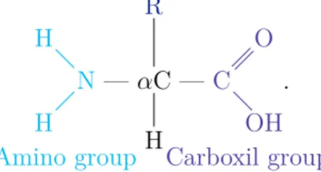
Proteins are ordinate chains of amino acids that fold into a three dimensional structure. Each of the twenty different amino acids has the same basic structure: an amino group and a carboxyl group, held together by a carbon atom, called the αcarbon. The other two links of the α carbon are made with a side chain R, which is the part that differentiate one amino acid from the others, and with an hydrogen atom. The schematic representation of a amino acid monomers is shown below:
N H H Amino group — αC H R — C O OH Carboxil group .
The side chain varies significantly for different amino acids. It can be as subtle as the displacement of a single hydrogen atom, as is the case of the smallest amino acid possible Glycine that is the only amino acid that does not have a β carbon, or as complex as a carbon skeleton with other functional groups attached, as in the one of Glutamine. The physical and chemical properties of the groupR determines the properties and the functional roles of a particular amino acid. We can classify each amino acid depending on these properties, as shown in table 1.1.
Hydrophobic Hydrophilic
Non polar Polar Electrically charged Basic, positively charged Glycine Alanine Valine Serine Threonine Cysteine Lysine Arginine Histidine (Gly or G) (Ala or A) (Val or V) (Ser or S) (Thr or T) (Cys or C) (Lys or K) (arg or R) (His or H)
Acidic, negatively charged Leucine Isoleucine Methionine Tyrosine Asparagine Glutamine Aspartic acid Glutamic acid (Leu or L) (Ile or I) (Met or M) (Tyr or Y) (Asn or N) (Gln or Q) (Asp or D) (Glu or E) Phenylalanine Trypyophan Proline
(Phe or F) (Trip or W) (Pro or P)
Table 1.1: Classification of all the 20 amino acids based on the properties of their side chain.
The various amino acids connect together in sequence, by means of the peptide bonds. Peptide bonds are formed as a result of dehydration synthesis, where a
1.1 – What is a protein
covalent bond is created by removing a water molecule from the carboxyl group of one amino acid and the amino group of the other, as shown by the following schematic reaction: C O OH Carboxyl group (C-terminus) + N H H Amino group (N-terminus) C O N H Peptide bond + H2O Water
These concatenations of amino acids are polymers called peptides – or polypeptides when they are formed by numerous residues. Peptides, unless they are cyclic, have two terminals: an amino end, said N-terminus, and a carboxyl one, called C-terminus.
The linear order of amino acids in the peptide, which determines the chemical properties of the molecule, is specific and unique for each one. The first protein to have its amino acid sequenced was the insulin hormone in the early 1950s, thanks to the work of Frederick Sanger [36]. He and his team worked over 12 years before determining the sequence. Prior to this breakthrough, it was only possible to measure with a certain precision the relative quantities of amino acids within a protein, without any sense of how they were arranged. Nowadays protein sequencing is an automated process and there are various methods to perform it. One process is the Edman
degradation. In this method the N-terminus of the protein is labelled and detached
form the chain without breaking other peptide bonds. By repeating this reaction, one can learn the amino acid order of the protein. An indirect way to discern the sequence of a protein, is by sequencing the gene that produces it. If the genetic material that codes for the protein is known, this is actually easier than obtaining the sequence from the protein itself.
Learning the order of the amino acids composing a polypeptide is important, but it is not sufficient to discern the properties of the final protein. That is why knowing the three-dimensional structure is crucial for the study of a protein.
1.1.2
Protein structure
The shape of a protein is the result of interactions and bonds that take place between its the components. This bonds can be seen as belonging to different structure orders. The primary structure is the linear chain of residues, that, as we have already seen, are held together by peptide bonds. This primary structure is quite far from the shape of the final protein. When a cell synthesizes a polypeptide, it folds itself helped by specialized proteins called chaperones, firstly by assuming a secondary
structureand then compacting into a tertiary one. An additional quaternary structure
1 – Protein structure and temperature
The secondary structure is composed by coils and foils; both of these structures are the result of hydrogen bonds between backbone oxygens and amide hydrogens. Coiled parts are called α-helix, structures that are held together by hydrogen bonding between every forth residues. A protein can have more α-helices spaced out by flat regions. The other regular secondary structure is the β-pleated sheet, or simply β-sheet. In this case two or more strands of the polypeptide, the β-strands, typically composed of 3 to 10 amino acids, are lying in parallel. This formation is kept together by a wide network of hydrogen bonds between neighbours.
The tertiary structure is superimposed to the secondary one. The main difference between the secondary and the tertiary structure is that, while the first is realized by hydrogen bonds between the backbone elements, the second is the result of interactions between the various side chains. In fact, hydrogen bonds are considered belonging to the tertiary structure when they are connecting hydrophilic side chains, but there are more types of interactions that can occur at this level. One is the hydrophobic interaction. This interaction is obtained by the spontaneous formation of clusters of hydrophobic side chains in the core of the protein, repelling the contact with water, and the stability of these clusters is increased by the formation of Van der Waals interactions between these non-polar R groups. Another kind of bonds that can occur at this level are ionic bonds between opposite charged side chains. Furthermore, also part of the secondary structure are disulphide bridges (–S–S–) that can form between two cysteines that happen to have their sulfhydryl groups (–SH) near each other, further reinforcing the stability of the protein.
In addition to these three structure levels – primary, secondary and tertiary – that are always present, there can be also a quaternary one. The quaternary structure is the overall functional macromolecule that is the result of an aggregation of more than one polypeptide chain. A well known example of this structure is haemoglobin, that consists of four polypeptide subunits.
Every protein has its own structure and interestingly enough there are also proteins that present functional parts that remain unfolded. Since the structure of the protein is formed by interactions between its components, it can be jeopardized when those bondings are put under stress, like in the case of high thermal agitation.
1.2
Structure and temperature
Many factors of the environment where the protein is affect its structure and, accordingly, its functionality. In particular temperature, pH and pressure have major consequences on the protein structure and on how efficiently it works. Each protein has its optimal conditions, that is when its most active shape is favoured.
With regards to the temperature, the functionality of a protein changes quite rapidly. Initially, as the temperature rises so does the activity of the protein. Then, above a certain threshold, which is considered the optimal temperature for that
1.2 – Structure and temperature
30
40
50
60
70
80
90
Temperature [
◦C]
0
50
100
150
200
250
300
R
el
ea
se
d
so
lu
b
le
su
ga
rs
[µ
M
]
C.cellulolyticumC.thermocellum T.fuscaFigure 1.1: The temperature dependence in the activities of three homologous proteins, Cel9 cellulases. The protein cellulase is an enzyme that helps the glycolysis of the complex sugar molecule cellulose into monosaccharides. These enzymes come from three different bacteria which live at three different optimal temperature: the
Clostridium cellulolyticum, the Thermobifida fusca and the Clostridium thermocellum.
In the graph it can be seen at different temperature the quantity of released sugars, the product of the reaction that this protein enhances, assayed after the same amount of time and the same conditions for each one. The data plotted in this figure is taken from [27].
protein, the activity declines. An example of these curves is shown in figure 1.1, where three homologous enzymes, i.e. that perform the same task in three different organisms, have different optimal temperatures. The trend of those curves is due to thermal agitation. As a matter of fact, thermal agitation augment the probability of collision between the active site of the protein and the substrates, accelerating the reaction, but this is true only up to a certain temperature, the optimal one for that enzyme, at which the enzyme is the most active. After that, a further increase in temperature results in the break of bonds that stabilise the active structure of the protein, lowering its functionality and eventually causing its denaturation. A protein is said to denature when the disruption of its structure causes the loss of its
1 – Protein structure and temperature
functionality.
It is clear that every protein has its own optimal temperature. Out of the window of temperatures where the structure is solid enough to maintain its active sites stable, but at the same time flexible enough to be able to interact with the substrates, the protein can not perform its task. Since cellular life depends on protein activities, major damages, that can lead to the death of the organism, arise when proteins are out of their temperature range. Most of the cells, human ones comprised, live at temperatures between 35◦C and 40◦C. Complex organisms, instead, can survive out
of their preferred interval if they are able to spend energy to keep their cells within the right temperatures, as in the case of mammals and birds. Organisms that live at these temperatures are called mesophiles (which literally means who loves the middle, and it is composed by the Greek words μέσος, middle, and φιλία, love). There are, however, other organisms that thrive at other temperature ranges thanks to some extraordinary adaptations. They are part of a group called extremophiles (literally meaning who loves extreme conditions, from the Latin extremus), and they can be classified into two types:
• the thermophiles (who loves the heat, from the Greek θερμότητα, heat), who thrive at temperatures between 41◦C and 122◦C – if their growth temperature
is higher than 85◦C they are called hyperthermophiles and interestingly many
of them can not even reproduce themselves at temperature below 80◦C;
• the psychrophile or cryophiles (who loves the cold, from the Greek ψυχρός or κρύος, cold), who live at temperature between 20◦C and −10◦C Celsius.
In nature other types of extremophiles exist. As an example, there are organisms that can survive high salt concentrations or extreme pH values. Anyway, they fall outside the aim of this thesis and so they will not be considered here.
1.2.1
Interest and utility of extremophilic enzymes:
the
PCR example
Apart from the obvious academic interest and the intellectual curiosity in life forms that have inhospitable places, such as hot springs or brine pockets surrounded by sea ice, as their habitats, there are other good reasons to study them. The extremophiles indeed express enzymes that can be operative at “extreme” optimal temperatures. These enzymes are hence called extremozymes. They can be used for pharmaceutical, industrial and for research purposes in reactions at not standard temperatures. One of the possibly most significant example of such usage is the
Polimerase Chain Reaction technique, commonly referred to with its acronym PCR.
PCR was developed in 1983 by Kery Mullis, although a very similar idea was firstly introduced in 1971 by the Norwegian Kjell Kleppe [22]. This method won
1.2 – Structure and temperature
Mullis a Nobel Prize for Chemistry in 1993. It is thanks to this technique that scientists have been able to isolate and study the DNA of HIV and to analyse genetic materials from very scarce sources, like fossils or dried blood on crime scenes. The method itself is quite simple and it allows to replicate in a test tube a single DNA segment, obtaining billions of copies in a few hours [29]. This multiplication is made by an enzyme, the DNA polymerase, that copies a single strand of DNA when a
primer, i.e. a small amount of complementary bases, is already attached to the
starting point on the original strand. In order to have a single DNA strand the DNA’s double helix has to be melted, which means that the hydrogen bonds connecting complementary bases have to be broken. This is obtained by heating the DNA at 94 –98◦C. Then there is the annealing step, which occurs at a lower temperature,
where the primers bind with the initial part of the genetic code which needs to be copied. At this point everything is ready for the DNA polimerase to perform its task, doubling the initial amount of DNA. This cycle has to be repeated in order to have the desired number of DNA strands, usually something around 20-30 times, getting ∼220−30 '106−109 pieces of the same DNA.
Initially, they used the enzyme DNA polymerase I form Escherichia Coli, which works well at 30◦C but denatures at the high temperatures required to melt the DNA.
This forced the researchers to add this enzyme at every cycle after denaturation and it was difficult to achieve an automated procedure. What Mullis himself said to be “one of the most important improvements in the process” [30] was the introduction of an enzyme extracted from another organism, the thermophilic Thermus Acquaticus, that has its peak of activity around 75◦C-80◦C [23]. The major advantage was to
have an enzyme that could survive long incubation periods even at 95◦C, and so
it only needed to be added at the beginning of the reaction, making it possible to be automated. What is more, it also improved the performance of this technique because it produced an increase in specificity, yield and sensitivity of the process [35]. Nowadays also other DNA polymerases are used [39]. An example is the one extracted from the termophilic organism Pyrococcus Furiosus, which is more accurate. In fact it has an error rate in the order of 10−6 and the copies contain less than 10% of the
mutations caused by the Thermus Acquaticus’s enzyme [25].
1.2.2
The extremophiles and their evolution
Ascertained that it is worth studying the extremophiles, and in particular their proteins, it seems crucial to try to understand how they can survive in their impossible, from an anthropocentric view, habitats. Thermophiles have been able to adapt to high temperatures, so their enzymes are likely to have optimal temperatures at higher points than mesophilic ones. In fact, due to the little dimension of the thermophilic cells – in the scale of the micrometer – insulation from the hot environment appears impossible; therefore the cell components, including its proteins, have to be heat
1 – Protein structure and temperature
resistant [40]. This is possible thanks to their firmer structure, which is less prone to disaggregate because of thermal agitation. Psychrophile, on the other hand, have evolved to survive even below 0◦C, but still the point of water freezing in cells
remains a lower limit for life – with the exception of the nematode Panagrolaimus
davidi, that can survive water freezing in its body. The littler thermal agitation in
this case makes the contact between substrates and proteins less probable, causing the activity to be consistently lower then a mesophilic homologous. This is the reason why their enzymes have to be very efficient in order to produce enough product at life-compatible time rate.
So, how is it possible for extremozymes to function in those conditions? Since in this thesis we are going to compare thermophilic proteins to mesophilic ones, it will follow a discussion about the adaptations of organisms that thrives at high temperatures. There are various micro-organisms with this ability, and can be either bacteria – like photosynthetic bacteria, enterobacteria and thionic bacteria – or, as it happens for the majority of known thermophiles, archaebacteria – like Pyrococcus or Thermoccocus. According to Morozkina et al.[28], in 2010 more than 70 species, 29 genera, and 10 orders of thermophiles were known, but still the matter about the origins of these life forms is not totally resolved. On the one hand it seems that, from phylogenetic studies 1 , the thermophiles should have appeared at the time of the
origin of life itself on Earth, preceding the mesophiles. On the other, some authors still prefer the hypothesis which sustain that the thermophiles descended from the mesophiles organisms, as a consequence of adaptation to high temperature [28]. It is anyway possible that both these things happened, and some thermophiles are the result of a mesophile colonizing – or recolonizing – an hot environment while others directly originated in the extreme habitat [3].
1.2.3
Extremozymes adapted to hot habitats
The problem of the extraordinary thermal stability of thermophiles has been the subject of studies since they were discovered. It was found that there are different ways they adapted themselves for living in their extreme habitats. For example, differences have been found between thermophilic archea and thermophilic bacteria in the type of membrane lipids [28].
With respect to the stability of the protein structures, a certain variability of adaptations has developed, potentially connected to the evolutionary history of
1The phylogenetic studies were carried on characterising some genes in the ribosomal RNA, to
be precise the 16S, in prokaryotes, and the 18S, in eukaryotes, rRNA genes. The choice of this particular segment of the genetic material present in every cells, is due the fact that are essential components of the cell, and so one can find them in all self-replicating systems, and that their sequence changes slowly with time, allowing to relate very distant species [47].
1.2 – Structure and temperature
the expressing organism. It is suggested that if the organism had originated in the hot environment it would prefer “structure-based” mechanisms of adaptations, presenting more compact and more hydrophobic proteins; if instead the organism had a mesophile ancestor it would use a “sequence-based” one, resulting in proteins with similar structures but with stronger interactions [3]. Both methods are made possible by many strategies, the most recurring are here listed.
Amino acid composition There are some more labile amino acids that are more
likely to undergo modifications at high temperatures, and therefore their half lives are shorter in those conditions. In fact, applying temperatures beyond 100°C, the thermal stabilities of the common amino acids are (Val,Leu)> Ile> Tyr> Lys> His> Met> Thr> Ser> Trp> (Asp,Glu,Arg,Cys) [34]. As a consequence in thermophilic proteins, compared to mesophiles homologous, there are less residues that are particularly thermolabile, such as asparagine, cysteine, glutamic acid and aspartic acid [10]. What is more, some other changes in the amino acid composition may lead to a more robust protein. As an example, Van den Burg et al.[43] operating some “rigidifying” mutation – such as glycine and alanine been replaced, respectively, by alanine and glycine in delicate regions of the protein – to a relatively thermostable enzyme, managed to have a hyperstable one. Furthermore, it seems that charged residues are preferred [3], increasing the possibility of having a stronger ionic network.
Ionic networks The study of thermophilic protein structures indicates that ion
pairs on the surface of subunits and domains may be important for their stability. In fact, networks of ionic interaction have a longer range than hydrophobic ones and do not depend on the alteration that water undergoes at high temperature. On hyperthermophilic proteins, more extensive ionic networks, spatially alternating of positive and negative charges, have been observed than on thermophilic or mesophilic counterparts [10] [34]. An interesting study by Vetriani et al.[44] showed how subtle changes in the amino acid sequence of a protein, made in order to reinforce its ionic network, result in major changes in its thermostability. They substituted only two bases in the hexameric glutamate dehydrogenases from Thermococcus litoralis and, although the single swings proved to have an adverse effect on thermostability, together they protracted of almost 4-times the half life of the protein at 104◦C. Hydrophobic packing Notwithstanding the fact that many amino acids are more
stable when they are inside a hydrophobic packing, it is still not clear what is the temperature role in the strength of hydrophobic interactions. It is not certain whether at higher temperatures they become stronger or weaker. In any case, it is a common feature of stable globular protein to have a closely packed hydrophobic core [34].
1 – Protein structure and temperature
Cooperative association It has been observed that sometimes the structure of a
thermophilic oligomer, i.e. a protein complex made of two or more subunits, can be more elaborated than its mesophilic homologous, that could even consists of just a monomer. This is due to the denaturation of monomers that follows the dissociation of the oligomer. Therefore, thanks to strong inter-molecular forces, the process of the unfolding is forestall [10] [34].
A compact structure Some thermophilic proteins present a more compact
struc-ture compared to mesophilic ones. A common alteration concerns the α-helixes to β-layers ratio [10]. Preferring for their secondary structure the more packed β-layer, extrmozymes have less cavities and a lowered area to volume ratio. Another strategy consist of preclude N– and C– termini’s movements. Preventing the loose ends from fraying stabilizes the structure, limiting the chances of unraveling. This can be obtained in different ways, for example keeping the termini in hydrophobic pockets, substituting disordered loops with α-helix structures or using ion-pairing [34].
1.3
Studying the structure of a protein
It is now well clear how important the protein structure is: from the three-dimensional disposition of its residues descends a number of properties, like the very function of the protein and the temperature range in which the function is active. As a consequence, being able to understand and study the three-dimensional assemblage of the various proteins is crucial. So far, two main methods for experimentally obtaining them have been used:
• X-ray crystallography;
• Nuclear Magnetic Resonance (NMR) spectroscopy.
To these two, Bioinformatics is to be added, a newer approach that does not need a direct observation of the folded protein, but relies only on the predictions that softwares can make from the linear sequence of the amino acids. Even if the predictions can be quite accurate, the protein folding problem is still not resolved, so this last method is mainly used as a complementary approach in understanding protein structure.
All the protein structures examined in this thesis were obtained with X-ray crystallography. As a matter of fact, while the two methods usually model structures with the same backbone topology, they often produce different local features, like for example surface loops [48]. This is caused by the different samples used for these techniques. In the NMR spectroscopy case, highly purified proteins are dissolved in an aqueous solution, while for the X-ray crystallography, as the name suggests, the sample consists of a solid protein crystal. This is one of the reasons why X-ray
1.3 – Studying the structure of a protein
crystallography yields to higher resolution results, which is ultimately the cause of the choice of using only structures obtained this technique.
In the next section we are going to explain how protein X-ray crystallography works.
1.3.1
Protein X-ray crystallography
Determining the correct three-dimensional protein structure is not an easy task. The atoms in a single molecule are thousands, and finding the exact position of each of them is not simple. The first structures (of haemoglobin and a related protein) were obtained in 1959 with X-ray crystallography. This achievement was attained many years after this technique was born with the first pioneering studies on simple inorganic crystals by Max von Laue in 1912 and by Bragg father and son in the following years.
X-ray crystallography is possible tanks to the regularity of crystals and the wave proprieties of the electromagnetic radiation. An X-ray beam striking an electron makes it oscillate at the same frequency of the original beam. An oscillating electron emits a spherical wave with the same frequency as the incident one. This phenomenon is called elastic scattering. From the analysis of the scattered light wave it is possible to resolve the electron density of the crystal. This wave is “simply” the sum of all the scattered waves by all the electrons in the crystal. The periodicity of the crystal makes it possible to go from the scattered pattern to the electron density distribution.
For understanding what happens when there is a diffraction we follow the approach presented in Principles of Protein X-Ray Crystallography, by Jan Drenth [14]; so we start considering the scattering from a couple of electrons, the first one in the origin of our frame of reference and the other in ~r. We consider an incident X-ray wave with wave vector | ~k0|= 2π/λ and the diffracted light with wave vector ~k, which
has the same magnitude of the incident one thanks to the fact that the scattering is elastic. The amplitude A of the wave scattered from the first electron is the same of that from the second, but there is a difference in the phase. This is caused by a difference in the light path of ~r · ~k0λ/(2π) − ~r · ~k λ/(2π), which results in a
phase difference of ~r · (~k − ~k0) = ~r · ~q, where |~q | = 2 sin ϑ (2π)/λ, with ϑ being the
incident angle of the primary wave with an imaginary reflecting plane. This leads, thanks to the adding property of electromagnetic waves, to a total scattered wave of
A[1 + exp(i~r · ~q)]. Supposing now to shift the origin of the system of − ~R, so that
the first electron is now in ~R and the second one is in ~R + ~r, following the previous line of reasoning, another phase displacement of exp(i ~R · ~q) has to be added to both the waves, resulting in a scattered wave with the same amplitude:
1 – Protein structure and temperature
Let us now consider an atom and its electron cloud with %(~r) density. We have now the origin of the reference frame in the nucleus, since a displacement would only result in a phase shift common to all electrons as just seen. The amount of scattered light depends on the number of electrons and their position in the cloud, so the atomic scattering factor f is defined as:
f(~q) = Z
V
%(~r)ei~r·~qd~r. (1.2)
The atomic scattering factor can be looked up in tables, where f is expressed as a function of the module of ~q, as the electron cloud of an atom is assumed spherically symmetric and so the direction of ~q is irrelevant. What is more, f, which is actually the Fourier transform of the electron density map, is always real thanks to this symmetry of the cloud. From the single atoms we now move on considering a unit cell. The scattering of the unit cell is nothing but the sum of the scattering from the single atoms that compose it. Since the nucleus of the j–th atom is not centred in the origin of the system, but it is now in ~rj, a phase angle of ~r · ~q must be added to
the atomic scattering factor fj. The structure factor F (~q) is then defined as:
F(~q) =
n
X
j=1
fjei~rj·~q. (1.3)
The last step consist in considering the whole crystal. Suppose that the crystal has n1 cells in direction ~a, n2 in direction ~b and n3 in direction ~c, being ~a, ~b and ~c
the translation vectors of the crystal. Then the total scattering factor is:
K(~q) = F (~q) × n1 X s=0 eis~a·~q× n2 X u=0 eiu~b·~q× n3 X v=0 eiv~c·~q. (1.4)
But since the number of cells in every direction is a very high one, Pn1
s=0exp(is~a · ~q)
would be almost equal to zero, unless ~a · ~q = 2πh, with h integer, and so on for the other translation vectors. Hence follow the Laue conditions:
~a · ~q= 2πh, h ∈ Z ~b · ~q = 2πl, l ∈ Z ~c · ~q = 2πk, k ∈ Z. (1.5) From these equation it appears clear that it is crucial to have a good periodicity in the crystal in order to be able to analyse the data. Unfortunately obtaining a suitable single protein crystal is the least understood step in the whole process, so it is mainly a trial-and-error procedure that leads to the precipitation of the protein form its solution. The purity of the protein is surely an important factor. In fact, compound other then the protein itself should be absent and also all the molecules in the protein should present the same surface properties. The crystallization of protein is obtained in four steps:
1.3 – Studying the structure of a protein
1. The protein’s purity has to be determined (e.g. with a mass spectrometry). If it is not satisfactory, further purification will be necessary.
2. The protein is dissolved in a solvent, which is usually a water-buffer solution. Membrane proteins that are insoluble in such solvent require the addition of a detergent.
3. The solution is then brought to supersaturation. During this step little aggre-gates are formed. Those aggregations will become the nuclei for the growth of the crystal. Precipitation of the protein is achieved in more then one way, like changing the pH or the temperature, or, one of the most common method, increasing the concentration of the protein by adding a salt (salt-out) or polyethyleneglycol (PEG) to the solution.
4. After the formation of the nuclei, the actual crystal growth begins. More molecules or other small nuclei get attached to the starting nuclei, forming the crystal. This step is quite critical. One of the reason is that, if the supersaturation is too high, too many nuclei are formed resulting in many small crystals. So it is important to have a lower level of supersaturation then in the previous step. What is more the optimal growth process is a very slow one to achieve a high order degree, so it would be better to not change the temperature as a way to modify the supersaturation.
Once a pure enough and big enough (usually 0.3 mm × 0.3 mm × 0.3 mm, approx-imately 15 µg) crystal is obtained, it is exposed to an X-ray diffraction trial. To do so, the crystal has to be mounted on an appropriate support. Usually two roads can be taken: putting it in a capillary test tube at or near room temperature or suspend it in a small loop in a stream of liquid nitrogen at a temperature range of 100 K to 120 K. In the first case the crystal is pushed carefully in an air gap between two layers of mother liquor, i.e. the solvent used to precipitate the proteins. It is very important to not change the environment of the crystal, because the spherical or egg-shaped macromolecules are loosely packed in the crystal, surrounded by the solvent that fills the gaps between them, so any loss of the mother liquor destabilizes the crystal. The second option has the advantage of the low temperature in maintaining the crystal structure. In fact, the very exposure to the X-ray radiation damages the crystal and the diffraction pattern dies after a few hours at room temperature. Nevertheless, the cooling of the crystal has to be treated very carefully. It has to occur suddenly, hence the names of the technique flash freezing or shock cooling, because the mother liquor in the crystal must freeze to a vitreous substance and not crystallize, otherwise ice crystals would damage the protein crystal structure.
The diffraction pattern is then acquired. Different X-ray sources and detectors can be used for this goal. Very briefly, as this could lead us far form the aim of
1 – Protein structure and temperature
describing protein crystallography, it is possible to obtain an X-ray beam from three different sources:
Sealed or rotating anode tubes Both of these tubes have at their base the same
functioning idea: a cathode emits an electron beam, the electrons accelerate towards the anode and collide with it at high speed. Most of the energy of the impact is converted to heat, that has to be removed by cooling the anode, usually with water, in the case of the sealed tube, or by rotating it, as the name suggests this is the case of a rotating anode tube, in order to change the place of impact and give it time to cool down before being hit again. However, a part of the energy is emitted as X-rays thanks to the interaction between the electrons and the anode material. The spectrum of the X-ray emitted presents a smooth continuous region, called the “Bremsstrahlung” radiation, that is radiation emitted due to the deceleration of the charged particles, electrons in this case, and sharp peaks called characteristic radiation, emitted by electrons of outer shells lowering their energy level in order to take the place of K-shell electrons ejected after a collision with a fast moving electron coming from the cathode.
Particle accelerators Synchrotron radiation is obtained from a particle accelerator,
a big and expensive facility. Charged particles, as electrons or positrons, are accelerated and injected into the storage ring where they circulate. Every time the particle beam changes direction, having its path bended by a magnet, it accelerates and some radiation is emitted. This lost in energy is compensated for with radiofrequency input at every cycle, and when the first synchrotrons were built it was considered an annoying wast of energy, being their primary objective to obtain high energy particles’ collisions. Anyhow nowadays synchrotron radiation is very interesting for various applications and experiments since the quality of the X-ray beam is higher than that of a ordinary X-ray tube. The intensity of the synchrotron light beam obtained is up to two orders higher, the beam has a low divergence, a monochromator can select any suitable wavelength in the spectral range and the light is polarized.
To collect the diffracted light, single photon counters were used since the early years of X-ray crystallography, but they, although very precise, have the big disadvantages that it takes several weeks to obtain a complete data set for one protein. Photographic film was a good alternative, with a resolution superior than modern day detectors, but the process of developing the film is quite time consuming as well and it has a limited dynamic range, making necessary to use three consecutive films when the full X-ray intensities’ range was needed. A first alternative is using a image plate. Image plates have a higher sensibility and dynamic range than photographic films. Image plates have to be read after the exposure to the X-rays, since they retain energy, proportional to the number of photons that hit that area, that can be released on
1.3 – Studying the structure of a protein
illumination with light. More convenient are area detectors that can process the signal immediately after the detection. They can be gas-filled ionization chambers or semiconductor detectors.
Once the diffraction patterns, for various crystal orientations, are collected, it is time to do some data analysis and convert it into an electron density map. The data set usually consist of hundreds of single two-dimensional images that have to be merged, that is identifying the same peaks in different images, and scaled in order to have the same intensity scale. The data is a representation in the reciprocal space - the reciprocal lattice is the Fourier transform of the crystal lattice written as a Bravais lattice - of the crystal lattice. It is easy to see that the total scattering factor, which is proportional to the the structure factor from equation 1.3 with the Laue conditions 1.5, is actually the Fourier transform of the electron density writing it as an integration on the all cell volume:
F(~q) = Z cell %(~r)ei~r·~qdV = V 1 Z x=0 1 Z y=0 1 Z z=0
%(x, y, z)ei[~ax+~by+~cz]·~qdxdydz
= V 1 Z x=0 1 Z y=0 1 Z z=0
%(x, y, z)ei2π[hx+ly+kz]dxdydz, for h, l, k ∈ Z
= F (h, l, k) = |F (h, l, k)| eiα(h,l,k), for h, l, k ∈ Z.
From this results that the electron density map can be obtained with the inverse transform, i.e. the Fourier transform of the structure factor:
%(x, y, z) = 1 V X h X l X k |F(h, l, k)| eiα(h,l,k)e−i2π[hx+ly+kz]. (1.6)
The integration has been replaced by a summation because of the Laue conditions. The reason why F (h, l, k) has been explicity separated into its module and its phase it is going to be clear soon, and it has to do with what we detect from a crystallographic experiment. In fact, the data collected from a crystallographic experiment is basically the intensity of the scattered waves, that can be written as:
I(h, l, k) = (AS)2|F(h, l, k)|2, (1.7)
where S is a proportionality constant. This now makes clear that if |F (h, l, k)| can be deduced from the experiment, the phase exp[iα(h, l, k)] can not, leading to what is called the phase problem. Fortunately several methods have been developed to have an initial guess for the phase and then iteratively perfect it while maximizing the correlation between the diffraction data and the model obtained.
1 – Protein structure and temperature
There are some parameter that one can calculate from the obtained model and the diffraction pattern that can quantify the quality of the model itself. The most important ones are here listed and described, citing as typical values the ones indicated in the relevant sections of the online portal PDB-101, at the website
rcsb.org[4].
Resolution The resolution of an electron density map depends on various things
and is a first parameter that shows the quality of the data collected. As a matter of fact, resolution tells how much detail is present in the diffraction pattern and, as a consequence, in the final model. This depend on the experimental equipment used, on the conditions of the experiment, e.g. the temperature, and on the purity and the order of the crystal. A structure that presents all its fine details, showing all its atoms on the electron density map, is said to be at high-resolution, having little resolution values around 1 Å. On the contrary, for low-resolution structures, that have resolution values of 3 Å of higher, only the basic skeleton of the protein can be seen and the atom position is inferred. The majority of the structures have a resolution in between those two peaks.
Temperature factors or B-factors If the resolution is a characteristic of the
whole model, more detail on the accurate positioning of the single atoms can be obtained with the temperature factors, also called B-factors. These values give an insight on the displacement of an atom from its mean position. The more the atom moves from its average, i.e. the more flexible it is in the protein crystal, the higher the associated B-factor. The typical values for the temperature factors are around 15-30 Å2
, with possible peaks way larger than 30 Å2
for very flexible regions. Such parts of a protein can be shown on a 3D chart representing each atom in its coordinates and adding a red color to the ones with the highest B-factors and a blue color to the ones with the lowest, B-factors in between represented by an appropriate blend that allows to see how close are to one of the extremes.
R-value and R-free value The R-value carries another important information
about the model obtained. It is a measure of how well the diffraction pattern simulated from an hypothetical crystal made with the calculated protein model compares to the experimental diffraction pattern. This provides a quantitative information about the quality of the reconstruction carried out from the empirical data. On the one hand if the two patterns overlap perfectly the R-value is 0, while on the other if the atoms of the proteins are positioned randomly the R-value is close to 0.63. These of course are extremes, whereas typical values of real cases are about 0.2. Sometimes the R-value can be utilized as a feedback for the reconstruction algorithm in order to refine the atomic model. Therefore the R-value of the final model can present a bias, for this reason one can look at the R-free value, an R-value obtained
1.3 – Studying the structure of a protein
on a 10% of the experimental data that is not used to optimise the model. A good model should have its R-value similar to the R-free value, but in any case the R-free is usually higher, with typical values around 0.25.
Once the model is refined and the obtained electron density map is satisfactory, it is usually deposited with all the additional information needed in a crystallographic database, such as the Protein Data Bank.
1.3.2
The Protein Data Bank and its files
The Protein Data Bank (PDB) [4] archive was first announced in 1971 [31]. Before the PDB was established, punched cards, one for each atom, were the only method to exchange protein structures’ coordinates; this reciprocity was active between only a few research laboratories. The establishment of the PDB, a joint operation by the Brookhaven National Laboratory and Cambridge Crystallographic Data Centre, made the data exchange possible for anyone. In 1999, the management moved from Brookhaven to the consortium called Research Collaboratory of Structural Bioinformatics (RCSB).
At present the PDB site, URL www.rcsb.org, provides the user with 116085 biological macromolecular structures and a number of tools for search the database, visualize entries and analyse them. At the moment, in the database there are more 100000 protein structures, nearly 3000 nucleic acid ones and more than 5000 protein and nucleic acid complexes. Proteins structures were mostly obtained with X-ray crystallography, only less than about 1/10 of them were obtain with NMR spectroscopy.
Each entry can be downloaded as a text file that presents the “.pdb” extension. The file contains various information about the protein and its structure, more then just its atoms’ coordinates. Therefore it is divided into sections. The following is a list of the sections you can find in a PDB file, even if not every one has all of them.
• Title; it presents the main descriptive records. • Remark; where various comments are inserted.
• Primary structure; the peptide or nucleotide linear sequence is presented. • Heterogen; in this section non-standard groups, i.e. groups that are not part of
the polymer as described in the primary structure section or are unknown/non-standard amino/nucleic acids, are described.
• Secondary structure; here the helix and β-sheet are described.
• Connectivity annotation; the existence and location of disulfide bonds or other linkages are stated in this section.
1 – Protein structure and temperature
• Miscellaneous features; it may describe proprieties in the macromolecule. • Crystallographic and coordinate transformation; it describes the
crystallo-graphic cell, the geometry of the crystallography, and the coordinate transfor-mation operators.
• Coordinate; it collects the atomic coordinate data. • Bookkeeping; final information.
The begin of every line in the file is a six letter word that defines the record stored in that line. Every file starts with the title section. The first record is the “HEADER” one, that contains the classification of the molecule in the file, the deposition date and the IDcode, an unique identifier of that entry within the PDB. Other information about that set of coordinates, of the file and of the molecule follows, e.g. if the entry is obsolete and has been substituted with new entries or the method used to resolve that structure. The lines with the record name “ATOM ”, in the coordinate section, present the atomic (x, y, z) coordinates in Angstroms for every standard amino acid (or nucleotide). This lines store the most important information about the structure
of the protein.
For a complete information about the structure of a pdb file, it is possible to refer to the available on-line documentation ( http://www.wwpdb.org/documentation/file-format-content/format33/v3.3.html).
With the data in the PDB archive you can perform a number of inquiries on the structure of the protein. This is also simplified thanks to the Python library BioPython [20]. It downloads the PDB file matching the provided PDB ID and from this it retrieves, with simple Python commands, information without the user having to search for it “manually” in all its lines.
In this thesis the three dimensional structures of the thermophilic and mesophilic proteins in the database, which will be described in chapter 3, have been reduced to 2D matrices, the Protein Contact Maps, as detailed in chapter 2. These are then analysed with a network approach and a series of measurements on them have been executed. The result of this analysis are presented in chapter 4.
2
Methods of analysis
In this chapter the methods used to analyse the proteins are presented. In particular, after some background about graph theory, it is discussed what a Protein Contact Map is and how it is possible to retrieve information about the dynamic of the protein from that network. The elements of graph theory are mainly taken from the book Graph Theory, by Reinhard Diestel [12].
2.1
Elements of graph theory
A protein contact map is a useful tool and it allows to look at the structure of a protein as a network. For this reason, we first briefly introduce the definition of network (or graph) and its mathematical description.
Graphs, as mathematical objects, made their first appearance in 1736 when Euler used them to solve the seven bridges of Könisberg problem [9]. The river Pregel was crossing the city, forming two big islands, which were connected to each other and the two sides of the city by seven bridges. The problem consisted in planning a walk through the city that would use each bridge once and only once. Euler imagined the problem as a graph, where the mainlands and the island were vertices and the bridges were links to and forth those vertices, whose schematic representation can be seen in picture2.1. It was the first time a problem was formalised in terms of nodes and links connecting the nodes, which are the two main components of every network, as illustrated in the next section.
2.1.1
Definition of graph
Euler for solving his problem used two different groups of elements, the links and the nodes, and indeed a graph G = (V, E) is defined as a couple of sets, one
2 – Methods of analysis
containing the vertices, or nodes or points, and the other the edges, or links or lines, that connect them:
V = {v1, v2, ...} (2.1)
E ⊆[V ]2 =ne(1,2) = (v1, v2), e(1,3) = (v1, v3), ...
o
(2.2) As a convention, the set of nodes of a graph is referred to as V (G) and the set of links as E(G), whatever the actual names of the subsets, and the set of the edges that have one end in the vertex vi is denoted by E(vi). A graph is said to be a
multigraph if multiple links between the same two vertices are allowed, as in the
case of the Könisberg problem. A link from and to the same node, i.e. of the type
e(i,i) = (vi, vi), is called a loop. The order |G|, or equivalently |V |, of a graph is
defined as the number of vertices in it; even though it is possible to have graphs with infinite number of nodes in this discussion only finite graphs will be considered, since proteins have a finite number of elements.
A B C D 1 2 3 4 5 6 7 Figure 2.1: The schematic representa-tion of the Könisberg’s bridges problem. From this broad definition one can devise many different
kinds of graphs. One classification separates undirect from direct graphs. A graph is said to be undirect when the order of the vertices in the edges is immaterial, namely e(i,j) =
(vi, vj) = (vj, vi) = e(j,i), so if the vertex vi is connected
to vj then vj is connected with vi. Conversely, a graph is
called direct when the edges have a directionality and the connection between vi and vj does not imply a link between
vj and vi; “one-way streets” between nodes are allowed in
this case.
Another dichotomy can then be seen between weighted and unweighted networks. Weighted networks G = (V, E, W ) have an additional information: a set of “weights” or “costs”
W = nw(i,j) = 0 if (v/ i, vj) ∈ E
o
, one for each edge.
Un-weighted ones have no such set or can be seen as a special
case of weighted graphs where all the w(i,j)= 1 if (vi, vj) ∈ E
and w(i,j) = 0 otherwise. Representing a graph
Graphs can be represented in many ways. They can be drawn as points (the vertices) connected with lines (the
edges). An example of this representation can be seen in picture 2.1, where the nodes are labelled with capital letters and the links with numbers. Alternatively, using a more mathematical approach, a graph can be seen as a matrix A called the adjacency matrix, that is unique for each graph, given an ordering choice of the
2.1 – Elements of graph theory
nodes. The general element ai,j of the adjacency matrix is defined as:
ai,j =
(
w(i,j) if (vi, vj) ∈ E
0 otherwise (2.3)
From the definition it is clear that only graphs with loops have nonzero diagonal elements and that undirect graphs result in a symmetric matrix.
As an example, using the alphabetical order shown in picture2.1, the same graph of the bridges of Könisberg could be alternatively represented as a matrix:
A= 0 2 0 1 2 0 2 1 0 2 0 1 1 1 1 0 .
Since this graph is a multigraph, the element ai,j of the matrix is weighted with
the number of bridges linking the nodes vi and vj.
2.1.2
Main proprieties of a graph and its components
After having introduced what a graph is and how to represent it, it is important to list some of the proprieties of a graph and its components. Those proprieties characterise each graph and are often used to analyse them.
The neighbourhood of a vertex vi is the set N(v) = {vj ∈ V(G)|(vi, vj) ∈ E(G)}.
A node vj is said to be a neighbour of or adjacent to vi, with i /= j, if it is in the
neighbourhood of vi. Conversely, vi and vj are said to be independent if there is no
edge between them.
The degree |E(vi)| = d(vi) = ki of a node vi is defined as:
d(vi) = N
X
j=1
ai,j,
that is the number of its neighbours if the graph is unweighted, or the sum of the weights associated with the edges that have an end in vi. A vertex whose degree
is null is called isolated. A graph whose nodes have all the same degree k is called
regular or k-regular. From the definition of the node degree, a number of proprieties
of a graph follows, like the minimum degree of a graph G δ(G) = min{ki|vi ∈ V(G)},
or the maximum degree ∆(G) = max{ki|vi ∈ V(G)} and the average degree of G
d(G) = |G|1 P
iki.
Now the definition of path will be introduced, which has always been central in network analysis since its beginning. In the case of a network of streets or transport