High-enthalpy geothermal reservoir model calibration using PEST

(1)

ALMA MATER STUDIORUM - UNIVERSITÀ DI BOLOGNA

SCUOLA DI INGEGNERIA E ARCHITETTURA

DIPARTIMENTO DI INGEGNERIA CIVILE, CHIMICA, AMBIENTALE E DEI MATERIALI CORSO DI LAUREA IN INGEGNERIA PER L’AMBIENTE E IL TERRITORIO

CURRICULUM EARTH RESOURCES ENGINEERING

TESI DI LAUREA in

Petroleum Geosystem

HIGH-ENTHALPY GEOTHERMAL RESERVOIR MODEL CALIBRATION

USING PEST

CANDIDATO RELATORE:

Silvia Armani Chiar.mo Prof. Villiam Bortolotti

CORRELATORE PhD Dr. Ester Maria Vasini

Anno Accademico 2015/2016 Sessione III

(2)

(3)

(4)

ABSTRACT

The main purpose of this thesis work is focused on the use of PEST (Parameter Estimation) to calibrate numerical models of High Enthalpy Geothermal Reservoirs (HEGR). PEST is a parameter estimation and analysis of the uncertainties of complex numerical models tool, that can be instructed to work with a standalone simulator. So, the T2Well-EWASG was used as coupled wellbore-reservoir simulator for multiphase-multicomponent HEGR. The idea of this thesis work is that the possibility to implement some automation degrees in the wellbore-reservoir model calibration task would improve substantially the Reservoir Engineers work. To become familiar with PEST, it has been necessary a preliminary training to learn how to manage its input files, its keywords, and the utility programs having the function of verifying the correctness and consistency of the created files. Then, one of the examples of PEST manual (which Fortran source code is supplied) was reproduced and analyzed, and subsequently modified. In particular, starting from this example, a simple linear model with two free parameters, some changes have been performed: "fixing" a parameter to inhibit its change during the calibration; reading a more complex model output file respect to the original example; inserting dummy data that should not be processed and instructing PEST to consider only the data of interest; changing the model adding parameters to be calibrated, and including them in the analysis changing the PEST inputs files. Finally, these skills were applied to use PEST with T2Well-EWASG to calibrate a numerical model, relative to a real HEGR, previously calibrated via a trial and error approach in a PhD thesis work. Among the real data used there were also short production-tests done in a geothermal field located in the Dominica Commonwealth.

The preliminary results show that the PEST-T2Well-EWASG calibration system works fine, and that it is a useful tool that can improve the work of reservoir engineering.

(5)

(6)

List of Figures

Figure 1. General scheme of a model calibration ... 10

Figure 2. Summary scheme that relates all the notions linked to models explained in the paragraph 1.1 and 1.2. ... 11

Figure 3. The geothermal gradient .. ... 12

Figure 4. World map showing variation in surface heat flow. ... 13

Figure 5. Different possible types of grids. ... 19

Figure 6. TOUGH2 input file example. ... 23

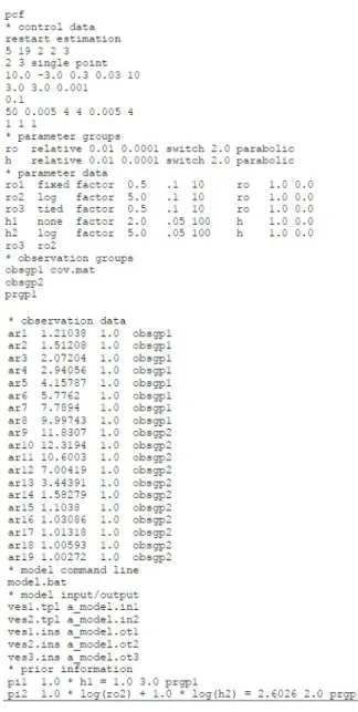
Figure 7. Example of PEST input file. ... 29

Figure 8. Example of PEST template file. ... 29

Figure 9. Example of Control file, extracted from PEST User Manual Part I, 2016. ... 40

Figure 10. Statements order that is required in a unit of a Fortran program. ... 46

Figure 11. The CodeBlocks user interface. ... 49

Figure 12. Data of file soilvol.dat fitted in two straight lines: the “residual shrinkage” segment and the “normal shrinkage” segment. ... 52

Figure 13. Two line model parameters scheme. ... 53

Figure 14. The source code of the example model. ... 54

Figure 15. in.dat input file. ... 54

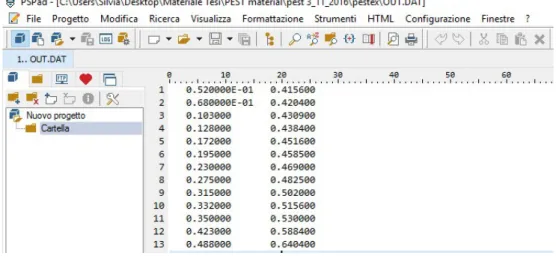
Figure 16. out.dat output file. ... 55

Figure 17. Template file in.tpl. ... 56

Figure 18. in.pmt file. ... 56

Figure 19. File in.par in which the values of SCALEs are all equal to 1.0, OFFSETs equal to 0.0 and PRECIS and DPOINT are ‘single point.’ ... 57

Figure 20. Instruction file out.ins. ... 57

Figure 21. File out.obf. ... 58

Figure 22. File measure.obf. ... 59

Figure 23. Control file twofit.pst. ... 59

Figure 24. Modified section of twofit.pst file. ... 60

Figure 25. Comparison of experiment results calculated in different ways. ... 61

Figure 26. Modified control file twofit.pst. In the red circle there is the PARTRANS modified of parameter s1. ... 62

Figure 27. twofit.par changed after the modification of the control file. ... 62

Figure 28. Changes applied to the model code twoline.for. To notice the comments in red. ... 63

Figure 29. Modified twoline.for with two more parameters h and k. Highlighted in red the changed steps. ... 65

Figure 30. New results from file out.dat. ... 66

Figure 31. File twofit.par. New values of parameters estimated with PEST. ... 66

Figure 32. Modified code for twoline.exe in order to have a more complex output file. ... 67

Figure 33. New format of output file out.dat after having modified the model executable twoline.exe. ... 67

(10)

2

Figure 34. New version of file out.ins. ... 68

Figure 35. Conceptual model of the WW-01 well-reservoir system: it is possible to see the well WW-01 and the formation ... 69

Figure 36. WW-01 wellbore-reservoir model 2D vertical section ... 70

Figure 37.Initial pressure and temperature conditions assumed for the wellbore-reservoir model ... 70

Figure 38. Comparison between measured and simulated flowing pressures.. ... 71

Figure 39. Input file for T2Well-PEST application. ... 73

Figure 40. PEST template file called WW-01_0.9.tpl. ... 73

Figure 41. File .pmt, where all the parameters names are listed, generated by using the utility tool TEMPCHEK. ... 74

Figure 42. File .par, where all the parameters names and values are listed, generated by using the utility tool TEMPCHEK. ... 74

Figure 43. FStatus_2.ins instruction file. ... 75

Figure 44. File FStatus_2.obf generated from INSCHEK tool. ... 76

Figure 45. File experimental_data.obf. ... 76

Figure 46. Control file generated with PESTGEN, called tough2_WW01.pst. ... 78

Figure 47. Final output file FStatus_2. ... 79

Figure 48. tough2_WW01.par containing the estimated parameters set. ... 80

Figure 49. Graph showing the matching between the experimental data, the manually simulated dataset and the values obtained from PEST calibration.. ... 80

List of Tables

Table 1. Experimental data table... 52

Table 2.Reservoir formation horizontal permeability as obtained by manual calibration of the model. ... 71

(11)

(12)

(13)

5

1.INTRODUCTION

The calibration of a model (i.e. the research of the best values to be assigned to its parameters) is a complex task that in general requires to spend a lot of work. This is particularly true in the field of the reservoir engineering where the possibilities to have reliable measured data is rare because of both the high measurement costs and the low reproducibility of measures. Moreover, a reservoir model is characterized by a huge number of different parameters and often the data refers to different measurement techniques using different measurement units. Well calibrated models will produce robust and reliable simulations. Therefore, the possibility to have available a reliable tool to automatize the process of calibration surely improve the task of the reservoir engineer.

In particular, we are interested to work with wellbore-reservoir coupled high enthalpy geothermal models. Therefore, we have used PEST (Model-Independent Parameter Estimation, a program software for the parameter estimation and analysis of the uncertainties of environmental models and in general of complex numerical models) coupled with T2Well-EWASG (a wellbore-reservoir simulator, which uses the equation of state EWASG (Equation-of-State for Water, Salt and Gas), dedicated to multiphase-multicomponent geothermal high enthalpy reservoir) to enhance the calibration task. It is noteworthy to highlight that, PEST-T2Well-EWASG could be also used to improve the interpretation of well-tests performed on geothermal reservoirs.

Before facing with the practical issues of coupling the PEST and T2Well and using their tools and keywords, it is useful to briefly clarify some fundamental concepts, necessary for understanding the concept of simulation in general. In particular, the meanings of the terms system, process, model, numerical model, simulation, geothermal reservoirs, etc., will be defined.

1.1 System and model definitions and classification

The system is defined as an interacting set of parts which form an individual “body” that allows the process (a transmission of energy, mass or information) to occur. In our case the system will be a geothermal reservoir. Generally, system has two categories of properties that characterize its

(14)

6

behavior: parameters, properties of the system invariant respect to the time, and variables that change through the time because of the interaction between the system and the external world. An example of a parameter of an aquifer could be the compressibility of water, while a variable could be the distribution of the water pressures inside the aquifer.

A system can be schematized as an entity, in which a process occurs, and that has relations with the external environment through an input and an output. The output (or response) of the system will depend on the actions that the external world exerts on the system (said inputs or solicitations or perturbations) and on what happens within the system itself, that is its internal state. The system output U(t) can be mathematically represented as a function f that depends on another function that describes the internal state S(t), on a function that describes the external solicitations I(t) and on a set the set of model parameters p1, p2, …, :

( ) = ( ), ( ), 1, 2, … (1.1)

In the case of geothermal aquifers, one input can be the start of production of vapor from the production well with a defined flow rate; the response may be the pressure variation of the fluids, while the internal state can be described by the distribution of the saturations, and the parameter can be the porosity, the permeability etc., …, .

In real cases, it is very difficult or often impossible to properly know all the characteristics of a system, or sometime it is impossible to work directly on the system itself, thus the system is studied using a simplified version called model. The model includes exclusively the more important aspects of the system that affect the analyzed problem. The model could be of different types: physical model, that can be a scale model in which the elements of the system are represented in scale; analog model, in which the system properties are represented through different physical quantities or symbolic models where the system is represented by symbols that can be handled. An example of symbolic model is the mathematical model in which equations and functions are used to represent the system and that can be divided in two categories: analytical and numerical models. Analytical models will provide, if any, an exact solution for the system, while numerical models develop an approximate solution that is reasonably close to the expected results. Given that very often it is impossible to find a solution of the analytical model, the numerical one is the only tool to represent adequately the behavior of the system.

(15)

7

- According to the exchanges of matter and energy: a system is said open (from the thermodynamic point of view) when it exchanges both matter and energy with the external environment.

If the exchange of energy and matter is not allowed, it is said isolated, and if it is not allowed only the exchange of matter, is said closed. The geothermal reservoirs, in general, are open systems.

- Depending on the time variation of parameters: A system in which the same stress, repeated at different times, produces the same output, is said invariant. It is, however, inevitable that the parameters vary with time, as an effect of the aging process; the systems in which the parameters vary in time are called variants. It is possible to assume, however, that, despite a system is variant, the parameters that characterize it, are constants on sufficiently small time intervals. For example, the porosity, on long time intervals can vary as a result of the compaction of the rock, however it can be assumed that remains constant in a sufficiently short period of time, for example over a period of a few months.

Thus it is the rate of change of the parameters compared with the speed of evolution of the system which determines the invariance of the system.

- Depending on the time variation of variables: Depending on whether the variables that describe the system are constant or not in time, the systems are defined: static or dynamic. For a system to be defined as dynamic is sufficient that only one of the variables mutates over time.

- According to the values assumed by the variables: The type of variables of the system, continuos or discrete, subdivides the system in continuous or discrete respectively. In the first case the variables have a biunivocal correspondence with the real number set. In the second case the variables have a biunivocal correspondence with the set of natural numbers, or with a finite subset of them.

-Depending on the properties of relations: If the relationships between dependent variables and independent variables allow the determination of the value of a dependent variable in a unique way, the system is said deterministic. Otherwise, if the relationships among the dependent variables and the independent ones require the adoption of statistical relations, it is called stochastic or probabilistic system.

Lastly, observing the output of a system as a result of the input solicitations, the concept of steady-state and transient can be defined. The steady state is the state in which the system has

(16)

8

finished its evolution and produces a constant output or tending asymptotically to a value, said steady output. The transient state is instead the state in which the system is in evolution between two states of regime and the output tends to stabilize towards the steady output of the second state.

(17)

9

1.2 Calibration of the model

After the selection of the appropriate model to represent the system under investigation, there is the interpretation phase, in which the system output data obtained from the preliminary tests are interpreted using the model. This phase is used in important activities like the model calibration and analysis of sensitivity and error propagation [Bortolotti, 2013].

More specifically, the calibration operation involves the estimation of the values of constants and parameters regarding the model structure. In order to do this, it is necessary to compare the observed variables with that of the output produced by the run of the model and to try to reduce the discrepancies between the two set of variables. The observed variables are obtained from experiments, thus in general, the estimation step looks for the values of parameters that have the higher probability of being accurate taking into account the error tolerance: trial-and-error method (general scheme shown in Figure 1).

This procedure could be implemented by hand, with severe limitation, or by means of specific software. Another way to calibrate the model is to use parameters and constants values derived from a different model estimation in another location similar to the currently studied area. This last method should be utilized by experienced users only.

The sensitivity analysis is a procedure to identify the intensity of the model output especially as a consequence of the variation of its parameters. In other words, the research of the parameters that more influence the behavior of the model (and therefore of the system). This analysis is important to figure out which laboratory measurements or in situ must be improved. Parameters that do not affect significantly the model do not require to be measured or estimated with high precision. While the error propagation analysis allows to study the impact of the uncertainty of parameter values on the predictions made by models, through the analysis of the propagation of errors or Monte Carlo simulation, which provides correlations between parameters.

(18)

10

Figure 1. General scheme of a model calibration [Taylor et al, 2012].

When a satisfactory estimation of the parameters of the considered model have been obtained, the model should perform adequately the scope for which it was created, therefore its behavior must be checked. This process of the verification of a calibrated model is called validation [Institute of Transportation Engineers, 1992].

The conventional simulation technique determines the output of a calibrated model for a given set of initial conditions and time history to obtain information regarding the system behavior in its future evolution.

The inverse simulation is the reverse of the previous type of simulation, in fact in this case, the time history of a selected system output variable is laid down and the algorithm of the inverse simulation bring the investigator to calculate the time history of the corresponding input variable. Inverse modeling, parameter estimation, history matching and model calibration are terms essentially describing the same technique. They aim to assess the best model and its parameters for predicting the behavior of a dynamic system [Finsterle, 2007].

(19)

11

Figure 2. Summary scheme that relates all the notions linked to models explained in the paragraph 1.1 and 1.2 [Baveye et al., 2007].

1.3 High enthalpy geothermal reservoirs

1.3.1 Geothermal energy

Energy from the Earth's interior that flows through its surface is on average very low. Anyway, it is sufficiently abundant to make it locally worth exploiting. In fact, only in the top 3 km of the Earth's crust stores an estimated 4.3 × 107 EJ of thermal energy due to the rocks temperature and their thermal capacity. The principal geothermal potential is from heat flowing through the crust. Where geothermally heated, water rises to the surface in hot springs. Sometimes in this case, it has been used directly for heating, recreational and horticultural purposes since Roman times, while this type of energy was used indirectly for the first time when geothermally generated electricity was produced in 1904 at Larderello, Italy.

The interior of the Earth becomes hotter with increasing depth for two reasons:

- heat is generated by the decay of some natural radioactive isotopes (238 and uranium-235, thorium-232 and potassium-40);

- heat flows from the hot interior by means of convection and conduction.

The geothermal heat flows through the Earth determines a geothermal gradient (the rate at which temperature increases with depth). The geothermal gradient variation beneath the continental

(20)

12

surface is shown in Figure 3, where it is possible to notice that temperature increases much more with depth in the lithosphere than in the deep mantle.

Figure 3. The geothermal gradient, the temperature increases more rapidly with depth in the lithosphere than it does in the deep mantle

(http://www.open.edu/openlearn/science-maths-technology/science/environmental-science/energy-resources-geothermal-energy/content-section-1).

Even if they are not melted rocks, rocks forming the deep mantle are hot enough to behave in a ductile way. Parts of the hotter mantle rise slowly because they are slightly less dense than cooler mantle, this is a physical transport of heat towards the surface. This process is called convection and is an efficient means of heat transport.

Except at plate boundaries and hotspots convection, this method does not transfer heat in the lithosphere. Instead heat is transferred by conduction, which is a far less efficient process than convection, so the lithosphere acts as an insulating blanket (trapping the heat rising from below). Harvesting geothermal energy depends on the relationship between heat flow through the lithosphere and the local geothermal gradient.

The most favorable areas for geothermal exploitation seems to be those in volcanically active regions, at destructive and constructive plate margins. It is less obvious that is also worth exploiting some areas that are remote from volcanically active regions.

(21)

13

The local potential of geothermal energy is described by the enthalpy H of the area (total energy content of the geothermal system that lies below it). The enthalpy of a system cannot be measured directly: only a change or difference in energy has physical meaning. Enthalpy is a thermodynamic potential, so in order to measure the enthalpy of a system, one must refer to a defined reference point. Therefore, what is measured is the change in enthalpy, ΔH. At constant pressure, the ΔH equals the energy transferred from the environment through heating (the heat flow through the crust, measurable at the surface).

The equation of enthalpy is:

= + (1.2)

Where, U is the internal energy of the system, p is the pressure of the system, V is the volume of the system.

The Figure 4 shows that large areas of the Earth's surface have basically the same heat flow. However, the temperature at depth in the crust depends on how conductive the different rocks are, and this in turn depends on their physical properties. This subsurface temperature is crucial in evaluating whether or not an area constitutes a geothermal resource.

Figure 4. World map showing variation in surface heat flow in mW m−2_{in relation to continental and oceanic crust, and major}

plate boundaries. The colors relate to the scale in mW m−2_{. There are areas in continents where heat flow does rise to very high}

values, but they are too small to show on this map (http://www.open.edu/openlearn/science-maths-technology/science/environmental-science/energy-resources-geothermal-energy/content-section-1).

In a general classification, there are three types of area with geothermal potential; those with high, medium and low enthalpy.

 High-enthalpy areas are those where subterranean water and steam are at temperatures greater than 180 °C;

(22)

14

 Medium-enthalpy areas those where temperatures range between the boiling temperature of water (100 °C) and 180 °C;

 Low-enthalpy areas where temperatures are lower than 100 °C.

Using geothermal energy effectively speeds up heat flow and locally increases the heat lost by the Earth. But geothermal heat is continually supplied, so hot water and steam are depleted faster rather than the energy resource itself. However, if hot fluids removed are replaced by cold water pumped to recharge the geothermal field, the cold water heats up again. Carefully managed recharge enables the enthalpy of an area to be exploited continuously.

Geothermal fields usually need three characteristics to be exploited successfully: 1. An energy source to heat the fluids;

2. An aquifer, either natural or artificially created, to act as a reservoir for fluids that can transport heat energy to the surface;

3. A cap rock with low permeability to seal in these geothermal fluids (in a similar way to the trapping of petroleum). [Sheldon, 2005; Smith, 2005].

High- to medium-enthalpy geothermal resources are conventionally divided into water- or vapor-dominated fields. Vapor-vapor-dominated systems where the steam is at high temperature and dry tend to be the most economically viable geothermal resources, because the pV term in the enthalpy equation is high. Vapor-dominated fields also suffer less from problems of corrosion from the mineral-laden waters that are typical of deep aquifers. When such hot water passes through pipelines, not only it is highly corrosive, but solids dissolved in it precipitate in the pipes as temperature decreases, and could clog them, [Sheldon, 2005].

1.3.2 Locating high-enthalpy geothermal fields

The research of potentially useful geothermal fields is focused initially on locating rocks that have been chemically altered by natural geothermal fluids, looking for obvious surface features of geothermal activity (geysers and hot springs). Then, the fluid flow measurement through the field permits the estimation of the probable economic potential of the reservoir.

After that a promising resource has been located, the exploration wells are drilled. However, given the high pressures and temperatures typical of a geothermal resource, special precautions must be taken. For example, once the drill stem penetrates a superheated water saturated zone,

(23)

15

the liquid will flash to steam as the pressure drops and this is very dangerous. The well head itself is capped with valve gear to regulate the flow of fluids, and the whole assembly is then conveyed to an electricity generating plant [Sheldon, 2005].

1.3.3 The pros and cons, and future of geothermal energy

If correctly exploited, the geothermal energy is renewable but the geothermal fluids emit gases such as CO2, H2S, SO2, H2, CH4 and N2 when used for electricity generation. However,

geothermal power plants are usually sited in areas of natural geothermal activity, where such emissions occur anyway. Other potential pollutants are various ions dissolved in the geothermal fluids, but these are almost always returned to the reservoir when the spent fluids are re-injected. Regarding safety, accidents are usually rare. Protracted geothermal exploitation can induce ground subsidence, although this is minimized by re-injecting spent fluids. Small intensity earthquakes can sometimes result from large-scale exploitation. Anyway, most high-enthalpy geothermal areas are naturally predisposed to seismicity.

The main disadvantage of geothermal power generation is that suitable high-enthalpy areas are geographically very restricted, many being in areas of low population density (or under the sea). On the contrary, the low-enthalpy potential of normal heat flow is universal and potentially useful for heating and even air conditioning, given the necessary investment.

In the short term, even twenty- to forty-fold growth in geothermal capacity will not result in it being a significant contributor to global energy needs by 2020. Geothermal power plants are generally much smaller than fossil-fuel and nuclear generators; tens of MW, rather than a few GW for the biggest “conventional” plants. To replace a single GW fossil fuel power station requires from 20 to 33 geothermal plants. The seeming benefit of local and 'environmentally friendly' geothermal power generation, because of economic factors related to their construction, delays its adoption at national to international scales [Sheldon, 2005].

1.3.4 Generalities on the simulation of geothermal reservoirs

The simulation of geothermal reservoirs is closely related to the one of the hydrocarbon reservoirs, which began in the ‘50s. The simulation by means of numerical models of the subsurface has rapidly evolved in recent years, thanks to the use of ever more advanced digital techniques and the availability of computers with computing capabilities continuously growing. It

(24)

16

has also increased the demand for a quantitative estimation of movement and heat transfer processes in the subsurface.

A good methodology in the creation of models allows one to increase the reliability of the simulation results, in fact, the determination of the objectives of the operation at the start of the modeling and the possible results, allows a more effective use of simulation [Bedient, 1999]. Moreover, although the simulation of a geothermal reservoir is often required by the competent authorities to grant permissions to exploitation, it is often necessary to integrate a numerical simulation with other tools in order to get a better analysis of the site on which it must operate. A typical scheme of the project of numerical models is the following:

1. Definition of the simulation objective: for example, in the case of geothermal reservoirs can be the prediction of the values of pressure and temperature as a result of putting into production of new wells;

2. Development of a conceptual/geological model of the system (geometry, zoning, spatial distribution of petrophysical properties, initial saturation in fluids and initial pressures, etc...); 3. Identification of the thermodynamic parameters of the fluids in the reservoir and their spatial variations; definition of the curves of relative permeability and capillary pressure;

4. Choice of the equations that govern the processes and of a simulation software. Both must be verified: the equations must describe the physical, thermodynamic, chemical and biological processes that has been established to simulate, while the code, that implements these equations, must be verified by comparing the numerical results with the analytical solution to a known problem;

5. Definition of the grid ("mesh"): it defines the discretization in blocks of the system's spatial domain. It must be appropriate to reproduce the volume occupied by the field, of the boundary conditions and of particular conformations of the subsurface such as faults or fractures;

6. Model initialization: to each block are assigned the values of petrophysical parameters of the rocks, and initial thermodynamic and fluid dynamic values of fluids present in the reservoir. The combination of phase 5 to 6 constitute the so-called pre-processing, namely the creation of the data needed to process the numerical model, which will be stored in a simulator input file;

7. Model calibration or history matching; 8. Sensitivity analysis;

9. Predicting the behavior of the model in terms of future programs of the reservoir cultivation, or use in forecast mode. The analysis of results is also called post-processing;

(25)

17

10. Corrections and changes to the model according to the results of the simulations.

1.3.5 Problems related to the use of numerical models for the simulation of geothermal reservoirs

A lack of the use of numerical models in the simulation of geothermal systems is that they require large amounts of input data, which are often too expensive and difficult to obtain, so that often either simplifying assumptions are made or values obtained from the literature are adopted, that cannot be closely representative of the real properties of the reservoir.

The values of parameters measured in situ are intended as the average or total values of the area involved (for example by means of pumping tests, transmissivity and storage coefficient of the aquifer are obtained), which cannot reflect a particular local situation of the field. On the other hand, values obtained in the laboratory (such as permeability or porosity) on cores, are only representative of the area in which the sampling of the material has been made, which can have very different characteristics from the surrounding areas.

The attempt to model a system, of which there are few data available, is the same a useful operation as it allows one to identify areas where a greater number of information are needed, increasing in this way the understanding of the reservoir [Bedient, 1999].

The need to have results in reduced times requires the use of very powerful computers and therefore expensive; despite the adoption of the most powerful computers available on the market, the detail of the grids cannot massively increase, as well as the precision of calculation, all this to the detriment of the accuracy of the final results of the simulation.

The use of numerical models in the oil field has highlighted the need and the priority to focus the efforts on finding the most likely geological model of the reservoir and its internal structure and share the tasks, within the simulation team, in function of the individual skills [Chierici, 2004]. The calibration of the model, obtained by means of the solution of the so-called inverse problem, allows to obtain a validated model; such model is not necessarily unique: they may exist in fact several models (different distributions of parameters) that reproduce the past history of the reservoir, but only one can be used as the real one.

Although the model validation phase is mandatory, it does not guarantee that the validated model can forecast the future behavior of the reservoir [Chierici, 2004]. It is also no possible to prove that the results of a simulation are correct [Bedient, 1999].

(26)

18

The sensitivity analysis is performed by varying, within a reasonable range, the values of one parameter at a time and comparing the results of the series of simulations. This allows one to determine the influence of the uncertainty of parameters on the final response of the simulation. This procedure allows one to determine the most likely values of parameters; the studies of sensitivity are the most realistic way of use of numerical models for the prediction of reservoirs behavior [Chierici, 2004].

1.4 T2Well in brief

T2Well is a coupled wellbore-reservoir numerical simulator for non-isothermal, multiphase, multicomponent flows. This software was created as an extension of the numerical reservoir simulator TOUGH2 to calculate the flow simultaneously and efficiently in both the wellbore and the reservoir, by introducing a special wellbore subdomain into the numerical grid. For the wellbore subdomain grid-blocks, the 1D momentum equation of the mixture (which may be two-phase) is solved as described by the Drift-Flux Model (DFM, explained later in paragraph 1.4.1), [Pan and Oldenburg, 2012]. The equations are numerically solved with the Integrated Finite Difference Method. The IFDM is a numerical method for approximating the solution to differential equation using finite difference equations to approximate derivatives [Bortolotti, 2015]. This method is characterized by a geometrical grid constraint: the connecting segment between the centers (or nodes) of two close blocks must be perpendicular to the interface between the two blocks. Structured grids always satisfy this constraint, as the blocks are either cubes or parallelepipeds or radial sections, whereas in case of unstructured grids, the Voronoi tessellation must be used [Berry et al., 2014]. In Figure 5 are reported the different possible types of grids as reported by Berry at al., 2014.

(27)

19

Figure 5. Different possible types of grids [Berry et al., 2014].

T2Well coupled with an adequate Equation of State (EOS), that manages the fluids thermodynamic of the system, can be used to simulate the commonly exploited high enthalpy geothermal systems. To deal with high enthalpy geothermal reservoir characterized by water, salts and one non-condensable gas, T2Well was coupled with the EOS EWASG (Equation-of-State for Water, Salt and Gas, see paragraph 1.4.2).

In the following subparagraphs, there will be both a generic explanation of the equations used by T2Well and of the structure of its input and output files.

1.4.1 Mass and energy balance and Drift Flux Model

The equations for the mass and energy conservation used by T2Well have the same structure as in TOUGH2:

= ∙ + (1.3)

Where Vn is the volume of an arbitrary element of the system and Γn is the closed surface that

bounds the element volume. On the left side of the equation 1.3, which is the accumulation term, Mk represents the quantity of mass or energy per volume, where the label κ can assume 1,…,NK values when it represents the mass components (that could be water, air, solutes or H2) and NK+1

(28)

20

values in energy balance case. On the right side, the vector n is the normal to the surface element dΓn and Fk represents the mass or heat flux term, the second integral with qk denotes sinks and

sources terms [Pruess et al., 1999].

The main differences from the equations used for the porous media by TOUGH2 are in the energy flux, energy accumulation and in the computation of phase velocity in the subdomains representing the wellbore. T2Well uses the DFM briefly described in the following, to calculate the velocity of both liquid and gaseous phases.

The DFM was first developed by Zuber and Findlay (1965) and it represents a valid alternative for the two-phase flow study in a pipe. More in detail it is used for the phase velocities determination without solving the equation of the momentum for each phase. This model is based on some empirical constitutive relationships, in which all the variables must be considered either as area-averaged or constant over a cross-section. The main relationship is the following equation:

= + (1.4)

which establishes that the gas velocityv_G, can be related to the volumetric flux of the mixture j, and the drift velocity of the gas,v_d, via the parameter C₀, named profile parameter, which takes in account for the effect of local gas saturation and velocity profiles over the pipe cross-section [Pan et al, 2011].

In the case of subdomain grid-blocks representing the wellbore, the 1D momentum equation of the mixture, which may be two-phase, (liquid and gas for example) is solved according to the DFM. Here the mixture velocity is calculated by solving numerically the momentum equation, whereas the velocities of individual phases are calculated from the mixture velocity. More in detail, the pressure gradient, gravity component, and time derivative of momentum are treated fully implicitly, while the spatial gradient of momentum is treated explicitly. The friction term is calculated with a mixed implicit-explicit scheme [Pan and Oldenburg, 2012].

(29)

21 1.4.2 EWASG module

Considering that geothermal fluids usually consist of complex mixtures of water, salts and gases, and their thermodynamic and transport properties affect reservoir conditions and performance, as mentioned before, the EWASG module was developed for the TOUGH2 multi-purpose numerical reservoir simulator to handle three-component fluid mixtures of water, sodium chloride and a slightly soluble non-condensable gas (NCG) [Battistelli et al., 1993; 1997].

Since 1999 EWASG has been available to the public within the TOUGH2 V.2.0 package [Pruess et al., 1999]. Sodium chloride (NaCl), is used to simulate the effects of dissolved salts, whereas the effects of one NCG were included following a general formulation in which the NCG can be chosen by the user among a set of implemented NCGs (in the TOUGH2 V.2.0 package, the NCGs available are CO2, CH4, H2, N2, air and O2 added more recently). So, the multi-phase

system is assumed to be composed of three mass components: water, sodium chloride, and one NCG, (carbon dioxide for conventional geothermal applications).

All the relevant thermophysical properties are evaluated by means of a subroutine structure, so that the correlations currently used can be easily modified as soon as more reliable experimental data and correlations become available. It is assumed that the three phases (gaseous, liquid, and solid) are in local chemical and thermal equilibrium, and that no chemical reactions take place other than interphase mass transfer [Calore and Battistelli, 2003].

As mentioned before, the thermo-physical property correlations used in EWASG, are accurate for different conditions of geothermal reservoirs, as an example, the fluid pressure can be up to 80 MPa, temperatures can vary in a range between 100 and 350°C, CO2 partial pressure can arrive

up to 10 MPa and salt mass fraction up to halite saturation.

1.4.3 Input and output files

Being T2Well based on the TOUGH2, their input files are very similar, however there are small differences that will be explained in this paragraph. Let’s first describe shortly the TOUGH2 input file.

To characterize a flow system, TOUGH2 requires many data including hydrogeological parameters and constitutive relations of the permeable medium, as relative and absolute permeability, porosity, capillary pressure; fluids thermophysical properties, initial and boundary

(30)

22

conditions of the flow system, sink and sources. It requires also the specification of space-discretized geometry, program options, computational parameters and time-stepping information. All these data must be provided to TOUGH2 in one or more ASCII data files within a fixed format with up to 80 characters per record. All the information is organized in blocks and reported in the standard metric (SI) unit system.

Here below, the main keywords used in a typical TOUGH2 input file are described briefly (it is possible to see the complete list of the input file and keywords in the TOUGH2 v.2.0 manual [Pruess et al.,1999]):

- ROCKS describes the rock types providing also the hydrogeological parameters as porosity, permeability, heat conductivity and specific heat…;

- ELEME and CONNE provide the mesh geometric information like nodes coordinates, areas of interface; in ELEME the rock type for each grid block is also specified;

- MULTI specifies the fluid components number and grid block balance equations; - SELEC provides the thermophysical properties data;

- PARAM defines all the parameters for the computation such as program options, time steps and simulated time;

- GENER is used to define sources and sinks;

- INCOM and INDOM permit to define the initial conditions.

An arbitrary record, with arbitrary data, that do not start with a TOUGH2 keyword will be ignored, permitting to directly insert comments in the input file. TOUGH2 will collect all these comments and write them as records in the output file. Figure 6 shows a piece of a TOUGH input file with all keywords explained before.

(31)

23

Figure 6. TOUGH2 input file example.

All the specific parameters of T2Well are stored under the keyword ROCKS, and they must be introduced only for the wellbore ROCKS types, as follows:

ROCKS----1----*----2----*----3----*----4----*----5----*----6----*----7----*----8 wellb NAD 2600.0 1.0 1.0E-13 1.0E-13 1.0E-13 -2.1 1000.0 0.0 0.0 2.1 0.0 0.0 1 0.2 0.1 0.9 0.7 1 0.0 0.0 1.0 NTEMP RWB UHT ZF(1) TF(1) ZF(2) TF(2) … ZF(NTEMP) TF(NTEMP)

The first four record are the traditional ones, referring to the properties of the rocks (density, porosity, permeability, thermal conductibility, in the first record specific heat, in the second record pore compressibility and expansion, heat conductivity in desaturated conditions, tortuosity factor and Klinkenberg parameter, in the third record relative permeability function parameters and in the fourth record capillary pressure function). The new records follow and are read only if NAD (first record, second field) is larger than 3. Thus, after the record of the capillary pressure, it is possible to introduce the following parameters:

NTEMP: number of couples (cell depth; formation temperature) with which the code will determine the corresponding formation temperature at the wellbore cell depth. If NTEMP is equal

(32)

24

to 0, the temperature of the formation is taken equal to the initial temperature of wellbore, otherwise the code will read the couples depth-temperature in the following NTEMP records; RWB (m): the completion radius;

UHT: the over-all heat transfer coefficient;

It is possible, by proper rock type introduction, to take into account different parts for the same wellbore, characterized by different parameters, such as the wellbore and the completion radius, the over-all heat transfer coefficient. Furthermore, characterizing the wellbore, for example, with two different rocks type, it is possible to apply an analytical computation of heat exchange only for a wellbore portion, for which, for modelling purpose, the surrounded formation must not be explicitly modelled. In fact, the analytical computation of heat exchange between wellbore and reservoir is possible only if the model is composed by the wellbore (no grid blocks of surrounding formation) and it is activated if the thermal conductivity (CWET) of the wellbore rock type is negative. With the keyword NAD it is possible to select the type of wellbore reservoir heat exchange analytical relation [Vasini, 2016].

Regarding the main output file, here will be reported only a brief summary, for more details see TOUGH2/ECO2N manual [Pruess, 2005].

The formats of the output file are basically the same as that of TOUGH2/ECO2N except that a profile of velocities (of the mixture, gas, and liquid phase) in the wellbore is added next the regular profile output (at user specified output steps). In addition, some informational outputs regarding wellbore cells, connections, and their geometry features are also included in the front of the main output file. In addition to the TOUGH2 output, T2Well gives two additional information: FStatus and FFlow that are briefly described below together with the other files with fixed name. These description are taken from the ”TWell/ECO2N Version 1.0: Multiphase and Non-Isothermal Model for Coupled Wellbore-Reservoir Flow of Carbon Dioxide and Variable Salinity Water” [Pan et al., 2011].

-FStatus: five status variables of each wellbore cell at every time step and depth: time, distance to wellhead, gas saturation, mass fraction of CO2 in liquid, pressure, temperature, gas density; - Fflow: five variables of each wellbore connection at every time step and depth: time, distance to wellhead, liquid phase mass flow rate, gas phase mass flow rate, liquid phase velocity, gas phase velocity, mixture velocity;

(33)

25

- FOFT: optional (transient output of state variables for user-specified cells in main input file. First two variables are the index and the simulation time, respectively. They are followed by the cell index and five variables at the cell in turn of each cell listed in FOFT section of the main input file. The five variables are pressure, gas saturation, mass fraction of CO2 in liquid phase, mass fraction of salt in liquid phase, and the temperature, respectively.);

- COFT: optional (transient output of flow rate and velocity for user-specified connections in main input file. Data structure here are very similar to FOFT, except for that here the five variables are gas phase mass flow rate, liquid phase mass flow rate, gas phase velocity, liquid phase velocity, and total CO2 mass flow rate, respectively, for each connection listed in COFT section in the main input file.);

(34)

(35)

27

2. PEST TOOLS

The acronym PEST stands for Parameter Estimation and was originally created for model calibration in which the parameter values are calculated with inverse modelling by matching the output of the model to the values of measurements of the system state. PEST is different from the others parameter estimation software because it works in a model-independent way, in fact PEST interacts with the model through its own input and output files.

In a few words, PEST runs many times a executable program representing the model (program-model in short) every time with different values of some parameters of a program-(program-model in order to minimize the difference from the output of the models and a set of experimental data. Therefore PEST must be able to interact with the input and output files used by the program-model.

PEST run a program-model through a call to the operating system (OS), process named system call, that has the same effect as typing the model name in the command line window. For this reason the program-model must be accessible to a user through the command line. In practice, the folder in which the model is stored the program-model should be inserted in the PATH environment variable of the OS so that the OS knows where to find it.

If a model prompts the user for keyboard input, then the process of calibration apparently seems not to be automatable, but this situation can be easily accommodated. In fact the keyboard responses to the model's prompts can be placed into a text file and the model will import the answers from this file (see below for details). In this way, PEST can run the model without needing any user involvement [Doherty, 2016].

Therefore using PEST it is possible to automatize the calibration of a generic model as long as its executable is accessible and usable via a terminal way (command line approach).

More in detail, to execute a calibration run, PEST requires three types of input file:

 template files, in which all the parameters are defined for each input file of the studied model;

 instruction files, one for each model output file on which model-generated observations exist;

(36)

28

 control file, supplies PEST with all template and instruction files names, corresponding model input and output files names, the problem size, control variables, initial parameter values, measurement values and weights, etc. … .

Once having built these files, it is possible to use the utility programs TEMPCHEK, INSCHEK and PESTCHEK to check both their correctness and consistency.

2.1 Model Input files and PEST template files

PEST provides a set of parameter values which it wants the model to use for a particular run. These data are generally taken from the model input file.

Some models read their data from the terminal prompt, the user must supply these data in response to model prompts, but this can also be done through a file. It is possible to redirect the responses to the model, that the user has been previously written in a file, through the terminal redirection < symbol (redirection is a form communication between process of a many OSs). Therefore if the model in question is run using “model” command, and the responses are typed in advance to a file named for example file.inp, then PEST can run the model without supplying the terminal input using the command:

model < file.inp

If the file.inp contains some parameters that PEST must optimize, it is possible to create a template for it as if it were any other model input file.

The template file instructs PEST to read the input files of the simulator and is necessary only for those input files which contain parameters that require an estimation. Generally, an input file of a model can be of any length, however PEST requires that it is less than 2000 characters in width. The same applies to the template files and it is suggested that template files have to be provided with “.tpl” extension in order to distinguish them from other file types. Basically a template file is simply a model input file replica except that the space occupied by each parameter in the latter file is replaced by a sequence of characters which identify the space that the parameter occupies. The first line of a template file must contain the letters ptf (PEST template file) followed by a parameter delimiter explained later. It is possible to see the examples of a PEST input file and its relative PEST template file taken from PEST Manual in Figure 7 and Figure 8 respectively.

(37)

29

Figure 7. Example of PEST input file.

Figure 8. Example of PEST template file.

Both input and template file are necessary to create the PEST control file explained later.

2.1.1 The parameter delimiter

The parameter delimiter is the equivalent of the field format of Fortran, indicates the boundaries in which PEST will read the input file of the model. The parameter delimiter is a single character that follows the keyword “ptf” after a blank space in the PEST template file (# in Figure 8). In a template file, a parameter space is identified as the set of characters limited by and including two parameter delimiters. When PEST writes a model input file based on a template file, it replaces all characters between and including these parameter delimiters by a number representing the

(38)

30

current value of the parameter that owns the space; that parameter is identified by name within the parameter space, between the parameter delimiters.

The characters [a-z], [A-Z] and [0-9] are invalid to identify the parameter delimiter. The defined parameter delimiter must appear nowhere within the template file except in its parameter delimiter capacity, in fact wherever PEST finds that character in the template file it assumes that it is delimiting a parameter space.

2.1.2 Parameter names

All parameters are referenced by a name, these references are necessary in template files (in which the parameters locations on model input files are identified), in control file (where parameter initial values and lower and upper bounds are provided), and in input files which contains parameters that PEST has to process. Parameter names cannot exceed twelve characters in length and are case-insensitive, moreover any characters is allowed except for the space character and the parameter delimiter chosen previously.

Given that each parameter space is defined by two parameter delimiters, the parameter name to which the space belongs must be written between the two delimiters.

2.1.3 Setting the Parameter Space Width

Numbers can be represented with greater precision in wider spaces than in narrower spaces, anyway PEST can adjust to limited precision in parameters representation on model input files, as long as sufficient precision is employed in order to distinguish a parameter value from the value of that same parameter incremented for derivatives calculation. It could be useful to provide the values of the parameters with as much precision as the model is able to read them with, in this way they can be provided to the model with the same precision with which they have been calculated by PEST.

Generally the numbers are read by the models either from the terminal or from an input file in two different ways: namely from specified fields, or as a sequence of numbers (of any length); the latter method is often referred to as free field input or as list-directed input. Notice how no

(39)

31

whitespace or comma is needed between numbers which are read using a field specifier. Very often, a model input file is used as starting point for the construction of a template file. In such input file, numbers are read using free field input and are often be written without trailing zeros, for this reason during the construction of the template file it has to be recognized where there are free field input numbers and consequently expand the parameter space (to the right) in respect to the original number, leaving whitespace or a comma between successive spaces, or between a parameter space and a neighboring character or number.

In a similar way, numbers read through field-specifying format statements may not occupy the full field width in a model input file, in this case, during the template file compilation, it should be necessary, again, to expand the parameter space beyond the extent of the number (here to the left of the number only) until the space coincides with the field defined in the format specifier.

2.1.4 Preparing a Template File

The preparation of a template file is very simple procedure, in many models it is done just by using a text editor, coping the input file and replacing the parameter numerical values with their respective parameter space and name identifiers. As mentioned before, one time that the template file has been created, its correctness can be checked using the TEMPCHECK utility program. This program can also write a model input file which will be based on the template file and a user-supplied list of parameter values. Then, if the model is run with the provided TEMPCHEK-prepared input file, the model will not have difficulties in reading the PEST TEMPCHEK-prepared input files.

2.2 Instruction files

For each output file of the model that contains observations, an instruction file has to be provided to PEST in order to instruct the program to follow its directions which PEST must follow to read that file. This instruction file has to have the extension “.ins”. The first line of a PEST instruction file must begin with the three letters “pif” (PEST instruction file).

Remember that if an output file is more than 2000 characters in width, PEST will not read it. Pay attention that given that the precision in the representation of model-generated observations is

(40)

32

essential, unlike the precision of parameter values, it is possible to vary with any control variables the precision with which a model’s output data are written in order to have the maximum available precision. Also this file together with input and template files is used to generate the control file.

2.2.1 How PEST Reads a Model Output File

PEST must be taught how to read a model output file (that must be a text file) and identify the numbers it must extract from that file. A list of instructions on how to find data on an output file must be provided to PEST, instead of using a template for an output file.

Essentially, PEST acts in the same way as a person does. Both run eyes down the file looking for something that is known, a marker properly selected to link to it the observations. In case of simple models, more in detail single-purpose models where small development time has been invested in highly descriptive output files, no markers are necessary, the default initial marker will be the top of the file. It is possible to have either primary or secondary markers. PEST employs primary marker to scan the model output file line by line, looking for a reference point for subsequent observation identification or further scanning, while it uses a secondary marker as a reference point given that a single line is examined from left to right.

2.2.2 The Marker Delimiter

The role of the marker delimiter in an instruction file is not unlike that of the parameter delimiter in a template file, it must be placed just After the acronym “pif” and a single space and before the first character of a text string comprising a marker and immediately after the last character of the marker string and it has to define the extent of a marker. The portion of text between a pair of marker delimiters is not interpreted by PEST as a set of instructions. The choice of the marker delimiter is limited, in fact it cannot be one of the following characters: A - Z, a - z, 0 - 9, !, [, ], (, ), :,&, the space or tab characters and it should not occur within the text of any markers as this will cause confusion to PEST.

(41)

33 2.2.3 Observation Names

Each observation has to be provided with a unique name that must be twenty characters or less in length. These characters can be any ASCII characters except for [, ], (, ), or the chosen marker delimiter character. These same observation names must also be cited in the PEST control file where measurement values and weights are provided. These rules do not apply to the dummy observation name, “dum”; it can occur many time in an instruction file if necessary and signifies to PEST that although the observation is to be located as if it were a normal observation, the number corresponding to the dummy observation on the model output file is not actually matched with any laboratory or field measurement. Thus, a “dum” observation must not appear in a PEST control file where measurement values and observation weights are provided. The dummy observation is simply a device for model output file navigation.

2.2.4 The Instruction file keywords

When an instruction file is created, it has to be provided with a precise and clear syntax which must be followed exactly. The instruction items on a single line must be separated by at least one space. Instructions in a single line of a model output file are written on a single line of the PEST instruction file. So the new instruction line start implies that PEST must read at least another one new model line of the output file, the number of lines that it has to read depends on the first instruction on the new instruction line. If the first instruction on the new line is the character “&”, that like the others instruction items has to be separated from its following instruction item by at least one space, it means that the new instruction line is simply a continuation of the old one. PEST reads the model output file in top-to-bottom (forward) direction and it is important to remember that an instruction cannot direct PEST to read a previous line on the output file. Here following are reported the main keywords for the instruction file:

(42)

34

Primary Marker

The primary marker has already been discussed briefly. On encountering a primary marker in an instruction file PEST reads the model output file, line by line, looking for the string between the marker delimiter characters. When it finds the string it places its “cursor” at the last character of the string. If any other instruction as the primary marker on the same instruction line directs PEST to further processing this line, that processing must pertain to parts of the model output file line following the string identified as the primary marker. If in a primary (or secondary) marker there are blank characters, exactly the same number is expected to match the string on the output file of the model. It should be noted that despite the utility of markers, the search for a primary marker is a very time-consuming process as each line of the model output must be individually read and scanned for the marker.

Line Advance

The syntax for the line advance item is “ln” where n is the number of lines to advance. The line advance item must be the first item of an instruction line; it and the primary marker are the only two instruction items which can occupy this initial spot. Unlike the case of the primary markers, in implementing a line advance, PEST does not have to examine the model output file lines while it advances. It simply moves forward n lines, placing its processing cursor just before the beginning of this new line, this point will become the new reference point for more processing of the model output file. Generally a line advance command is followed by other instructions. If a line advance item precedes the first instruction line of a PEST instruction file, the reference point for line advance is taken as a “dummy” line just above the first line of the model output file. Secondary Marker

A secondary marker is a marker which does not occupy the first position of a PEST instruction line. Hence it instructs PEST to move its cursor along the current model output file line until it finds the secondary marker string, and to place its cursor on the last character of that string ready for subsequent processing of that line. If a particular secondary marker is preceded only by other markers, and the text string corresponding to that secondary marker is not found on a model output file line on which the previous markers’ strings have been located, PEST will assume that it has not yet found the correct model output line and resume its search for a line which holds the text from all the markers. When it will find a line with both primary and secondary markers, it

(43)

35

will commence the next instruction line execution. If any instruction items different from the markers precede an unmatched secondary marker, PEST will consider that mismatch an error condition and will stop the execution displaying an appropriate error message. Remember that also the secondary markers may be used sequentially.

Whitespace

The whitespace instruction is similar to the secondary marker in that it allows the user to navigate through a model output file line prior to reading a non-fixed observation. It directs PEST to move its cursor forwards from its current position until it encounters the next blank character. PEST then moves the cursor forward again until it finds a nonblank character, finally placing the cursor on the blank character preceding this nonblank character ready for the next instruction. The whitespace instruction is a simple “w”, separated from its neighboring instructions by at least one blank space.

Tab

The tab instruction places the PEST cursor at a user-specified character position (i.e. column number) on the model output file line which PEST is currently processing. The instruction syntax is “tn” where n is the column number. The column number is obtained by counting character positions (including blank characters) from the left side of any line, starting at 1. Like the whitespace instruction, the tab instruction can be useful in navigating through a model output file line prior to locating and reading a non-fixed observation.

Fixed Observations

First of all, it is necessary to specify that an observation reference can never be the first item on an instruction line. As for the others instructions, if there are different observation on a particular line of the model output file, these must be read from left to right and cannot be read backward along the line. To identify observations it is possible to say to PEST that a particular observation can be found between and also including columns n1 and n2 on the output file line of the model

where the cursor is resting at that moment. This is the best way to read an observation value because PEST simply has to read a number from the space identified without doing any research. This type of observations is called “fixed observations”. The instruction for PEST for reading a