Chapter 6 Calibration of deteriorating model with laboratory tests

(1)

Chapter 6 Calibration of deteriorating model with laboratory tests

6.1 Abstract

In this chapter the pre-defined Ibarra-Medina-Krawinkler deteriorating model with bilinear response has been used to model several beam-to-column connection. In order to calibrate the deteriorating parameters that control the behavior of the model, both monotonic and cyclic analysis have been performed and the results have been compared with the ones obtained in real tests performed by the Department of Steel Construction of RWTH Aachen University within a research project for modern plastic design of steel structures, named PLASTOTOUGH [19].

6.2 Material

The material used in these tests has been steel S355J2, which is one of the materials of highest economical interest for profiles of structures subjected to both seismic and static loads. The main characteristics of the material have been summarized in the following tables, both for pates and profiles.

≤3 ≤16

(2)

6.3 Geometry of the test

For the rotational tests welded beam-column joints have been investigated where the column consists of a HEM 300 profile and the beams either of profiles HEA 300 or IPE 500. In Figures 6.1 and 6.2 the principal geometry of the beam-column test specimen is provided.

Fig. 6.1: Geometry of rotation test – specimen with profiles HEA 300 [19]

Fig. 6.2: Geometry of rotation test – specimen with profiles IPE 500 [19]

The column and the stiffeners welded within are selected in this way in order to avoid plastic deformation and instabilities in the column itself. Both monotonic and low cycle fatigue tests have been performed.

The tests have been conducted with two different welding details in order to differentiate the performance of a detail sophisticated for seismic loading from a non sophisticated detail. For the non sophisticated joint the flange and web of the beam have been welded by fillet welds to the column. For the sophisticated connection the flange is connected to the column by a butt weld. The flanges are chamfered with an angle of 35° and then welded to the flange of the column. After welding of the butt weld the root of the weld is sealed by an 8 mm fillet weld.

(3)

a) b)

Fig. 6.3: Weld details – a) non sophisticated (fillet weld); b) sophisticated (butt weld) [19]

6.4 Testing procedures for cyclic tests

The tests have been performed in control of deformation and stepwise under variable an constant amplitude loading conditions. According to ECCS procedure [18] at first a monotonic test has been performed in order to evaluate the deformation values at yield load. They have resulted:

 for profiles HEA 300  for profiles IPE 500

Beside the ECCS history which has been performed for both profiles, other loading procedure have been applied to the models.

6.4.1 Procedure for HEA 300 specimens

6.4.1.1 ECCS procedure 6.4.1.2 95% fractile procedure 6.4.1.3 Kobe procedure

(4)

6.4.1.4 Constant amplitude procedure

6.4.2 Procedure for IPE 500 specimens

6.4.2.1 ECCS procedure

6.4.2.2 Mean value procedure

6.4.2.3 Constant amplitude procedure

6.4.3 Summary of the tests

6.4.3.1 Nomenclature

, , , , , . Other parameters are:

6.4.3.2 Table of monotonic tests

(5)

6.4.3.2 Table of cyclic tests

Table 6.4.II: Cyclic tests

6.5 OpenSees Model used

6.5.1 OpenSees materials used

To ensure a non linear behavior of the column only non-linear behavior material have been considered. Specifically:

 Uniaxial Material Steel01 [ref. par. 3.5]

 Modified Ibarra-Medina-Krawinkler deterioration model with bilinear hysteretic

response [ref. par. 3.9]

6.5.2 OpenSees sections used

The sections used to model the non linear behavior of the connection have been:  Fiber section [ref. par. 3.6]

 Zero-length section [ref. par. 3.6]

6.5.3 OpenSees elements used

The element used to model the non linear behavior of the column have been:  Elastic Element [ref. par. 3.7]

(6)

6.5.4 OpenSees Model

The model of the Beam-to-column connection has been realized following the “concentrated plasticity” concept, as already described in Par. 5.6.1. Beams and columns are modeled using pre-defined Elastic Beam-Column Element connected to Zero-Length

Elements, which serve as rotational springs to represent the structure’s nonlinear

behavior. The springs follow a bilinear hysteretic response based on the Modified

Ibarra-Medina-Krawinkler deterioration model with bilinear hysteretic response [ref. Par. 3.9].

The input parameters for the rotational behavior of the plastic hinges have determined using empirical relationship developed by Lignos and Krawinkler in 2010 [10]. An idealized scheme of the model is presented in Fig. 6.4 and Fig 6.5, in which spring’s and rigid links size have been greatly exaggerated for clarity.

Fig. 6.4: Beam to column connection – Nodes

Fig. 6.5: Beam to column connection – Elements

Where:

(7)

Since a frame member is modeled as an elastic element connected in series with rotational springs at the end, the stiffness of this component must be modified so that the equivalent stiffness of this assembly is equivalent to the stiffness of the actual frame member. Based on the approach described in Appendix B of Ibarra and Krawinkler [8], the rotational springs are made “n=10” times stiffer than the rotational stiffness of the elastic element in order to avoid numerical problems and allow all damping to be assigned to the elastic element. To ensure the equivalent stiffness of the assembly is equal to the stiffness of the actual frame member, the stiffness of the elastic element must be times greater than the stiffness of the actual frame member. In this example, this is accomplished by making the elastic element’s moment of inertia times greater than the actual frame member’s moment of inertia.

In order to make the nonlinear behavior of the assembly match that of the actual frame member, the strain hardening coefficient (the ratio of post-yield stiffness to elastic stiffness) of the plastic hinge must be modified. If the strain hardening coefficient of the actual frame member is denoted and the strain hardening coefficient of the spring

(or plastic hinge region) is denoted then:

The theoretical parameters used for the definition of the backbone curve of the zero-length rotational springs have been calculated using the predefined relations provided by Krawinkler and Lignos [9-10] (see Par. 2.5). A MathCAD sheet has been used and the results are shown below.

(8)

(9)

The following tables summarize all the parameters requested by OpenSees for the definition of the Moment-Rotation backbone curve for the plastic hinges. This give also information about all the theoretical value, obtained by using the above defined relations, as well as the practical values used in all the simulated tests. One can see that for some test the input value of a parameter is much different from the theoretical one. The reason is attributable to the fact that the relations used to define the theoretical value of the parameters derive from cumulative distribution, so that they have mainly a statistical significance.

Cross section: HEA 300

(10)

(11)

6.5.4.2 Cross section IPE 500

For the analytic evaluation of the parameters required, in the case of cross section IPE 500, both the general equations and the specific ones for beam depth have been considered, in order to understand the difference and the trend for deep sections.

(12)

The following tables summarize all the parameters requested by OpenSees for the definition of the Moment-Rotation backbone curve for the plastic hinges. This give also information about all the theoretical value, obtained by using the above defined relations, as well as the practical values used in all the simulated tests. One can see that for some test the input value of a parameter is much different from the theoretical one. The reason is attributable to the fact that the relations used to define the theoretical value of the parameters derive from cumulative distribution, so that they have mainly a statistical significance.

(13)

Cross section: IPE 500

(14)

Table 6.5.II: Deteriorating model – Requested parameters for IPE 500

6.6 Results for monotonic test

In Figures 6.6 – 6.9 the Load vs Displacement curves are shown for both profiles. One can see the good correspondence with the real test results.

The main differences between the two cross section are:

 The HEA 300 section is characterized by soft hardening after yield and smooth transition in post-capping branch of the relation. The IPE 500 section, instead, has higher hardening but is characterized by a sheet post-capping branch.

 The HEA 300 section is characterized by a pre-capping rotation which is around 1,5 times the one of IPE 500. The post-capping rotation of the HEA is almost 2 times the one of IPE.

(15)

6.6.1 HEA 300 specimens

Fig. 6.6: Load-displacement curves for profile HEA 300 [19]

Fig. 6.7: OpenSees model – load-displacement curves for profile HEA 300

0 100 200 300 400 500 600 700 0 25 50 75 100 125 150 175 200 225 250 Force [kN] Displacements [mm[ test BT_HEA_355_ns-1 test BT_HEA_355_s-1

(16)

6.6.1 IPE 500 specimens

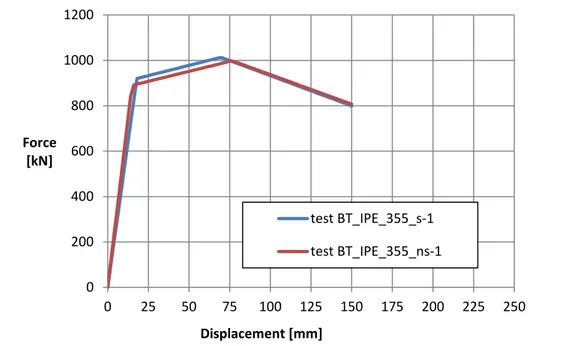
Fig. 6.8: Load-displacement curves for profile IPE 500 [19]

Fig. 6.9: OpenSees model – load-displacement curves for profile IPE 500

One can also observe a difference between the two weld details:

 The butt welded specimen is characterized by a lower initial stiffness, a lower yield force but a smoother post-capping branch, differently to the fillet welded specimen.

 The difference in stiffness between the two details is amplified in the unloading branch. 0 200 400 600 800 1000 1200 0 25 50 75 100 125 150 175 200 225 250 Force [kN] Displacement [mm] test BT_IPE_355_s-1 test BT_IPE_355_ns-1

(17)

6.7 Results for cyclic tests

All the results are given in terms of Moment-Rotation diagrams. The rotation, expressed in Radians, is the average between the rotation of node 2 and node 4. Because of the geometry of the tests, the value of Moment of node 32, expressed in kNm, corresponds of the value of the vertical force applied by the loading machine, expressed in kN. In facts:

Being the effective length of the beam, taking account of the length of the rigid link.

A red line ( ) has been inserted in all the following displacement pattern in order to remark the displacement that corresponds to the first yield of the section. The results have been:

 for cross-section  for cross-section

6.7.1 HEA 300 specimens

6.7.1.1 RT-HEA-355-ns2: ECCS PROCEDURE

The general ECCS procedure is specified in Par. 6.4.1. In RT-HEA-355_ns-2 test the procedure consists in the application of the following displacement pattern:

Fig 6.10: RT-HEA-355_ns-2 test – Displacement pattern

-200 -150 -100 -50 0 50 100 150 200 0 5000 10000 15000 20000 25000 30000 Displacement Node 3 [mm] Time steps

(18)

6.7.1.2 RT-HEA-355-s2: ECCS PROCEDURE

The general ECCS procedure is specified in Par. 6.4.1. In RT-HEA-355_s-2 test the procedure consists in the application of the following displacement pattern:

Fig 6.11: RT-HEA-355_s-2 test – Displacement pattern

6.7.1.3 RT-HEA-355-ns3: 95% FRACTILE PROCEDURE

The general 95% fractile procedure is specified in Par. 6.4.1. In RT-HEA-355_ns-3 test

the procedure consists in the application of the following displacement pattern:

-150 -100 -50 0 50 100 150 0 5000 10000 15000 20000 25000 30000 35000 Displacement Node 3 [mm] Time steps -60 -40 -20 0 20 40 60 0 20000 40000 60000 80000 Displacement Node 3 [mm] Time steps

(19)

6.7.1.4 RT-HEA-355-s3: 95% FRACTILE PROCEDURE

The general 95% fractile procedure is specified in Par. 6.4.1. In RT-HEA-355_s-3 test the procedure consists in the application of the following displacement pattern:

6.7.1.5 RT-HEA-355-ns4: KOBE PROCEDURE

The general Kobe procedure is specified in Par. 6.4.1. In RT-HEA-355_ns-4 test the procedure consists in the application of the following displacement pattern:

-60 -40 -20 0 20 40 60 0 10000 20000 30000 40000 50000 Displacement Node 3 [mm] Time steps -80 -60 -40 -20 0 20 40 60 80 0 20000 40000 60000 80000 100000 120000 Displacement Node 3 [mm] Time steps

(20)

6.7.1.6 RT-HEA-355-s4: KOBE PROCEDURE

The general Kobe procedure is specified in Par. 6.4.1. In RT-HEA-355_s-4 test the procedure consists in the application of the following displacement pattern:

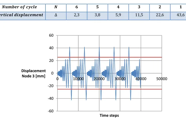
6.7.1.7 RT-HEA-355-ns5: CONSTANT AMPLITUDE PROCEDURE

The general Constant Amplitude procedure is specified in Par. 6.4.1. In RT-HEA-355_ns-5

test the procedure consists in the application of the following displacement pattern:

-80 -60 -40 -20 0 20 40 60 80 0 20000 40000 60000 Displacement Node 3 [mm] Time steps -80 -60 -40 -20 0 20 40 60 80 0 20000 40000 60000 80000 Displacement Node 3 [mm] Time Steps

(21)

6.7.1.8 RT-HEA-355-s5: CONSTANT AMPLITUDE PROCEDURE

The general Constant Amplitude procedure is specified in Par. 6.4.1. In RT-HEA-355_s-5

test the procedure consists in the application of the following displacement pattern:

-80 -60 -40 -20 0 20 40 60 80 0 10000 20000 30000 40000 50000 60000 Displacement Node 3 [mm] Time Steps

(22)

6.7.2 IPE 500 specimens

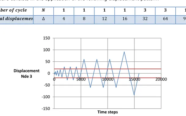
6.7.2.1 RT-IPE-355-ns2: ECCS PROCEDURE

The general ECCS procedure is specified in Par. 6.4.2. In RT-IPE-355_ns-2 test the procedure consists in the application of the following displacement pattern:

Fig. 6.18: RT-IPE-355_ns-2 test – Displacement pattern

6.7.2.2 RT-IPE-355-s2: ECCS PROCEDURE

The general ECCS procedure is specified in Par. 6.4.2. In RT-IPE-355_s-2 test the procedure consists in the application of the following displacement pattern:

Fig. 6.19: RT-IPE-355_s-2 test – Displacement pattern

-150 -100 -50 0 50 100 150 0 5000 10000 15000 20000 Displacement Nde 3 Time steps -80 -60 -40 -20 0 20 40 60 80 0 5000 10000 15000 20000 25000 30000 35000 Displacement Node 3 [mm] Time steps

(23)

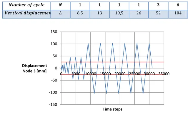
6.7.2.3 RT-IPE-355-ns3: MEAN VALUE PROCEDURE

6.7.2.4 RT-IPE-355-s3: MEAN VALUE PROCEDURE

-50 -40 -30 -20 -10 0 10 20 30 40 50 0 10000 20000 30000 40000 50000 Displacement Node 3 [mm] Time steps -50 -40 -30 -20 -10 0 10 20 30 40 50 0 10000 20000 30000 40000 50000 Displacement Node 3 [mm] Time steps

(24)

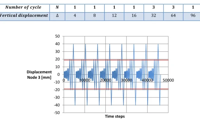
6.7.2.5 RT-IPE-355-s4: CONSTANT AMPLITUDE PROCEDURE

6.7.2.6 RT-IPE-355-s4: CONSTANT AMPLITUDE PROCEDURE

-60 -40 -20 0 20 40 60 0 10000 20000 30000 40000 50000 Displacement Node 3 [mm] Time Steps -60 -40 -20 0 20 40 60 0 10000 20000 30000 40000 50000 D isp lac e m e n t N o d e 3 [m m ] Time Steps

(25)

In the following images the Moment-Rotation diagrams for all the simulated cyclic displacement-controlled tests are shown.

As already explained in the chapter, in the X-axis of the curves is the moment developed by Node 32, thus the moment of the left deteriorating spring.

Instead, in the Y-axis, the average between the rotation of node 2 and node 4 is represented.

Fig. 6.24: Quantities used in Moment-Rotation diagrams

One can see the good correspondence with the results obtained by real tests, under very different displacement pattern. One can conclude that Ibarra-Medina-Krawinkler

deterioration model with bilinear hysteretic response is a powerful instrument to model

(26)

Fig. 6.25: RT-HEA-355_ns-2 test [ECCS PROCEDURE] – Moment-Rotation diagram -800 -600 -400 -200 0 200 400 600 800 -0,100 -0,050 0,000 0,050 0,100

M

Fig. 6.38: RT-IPE-355_s-4 test [CONSTANT AMPLITUDE PROCEDURE] – Moment-Rotation diagram -1200,0 -1000,0 -800,0 -600,0 -400,0 -200,0 0,0 200,0 400,0 600,0 800,0 1000,0 1200,0 -0,040 -0,020 0,000 0,020 0,040

M [kNm

]

j

[rad]

RT-IPE-355_s-4

(40)

6.8 Influence of the hardening stiffness in the model

Analyzing the results of some tests it’s evident that the OpenSees model, despite it fixes well the real tests in almost all the cycles, it’s characterized by a bigger total dissipated energy. Therefore a new set of data has been used in order to limit this difference. The following table describe the two set of used data.

The goodness of the new set of data has been tested by performing one of the previus cyclic displacement controlled tests, specifically the RT-HEA-355_ns-5 test [CONSTANT AMPLITUDE PROCEDURE]. The result is shown in the following diagram, where the new results are represented in green. -800 -600 -400 -200 0 200 400 600 800 -0,050 -0,040 -0,030 -0,020 -0,010 0,000 0,010 0,020 0,030 0,040 0,050

M

[

kNm]

j

[rad]

RT-HEA-355_ns-5 PLASTOTOUGH OPENSEES

(41)

One can observe the new curve doesn’t fix the real test curve (blue curve) in the first cycle, but the two curves are really similar in the last cycles. In adduction one can note that the total energy dissipated in the real test seems to be more similar with the new set of data (green) than the one with the old one (red).

6.8 Conclusions

The main conclusions than derive from this chapter are exposed in the follow:

 Different cyclic displacement-controlled procedure have been applied on the OpenSees Model of the beam to column connections. Despite this, the visual analysis of the result, compared to the ones obtained within real tests, show a remarkable correspondence, both within the elastic and the inelastic branches of the behavior. The correct input of the deterioration parameters in the model is the key to obtain this. Therefore it’s of primary importance an accurate evaluation of them.

 The empirical relations provided to determine the deterioration parameters are characterized by a general validity. Therefore it’s important, for an accurate definition, to compare them with the value obtained from the wide database of tests provided by the authors or, if available, from laboratory cyclic tests.

 Comparing the theoretical values of the deteriorating parameters and the used ones, that allow the model results to fix the real tests, results evident that both the Cyclic deterioration parameter for strength deterioration and for post-capping strength

deterioration need to be approximately doubled in order to obtain correct results even

in the last displacement excursions. On the opposite, regarding the deterioration parameter for unloading stiffness deterioration, this value need to be minor than the theoretical one, in order to catch the correct slope of the unloading branches of the last cycles.

 Observing the results on can note that the HEA 300 section is characterized by soft hardening after yield and smooth transition in post-capping branch of the relation. The IPE 500 section, instead, has higher hardening but is characterized by a sheet post-capping branch. The HEA 300 section is characterized by a pre-post-capping rotation which is around 1,5 times the one of IPE 500. The post-capping rotation of the HEA is almost 2 times the one of IPE.

 Even the two analyzed weld details show a slightly different behavior. In fact the butt welded specimen seems to be characterized by a lower initial stiffness, a lower yield force but a smoother post-capping branch, differently to the fillet welded specimen. The difference in stiffness between the two details is amplified in the unloading branch.