Cros-Organism Annotation Prediction through Deep Learning Algorithms

(1)

ALMA MATER STUDIORUM - UNIVERSITA' DI BOLOGNA CAMPUS DI CESENA

SCUOLA DI SCIENZE

CORSO DI LAUREA IN INGEGNERIA E SCIENZE INFORMATICHE

CROSS-ORGANISM ANNOTATION PREDICTION THROUGH DEEP LEARNING ALGORITHMS

Relazione finale in

Programmazione di applicazioni Data Intensive

Relatore Presentata da

Prof. Gianluca Moro Marcello Feroce

Co-Relatore

Dott. Ing. Roberto Pasolini

Sessione 5 Ottobre 2017 Anno Accademico 2016/2017

(2)

Cross Organism annotation

prediction through deep learning

algorithms

Marcello Feroce

October 5, 2017

Abstract

Studying how genes or proteins influence humans and other species’ lives is paramount. To study that, it’s necessary to know which functional properties are specific for each gene or protein. The association between one gene or protein and a functional property is called annotation. An annotation can be 0 or 1. 1 means that gene or protein contributes to the acti-vation of a certain functional property. Functional properties are referred by terms, which are strings that belong to ontolo-gies. This work aim is to predict novel gene annotations for little know species such as Bos Taurus. To predict such anno-tations, a model, built using deep learning, is used. This model is trained using well know species as Mus Musculus or Homo Sapiens. Every predicted annotation has its own likelihood, that tells about how much the prediction is close to a 0 or a 1. Final accuracy can be evaluated fixing a certain value of like-lihood, so that all the considered annotations have a likelihood greater or equal than the fixed one. The obtained accuracy is quite high but not enough to be used in a professional way, although it offers a nice cue for future research.

(3)

1 Introduction

Knowledge of how structural or functional biological prop-erty of a living being can differ from being to being has a primary importance. It helps understanding physiological and patholog-ical biologpatholog-ical processes, as well as developing new drugs and therapies.

Aim of this work is to predict novel structural or functional bio-logical properties of little know organisms, which are little stud-ied by biologists, for several reasons. Functional biological prop-erties, which can be referred by terms, short unique strings ba-sically, tell us a lot about how a living being can differ from an other. One example can be the ability of a cell to reproduce it self. These functional biological properties are depending on genes and proteins(which depend on genes). So, being able to predict functional biological properties, could simplify a lot the work of biologists, and understanding how a living being behave, depending on its genes would be much faster than it is nowadays. Of course a very high accuracy is necessary, and it has to be ob-tained in a relatively short time.

Next sections will show in a more accurate way all the steps taken to get the results. Starting with an introduction to the do-main, annotation prediction in literature will follow. An explana-tion of Machine Learning and Deep Learning is necessary then of course before starting explaining in a more specific way how the prediction works. Indeed the algorithm used and the choices are explained, followed by the technologies used. Finally Exper-iments and results are exposed.

1.1 Domain of the work

To have a clearer idea on how the project works it’s necessary to have clarify some basic concepts.

(5)

included in all the possible biomolecular entities of its species. Biomolecular entities are mainly genes and protein products. Species have also a set of possible structural or functional biological properties which can be working or not. A property can be part of a subset of properties, or be itself a subset of properties, thus containing different properties which all respect its function. Making an instance to understand better, the property "having a volume enclosed by the nuclear inner membrane" is part of the property "having any constituent part of the nucleus, a membrane-bounded organelle of eukaryotic cells in which chromosomes are housed and replicated" but also of the property"having an organelle lumen that is part of an intracellular organelle".

Biomolecular entities are identified by an abbreviation. Struc-tural or functional biological properties refer to terms, which are part of ontologies. Ontologies contain terms and define their structure through a Directed Acyclic Graph (DAG). The Gene Ontology (GO) is the most considerable. The DAG shows the hierarchies of the terms with IS_A and PART_OF relationships. The schema of the DAG would look as a tree. A controlled biomolecular annotations(often referred just as annotations) is an association between a biomolecular entity and a term in an ontology.

(6)

Figure 1: Representation of a DAG. Got from this work[1]

An annotation matrix A(g, t) is a binary matrix whose i-th row A(g i , t) is the annotation profile of the gene g i to the terms t ∈ T ; thus, a binary gene-term annotation matrix A(g, t) represents a set of known annotations of some genes g to some controlled terms t ∈ T. This means that there could be several annotation matrix for each species, having different subsets of biomolec-ular entites and terms, and different values of the annotations, depending on the year and on the research.

(7)

Table 1: example of GO term

id: GO:0000016 name: lactase activity namespace: molecular_function

def: "Catalysis of the reaction: lactose + H2O = D-glucose + D-galactose." synonym: "lactase-phlorizin hydrolase activity" BROAD [EC:3.2.1.108]

synonym: "lactose galactohydrolase activity" EXACT [EC:3.2.1.108] xref: EC:3.2.1.108

xref: MetaCyc:LACTASE-RXN xref: Reactome:20536

is_a: GO:0004553 ! hydrolase activity, hydrolyzing O-glycosyl compounds

Each annotation in the annotation matrix is represented by 1 either a 0. If it’s 1, it means that the biomolecular entity in that row activates(by itself or with other biomolecular entities) that term in that column.

There are some annotation matrices, called Inferred from Elec-tronic Annotation (IEA), whose annotations are computed. These ones are as not reliable as the normal ones, but they can be useful anyway.

Some biomolecular entities can be included in more annotation matrices of different species, since more species can have part of biomolecular entities which are in common. The same speech could be done for terms: Different species can have same prop-erties.

(8)

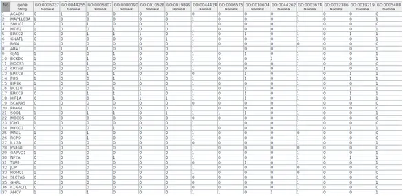
Figure 2: Example of annotation matrix

In general, annotation matrices have thousands of genes and terms, and are sparse matrices, i.e. matrices in which most of the elements are zero.

1.2 Aim of the work

As introduced at the beginning of the chapter, prediction is the mainly thing this project has to do. Having clarified some concepts in the previous section allows to explain better the aim of the work.

Having some genes of a little know species, thus with a very few known annotations, there should be a program which returns the annotations associated with those genes for a certain set of terms. Trying to predict novel gene annotations, there are several meth-ods that can do that or at least give a contribute. In this work a neural network, which is the model used in deep learning, a sub-type of machine learning, has been used. Several other methods can be used, but working with neural network could be a good idea, after the good results obtained in this work[1] with machine learning. In this method there is a preliminary work that has to be

(9)

done previously of building the model. This preliminary work is in a certain way similar to the one exposed in the method used in this work[1], that is the one this work is inspired by. This prelim-inary work’s aim is fundamentally to get the right and best anno-tations that will be used to train and use the model. In the field of bioinformatics, annotation prediction is very useful, but it’s only one of the possible aims that bioinformatics has. Some of them are completely different, but many others are very related to an-notation prediction, and can be useful in anan-notation prediction. Other times instead, annotation prediction is attempted, but with completely different approaches.

2 Annotation prediction in literature

Predicting novel gene annotations has a primary importance, as told before. It comes hard in general to predict them in a short way with even a great accuracy. As we will see flex-ibility and speed go to the opposite way than valuable prediction. Many computational approaches have been proposed to find out novel annotations of biomolecular entities through the processing of different kinds of experimental data as biomolecular sequences, gene expressions, protein interactions and phylogenetic profiles, worked out using different techniques such as sequence homology, network based or data and text mining based methods [38][39]. Multiple types of data have been approached in several tries, even from different species through comparative genomic approaches. These attempts pursued to improve results(e.g., [41][40]]). These approaches and methods are usually pretty complex and very costly, and didn’t show great results.

Many different methods or approaches have been tried in order to predict new biomolecular annotations through

(10)

compu-tational techniques:

A latent semantic approach to build a prediction algorithm based on the Singular Value Decomposition (SVD) method with gene-to-term annotation matrices[6][7]. The algorithm basically counts co-occurrences between pairs of annotation terms. As in the work in [8] this algorithm was improved. They computed gene functional similarity on the GO annotations of the genes and used it to include gene clustering. Then, they extended it, being able to automatically choose the best SVD truncation level. The SVD has also been used with annotation weighting schemes[9][10][11], built on term and gene frequencies. Al-though very adaptable on the organism and the term vocabulary, these methods brought limited accuracy.

As in this work [42], a prototypal multi-organism Genomic and Proteomic Data Warehouse, called GPDW, was built, to predict gene annotations basing on on information and data integration, using SVD, and SIM(Semantic improvement), but they didn’t get excellent results.

In this work [43] researchers worked on Protein Annotation Prediction using Metric Labeling and Semi-metric Embedding. They got quite good results, although their method didn’t show robustness.

Sophisticated latent semantic analysis techniques, mainly related to Latent Semantic Indexing (LSI)[12] have been proposed to predict biomolecular annotations on the basis of available annotations leveraging on available annotations. These were formerly used for Natural Language Processing. These techniques include the probabilistic Latent Semantic Analysis(pLSA)[13], which uses the latent model of a set of annotation terms to improve reliability of annotation prediction

(11)

results. This technique was used in [14] and was improved with weighting schemes[15]. This brought an improvement comparing to the SVD method in this work [16].

Latent Dirichlet Allocation (LDA) algorithm has been at the basis of topic modeling in this work[17]. LDA was also used in two works[18][19] to separate gene expression microarray data in clusters. LDA algorithm associated with the Gibbs sampling[21][22][23] was improved to predict gene annotations in this work[20]. Despite these complex techniques are far better than the ones based on linear algebra, these are not good when the data size increase due to slowness.

Also biological network analysis is frequently used to pre-dict gene functions:

As in the work in[24], GeneMANIA was built. GeneMa-nia is a server whose purpose is gene function prediction. GeneMania takes the inputs(query gene sets) as networks whose associated weight is based on the strength of the connectivity between the genes in the query set, compared with their connec-tivity to non-query genes.

As in the work in [25] reserachers instead leveraged on a kernel-based learning method whose approach is based on a labeled graph kernel which can predict functions of single genes basing on the function distributions which can be evaluated from their associated gene interaction networks.

Tecniques from Hidden Markov Model(HMM) were also used to get a model of the evolution of genes[26], or to predict gene function basing on sequential gene expression data[27]

(12)

and Bayesian networks to predict annotations by learning patterns from available annotations.

In the work in[29], researchers suggested a k-nearest neighbour (k-NN) classifier to associate a gene with new annotations common among its functionally nearest neighbour genes. In this method gene functional distance is computed according to the semantic similarity of the GO terms that annotate the genes.

Gene function prediction techniques use also a lot of Sup-port Vector Machine (SVM) classifiers:

SVM classifiers were used in this work[30] to predict an-notations for many eukaryotic protein sequences. Another work[31] instead leveraged them to predict potential functions for previously unannotated Drosophila melanogaster genes, analysing a huge dataset from gene expression microarray experiments.

New supervised methods have come recently, even for an-notation prediction. Two examples are the works [32]. and [33].. The first one considered the prediction of gene functions as a multi-label top-down classification problem. This method is based on hierarchical relationships in the GO structure that soften the quantitative difference in quantity, between negative and positive samples used for training. Cheng et al.’s work showed low accuracy.

The second one suggested that relations between genes generate autocorrelation in gene annotations and breach the assumption that annotations are independently and identically distributed. Stojanova et al. got better a slightly better accuracy.

Another used solution to predict novel gene annotations is to use multiple data types or sources, even from different

(13)

species. Several experiments have been done. An example is this work [34], where researchers built a general Bayesian framework to integrate heterogeneous types of high-throughput biological data. The Bayesian framework was applied for the prediction of Saccharomyces cerevisiae gene functions.

a SVM classifier for each gene annotation to a GO term was trained in this work[35]. using gene expression levels from microarray experiments. Further consistency among predicted annotation term was enforced by means of a Bayesian network mapped on the GO structure.

Differently, text mining techniques were used in this work[36] and in this other work[37] to extract from the literature gene associated keywords which are then mapped to GO concepts. These approaches got better results with compared to similar methods applied on a single data type but, a preparatory data integration step is needed, and this adds complexity, decrease flexibility and slows the prediction process. Thus, formerly suggested methods for biomolecular(gene or protein) annotation prediction either are general and flexible, but show low accuracy, or get better results by either working with a complex integrative analytical framework or adopting a more complex model. The reason for the low accuracy is mainly given from the simple model used. On the other hand, leveraging a complex integrative analytical framework is often hard and takes a long time to be set up. Using a more complex model instead heavily slows the prediction process, in particular when the testing data size increases a lot.

3 Methods

A model is needed to predict novel gene annotations. This model has to be built with annotation matrices of very well known(and so studied) species. The model would show all its power working with annotation matrices of little know species

(14)

as input.

3.1 Machine learning

Not always a program runs a clear and procedural algorithm written by someone. In the cases it doesn’t, sometimes it’s pos-sible to say that the programs uses machine learning algorithms. Machine learning consists in a self-made learning of a knowl-edge model from a huge amount of example data, called training set. Machine learning build the aforesaid model generalising pat-terns observed in the training set.

Unlike the usual way to program, in machine learning, programs are taught how to process data, from examples.

Lots of approaches can be used with machine learning. Some of them are Decision tree learning, Association rule learning, Deep learning.

Each of these approaches can address a wide variety of tasks as: • Classification

• Regression: Find a pattern between variables

• Clustering: Unlike classification, the groups are not known beforehand

• Density estimation: Finds the distribution of inputs in some space

• Dimensionality reduction: Maps the input into a lower-dimensional space

Tasks can also be classified in another way. Usually they are split in three large categories, depending on the "feedback" received during the learning:

• Supervised learning • Unsupervised learning

(15)

• Reinforcement learning

3.2 Deep learning

Deep learning is a subtype of machine learning whose model is a neural network

3.2.1 Neural Networks

Neural networks are the models used by deep learning. Neu-ral networks, whose name actually should be "Artificial neuNeu-ral networks", have this particular name because they are inspired by the biological neural networks that constitute animal brains. Neural networks can implement many tasks among the ones of machine learning. Neural networks are very used to implement regression and Classification.

Each neural network consists in one input layer, one output layer, and an indefinite number of hidden layers, which could be even 0. However usually the number of layers goes from two to four. Each layer includes nodes. In the input layer nodes consist in the inputs given to the model.

Each layer can have a different number of nodes. Between two layers there are other two components:

• Weights • Biases

The number of weights between two layers corresponds to the number of nodes in the first layer(the one closer to the input layer) multiplied by the number of the nodes in the second layer. Indeed, for each couple of nodes there is a weight.

The number of biases between two layers corresponds to the number of nodes in the second layer(the one closer to the out-put layer).

The value of each node of the next layer is given by this easy procedure:

(16)

• Multiply each node in input with its weight that refers to that node in output

• Sum the previously obtained values

• Sum an offset value, called bias, to the value previously obtained

• Apply to the obtained value, a function, called activation function

This results that the vector of outputs y is given by:

y= σ (

_∑

j

Wi, jxj+ bi) (1)

Where W is the matrix of weights; x is the vector of inputs, and σ is the activation function Sometimes the activation function takes an array as input. In this case of course the function is not applied value by value, but it’s applied to the whole vector obtained after applying weights and biases.

The softmax function is often used as activation function, mostly for classification task. The softmax function takes as input a vector and returns a vector of the same shape with the features that each value is between 0 and 1; the sum of all the values in the vector is 1.

Softmax function:

σ (z)j=

ezj

∑K_k=1ezk

∀ j = 1, ..., K (2)

Other functions are for instances: • Rectifier

(17)

• Sin

The purpose of training the neural network is to get the bests weights and biases in order to have the output of the neural network and the desired output as close as possible.

Here down there is an example of how every pair of layers works. In this example the activation function used is the softmax function, there are three nodes in input, and three nodes in output.

It’s possible to see how the vector of outputs y can be calculated just multiplying the matrix of weights by the vector of inputs, then summing it to the vector of biases, and finally apply the activation function.

(18)

y= σ         W_1,1 W_1,2 · · · W_1,n W_2,1 W_2,2 · · · W_2,n ... ... . . . ... Wm,1 Wm,2 · · · Wm,n         x₁ x₂ ... xn     +     b₁ b₂ ... bm         (3)

3.2.2 Regression and deep learning

Regression analysis is a process that estimates the relation-ships among variables. Regression studies the relations between a dependent variable and a set of independent variable. Regres-sion aim is so to build a model which allows to do predictions. Of course the model will change during this process, changing its parameters.The easiest regression is the linear regression, which is the one used in deep learning. In linear regression the function that is used by the model is linear.

Regression is used a lot for predictions. In fact in deep learning, neural networks through their layers, and through the formulas previously explained, which are linear, can predict one value, giving them an input.

3.2.3 Supervised learning and deep learning

Supervised learning is a particular task of machine learning. In Supervised learning the model is given a set of desirable out-puts, called often labels, for each iteration. The model trains, trying to get as close as possible to the labels. During the train-ing a set of inputs with the correspondtrain-ing labels is given to the neural network so that the network can find a pattern and obtain the best weights and biases.

3.2.4 Training a neural network

A neural network has to be built in order to get the right weights and biases.

(19)

To reach this target the backpropagation method and gradient descent method is used.

Actually gradient descent method is used by backpropagation method[5], in order to minimise the error, between the desired output and the computed one. Indeed, the gradient descent method aim is to find the minimum of a function.

In the gradient descendent, if the function is differentiable nearby a certain point a, then the function decreases fastest if one goes from a in the direction of the negative gradient of the function at a, −_OF(a).

It’s then possible to go on with this iterative algorithm, finding another point where to go on with the method, until the mini-mum is found.

The consequences of these statements are are that a_n+1= a_n− γ∇F(a_n)

γ called step size, is a scalar value that represents the "length" of the step. The step size can change at every iteration.

The backpropagation method uses the gradient descent to minimise the error function. The error function can be represented for instance by the mean squared error function:

MSE = 1 n n

∑

i=1 ( ˆYi−Yi)2

Starting from a generic point, the algorithm starts computing the gradient. Then, using the grdient descent, finds the minimum of the function of the error.

The backpropagation algorithm can be divided into two steps:

• Forward pass: the input given to the network is propagated to the next level and so on to the next levels(the informa-tion flow moves forward). the error is so computed.

(20)

• Backward pass: the error done by the network is propa-gated backward and the weights and the biases are updated in the right way.

The logic steps to train a neural network with supervised learning are the following ones:

• Feed the network with inputs and labels • Initialising the weights and the biases

• Begin the cycle composed of forward and backward passes – Applying the network to the given inputs, computing the outputs(forward pass, from input layer to output layer)

– Compute the error through the error function, the out-puts and the labels

– Through the gradient descendent, correct the weights and the biases(backward pass, from output layer to input layer)

(21)

There are some problems that can occur while training a neural network.

Overfitting:

Overfitting is a common problem that affects machine learning. It happens when the used model fits too well with the training data, thus missing the aimed and expected generalization. It causes a worse accuracy with the test data. Overfitting can be caused by a too small or too big training

Vanishing gradient:

The vanishing gradient problem is particular of gradient based methods. One of this gradient based methods is the backpropagation method.

In this problem the gradient tends to get smaller as we move backward through the hidden layers, and this phenomenon of course is stronger on earlier layers.

Give a function f(x), if f’(x) is small, it means x is close to the minimum. In a similar way, minimising the error function in backpropagation, the small gradient in the early layers might mean not much adjustment of the weights and biases is needed. This is not the case, otherwise it wouldn’t be a problem.

Vanishing gradient happens because the cost is dependent on the derivatives of the result of the activation function for each layer. The sigmoid function, which always gives an output between 0 and 1 is subject to this problem indeed. A product of lower than 1 values, gives a much lower value.

This problem is more likely to happen as more layers are added to the neural network.

(22)

4 Formalisation of the problem

The algorithm used to try predict novel gene annotations, is based on neural networks.

But first, before applying the annotations to the networks there are some things that have been done:

• To choose the annotation matrices to be used at least two annotation matrices of the same species from studies of different times are needed. Once chosen the ages to train and use the model for, every matrix used has to be aged as the same age of the studies.

• To take just a partial set of the chosen annotation matrices for the training, having chosen a integer positive value M

– Take all the annotations that refer to the common terms between the source old and the target old an-notation matrices

– From the previous annotations, to take just the anno-tations for those genes which have at least M true(1) annotations

Then train the neural network giving inputs with a shape of a list of annotations for a gene. The output has the same shape, and each predicted annotation has to be a decimal.

(23)

Figure 3: a schematic figure of the method. Got from this work[1]

The used annotation matrices have to be subjected to a pro-cess called unfolding. This propro-cess consists in:

• Taking a list of lists, from a file, called "ancestors file". For each first term of every list the other ones of their lists represent their ancestors in the DAG

• For each corresponding annotation of each first term in ev-ery list:

If the annotation is true(1) for a certain gene, then all the annotations for that gene that correspond to the ancestors of the terms have to be set to 1

Then to measure the accuracy, having set a tolerance float value between 0 and 1:

• Correct each annotation likelihood following the hierarchy of the terms. If a predicted annotation is lower than 0.5, then its likelihood is given by 1 minus its value. Otherwise

(24)

its likelihood corresponds to its value. This correction process has to be done in this way:

For each novel gene-term annotation, its likelihood has to be increased with the average of the likelihoods of all the annotations of the gene to all the ancestors of the term and then normalising such hierarchical likelihood, as follows:

ph(g,t) = ∑ ta∈ancestors(t) p(g,ta) |ancestors(t)| + p(g,t) 2 (4)

• From all the predicted annotations, select only the ones that have likelihood greater than the tolerance.

• Let’s say a predicted annotation is correct if it’s lower than 0.5 and it’s label is 0, or if it’s greater or equal than 0.5 and its label is 1

• If a predicted annotation is not correct using the label annotation matrix, use if existing the IEA matrix of that species for that year to find if that annotation is correct • The accuracy is given by the number of correct predicted

annotations divided by the number of the ones with a like-lihood greater or equal than the set tolerance value

4.1 Costs

All the preparatory processes needed to get the data to train the network, the training itself, and the evaluation of the accuracy have a pretty high cost that involves a lot of time and resources.

(25)

First select the shortest list among the given ones.

Then scan each term of the shortest list, and verify if that term is included in all the other list. If a term is not included in at least one of the given lists, the scanning passes to the next term. Otherwise, the term is added to the list of common terms, that is returned at the end.

This process is O(n), where n is the average number of terms of each list.

To get the list of genes that will train the neural network, given the M factor, the common terms, and the two annotation matrices of the same species of different ages:

Scan every gene of the older matrix. If that gene is included in the earlier annotation matrix go on. Then if the number of true annotations is greater or equal than M, counting only the annotation that refer to the common terms, add that gene to a list of gene that will be returned.

Getting all the gene of a matrix is O(m), where m is the number of genes of a matrix.

Then counting the annotations in order to compare that value with M is O(n) where n is the number of terms of an annotation matrix. Thus the cost of this method is O(m*n).

Actually to respect the algorithm just the older one could be used, but even the earlier one is needed because not all the genes in the older version are included in the earlier one.

Then to correct the predicted annotations using the hierar-chy of the terms, referring to (4) formula to get the correct likelihood of a predicted annotation, it’s necessary to:

First scan all the annotations of the predicted matrix. Then for each annotation, look for ancestor terms of the term that refers to that annotation. All this means a very heavy work. Indeed just scanning all the annotations is O(m*n), with n number of terms, and m number of genes. Then, if a term that refers to an

(26)

annotation has ancestors, it’s necessary to scan all the ancestors, which are in an average number "t".

In conclusion, this work is very computationally costly. It is O(m*n*t).

Finally, to evaluate the accuracy of the predicted annota-tions, it’s necessary to scan all the annotations of the predicted matrix. This means this work is O(m*n)

5 Solutions and choices

To choose the annotation matrices to be used it’s better to train the model with annotation matrices of the same well known species. Then it makes more sense to use the model with annotation matrices of a little known species.

The old annotation matrix of the well known species will work as input during the training; the more recent one will work as label. Then the old annotation matrix of the little known species will be used as input for the testing, and the more recent one(of the same species) will be used to test the accuracy In order to train the network in a good way, as in the work in[4] tells, it’s better to choose a fixed batch list of items that will train the network, of a certain batch size. This list has to be shuffled at every iteration(epoch) of training.

For instance, on 500 genes that have been selected as good for training, just 10 or 20 can be selected to proper train the neural network.

5.1 Choice of neural network type

Neural networks can be divided in some types. The main ones are:

(27)

• Feed forward neural networks, which can be divided into: – Dense neural network: Where all its layers are dense – Convolutional neural network: Where at least one

convolutional or pooling layer is included

• Recurrent neural networks, whose layers maintain an in-ternal state

• Long Short Term Memory neural networks, whose layers maintain an internal state through cells and gates

• Neural Turing Machines, which combine neural networks with turing machines, which have an addressable memory A layer is dense if it has as many nodes as the previous layer. A layer is convolutional if for each node, only a specific region of the previous layer is processed, and these regions can overlap each other.

A layer is of pooling type if for each node, only a specific region of the previous layer is processed, and these regions cannot overlap each other.

Convolotunial layers are used in general when closer nodes in a region are in a way similar and, and it makes sense that one node in the next layer processes just the nodes in the previous layer in a certain region.

Pooling layers, but sometimes convolutional layers as well, are used to reduce the number of weights and biases.

Recurrent neural networks involve cycles that are used to process information obtained at a previous time. This is useful when prediction depends on the previous data. This can happen for instance in a speech(stream of words, where all the words matter) or in a song.

In this work, the choice has fallen on feed forward neural network with dense layers. This choice has been done with some reasons:

(28)

• The terms(and neither the genes) are ordered in certain way in the files, so it doesn’t make sense to process just a region of the nodes(which are terms) in each layer

• The output of the neural network should have the same shape of the input. So it’s wrong to use convolutional or pooling layers because they would reduce the shape of the input

• The terms are not related each other, so using recurrent neural networks is useless

It would have been easier to work with full annotation matrices in the program, but sparse matrices have been used instead. In fact sparse matrices store only the indices of the annotations which are different than 0. It requires a little more work to use sparse matrices, but sparse matrices in this case occupy much less memory. In fact an average number of terms and genes for each annotation matrices is 5,000. This means there are an average of 25,000,000 of annotations for each annotation matrix. For each gene there are an average of only 50 annotations which are 1. This means a sparse matrix memorise just 250,000 values instead of 25,000,000. Beside the used data type for each annotation, this way of memorising the annotation matrix reduces a lot the needed memory.

A neural network with two hidden layer has been implemented. The sigmoid function has been used as activation function because it gives an output between 0 and 1 for each node in the input, and that’s what is needed. An annotation is in fact 0 or 1, and the desired output, which is the likelihood should stand between these two values.

(29)

Instead of training the neural network once with just the anno-tation matrices of a well known organism, two trainings have been done. This involves that the common terms which the two trainings work with are less. They infact have to be in common between three matrices and not two.

Another reason why used terms are less is the next one:

It should be logical that more recent annotation matrices for the same species have at least the same terms as the older matrices. Unfortunately this not happen always in the annotation matrices worked out by bioinformatics. So, to overcome this problem the common terms to train the network with have to be reduced again, considering also the terms in the more recent matrix of the target species, which acts as the set of labels during the training. Common terms are even reduced because it’s necessary to consider the IEA matrix as well.

6 Technologies

The neural network has be implemented through the library TensorFlow[2].

The apis for TensorFlow can be used with python or java. In the project the ones for python have been used. Python 3.5.4 has been used for this work because it’s the last stable version of python, and using windows os, tensorflow is compatible with python 3.5.x only.

Several modules for python have been used:

• liac-arff: to read and write arff files as matrices, normal or not

• random: to get a random number of genes from a list and to shuffle a list

(30)

The species available in this work are: • Bos Taurus

• Rattus Norvegicus • Homo Sapiens • Mus Musculus

The species whose annotation matrices have more annotations are Mus Musculus and Homo Sapiens. Thus the annotation matrices of these species have been used for training.

A virtual machine on a server provided by the DISI[3] of University of Bologna has been used to do heavy computations for training the neural network and evaluating the accuracy. Its 16 gigabytes of ram and its cpu with four cores and 2000 MHz are way much helpful than a standard home pc to provide these kinds of computations.

7 Experimental results

The experiments that have been done are based on annotation matrices of four species:

• Mus Musculus – A matrix of a 2009 study ∗ 9818 genes ∗ 3469 terms – A matrix of a 2013 study ∗ 14503 genes ∗ 7457 terms

(31)

∗ 16671 genes ∗ 1714 terms

– A IEA matrix of a 2013 study ∗ 16753 genes ∗ 1807 terms • Rattus Norvegicus – A matrix of a 2009 study ∗ 11018 genes ∗ 4540 terms – A matrix of a 2013 study ∗ 12076 genes ∗ 7351 terms

– A IEA matrix of a 2009 study ∗ 14352 genes

∗ 2877 terms

– A IEA matrix of a 2013 study ∗ 15061 genes ∗ 4944 terms • Bos Taurus – A matrix of a 2009 study ∗ 733 genes ∗ 792 terms – A matrix of a 2013 study ∗ 2236 genes ∗ 2285 terms

(32)

∗ 11561 genes ∗ 2581 terms

– A IEA matrix of a 2013 study ∗ 5416 genes ∗ 2919 terms • Homo Sapiens – A matrix of a 2009 study ∗ 10773 genes ∗ 3506 terms – A matrix of a 2013 study ∗ 13425 genes ∗ 6345 terms

– A IEA matrix of a 2013 study ∗ 16693 genes

∗ 4640 terms

It comes easy to see that Mus Musculus and Homo Sapiens are the most studied species, among the ones above. That’s natural because Mus Musculus is the scientific name for the lab rat, which is studied a lot due to its similarity to the Homo Sapiens, which is the scientific name for the human.

Several experiments have been conducted with these given annotation matrices.

Indeed, Mus Musculus and Homo Sapiens annotation ma-trices from studies of 2009 and 2013 have been used to train the neural network. As in the work in[1], the M value was fixed on a value of 20, and the tolerance was fixed to an appropriate value of 0.8.

(33)

it’s not linear and the majority of its outputs is close to 0 or 1, and that should be the output of the neural network in our case. So experiments were conducted varying the number of iterations and/or the batch size.

Homo Sapiens and Mus Musculus annotation matrices from 2009 and 2013 were used. Varying the batch size and the number of iterations for each training brought these results in the following table.

Table 2: accuracies from Homo Sapiens and Mus Musculus trainings tested with Bos Taurus; M=20

Batch size 10 25 50 100 Iterations 10 0.46 0.45 0.46 0.45 100 0.38 0.34 0.29 0.24 500 0.43 0.33 0.24 0.22 1000 0.50 0.32 0.22 0.20 5000 0.62 0.45 0.35 0.27 10,000 0.68 0.56 0.50 20,000 0.79 0.70 30,000 0.81

Then, other possible species for training the model and evalua-tion of the accuracy have been tested. The batch size of 10 was kept because it showed the best accuracies in the previous test.

(34)

Table 3: accuracies from Rattus Norvegicus and Mus Musculus trainings tested with Bos Taurus; M=20

Batch size 10 Iterations 10 0.44 100 0.33 1000 0.47 5000 0.61 10,000 0.69

Table 4: accuracies from Rattus Norvegicus and Homo Sapiens trainings tested with Bos Taurus; M=20

Batch size 10 Iterations 10 0.45 100 0.42 1000 0.45 5000 0.62 10,000 0.69

Table 5: accuracies from Mus Musculus and Homo Sapiens trainings tested with Rattus Norvegicus; M=20

Batch size 10 Iterations 10 0.48 100 0.50 1000 0.55 5000 0.71 10,000 0.79 20,000 0.86 30,000 0.87

(35)

Reaching an accuracy of 0.87 with the training with Mus Musculus and Homo Sapiens, applied to Rattus Norvegicus, other M values have been tried.

Batch size 10 Iterations

100 0.50

1000 0.56

10,000 0.80

100 0.49

1000 0.51

10,000 0.79

100 0.44

1000 0.48

(36)

Batch size 10 Iterations 100 0.41 1000 0.41 10,000 0.63

8 Conclusions

As it’s easily possible to see, among the tried batch sizes, the batch size that obtained the best accuracy is 10. Then using a batch size of 10, the accuracy generally grows as the number the iterations increase. Indeed, the best obtained accuracy is 0.87 with a batch size of 10 and 30000 iterations. A reason why the accuracy results lower with bigger batch size could be an over-fitting of the network.

As the results show, the best obtained accuracy, which is 0.87, was obtained training the network with Mus Musculus and Homo Sapiens, and then applying the network to Rattus Norvegicus. These are better results than the ones obtained ob-tained testing the same way trained network with Bos Taurus. This may be influenced by the similarity between the species of Mus Musculus and Rattus Norvegicus, and Homo Sapiens and Rattus Norvegicus. Training the network with two species and not one could have influenced the model, and may has given the model better results for an average testing, i.e. testing for species that are not necessarily similar to the ones used for training. In-fact, training with just one species may makes the network too specific for the species it is trained with.

The experimental results also show that generally the M value shouldn’t be greater than 20. Testing the accuracies with M val-ues lower or equal than 20, the results are pretty similar. Testing

(37)

the accuracies with M values of 40 and 100, they get lower. It’s possible that training the network with annotation matrices of the same species as the testing genes could influence in a bet-ter way the accuracy, but using a cross-organism training makes more sense and it’s more usable by bioinformatics. Training and testing the model just with annotations for a limited amount of terms is for sure bad, because there are some terms which are specific for some species, and their annotations would be unpre-dictable through this methods.

The architecture of the model then, could have influenced in a strong way the speed of the whole process of training and test-ing, and also the accuracy. Three layers have been infact used, using the sigmoid function as the activation function. A prob-lem network suffer is infact a cold start up. Training the network is costly and requires a huge amount of time(several days, de-pending on server cpu and memory, and on number of iterations and batch size), that has to be used each time, for each testing. Indeed, server capabilities and a costly method have strongly in-fluenced the proposed results, which could be more.

Finally, results show accuracy grows with increasing iterations; so at the moment it seems that vanishing gradient didn’t happen yet, even though it could happen increasing them more. Sigmoid function is giving an output bewteen 0 and 1, so it is subject to vanishing gradient problem. However, in this work it wouldn’t changed anything to use another activation function, by this point of view, because the outputs of the model are by default included between 0 and 1.

At the moment this results are not excellent and aren’t usable in a professional context, even though an accuracy of 0.87 is a good step to begin other researches. However, this method can be used for validating previously predicted annotations.

(38)

9 Future developments

There are some shrewdness that could be done in order to im-prove the accuracy or the flexibility. First the method with many more matrices from several species and above all, from different times of studies, could give information on patterns to choose the best training matrices, even from different species. Then, it would be possible to use this method for protein annotations, or even for binary, and eventually sparse, matrices composed by ones and zeros, even from a different subject of studies. Flex-ibility could be reached with a more static neural network that expects all the times the same number of terms. In this way, weights and biases could be saved into a file and then just used for each testing, without training the network each time.

Having predicted just a part of possible annotations for a gene, it could be useful to build even a machine learning method to establish a pattern among annotations of different terms, and so, once predicted the annotations for the common terms, even pre-dict the missing ones through this method.

Further, several experiments on different species, and not just four, could be done in order to find the species which train the network best. Moreover, several experiments on the M value could be done, getting the right value of M, understanding how this value influences the final accuracy.

A completely different approach for the architecture of the method could be used then. Instead of choosing the genes with at least M true annotations, a greater weight could be assigned to genes with more true annotations.

Then working just with common terms hinders much flexibility. It impedes to use always the same weights and biases to test the network. Finding a way to let dimensions of matrices not in-fluence the shape of the network would be great, even though it could bring a loss of accuracy.

(39)

be-tween different species could influence final accuracy. Thus, finding best species to train the network in order to find the best accuracies on the target species, could improve the accuracy.

10 Appendix

10.1 Implementation of the software

The software has been implemented using python 3.5. The basic steps for the working of the software, which build, trains, and test a neural network are the following ones:

• Get from the input the annotation matrices to work with(train,test).

• Get the parameters(M, batch size, number of iterations). • build the structure of the neural network, basing on the

common terms, each layer infact has as many nodes as the number of common terms.

• train the neural network with the annotations that refer to the common terms previously got, and that refer to genes which have at least M positive annotations among the one which refer to common terms.

• test the neural network with an annotation matrix(not used for the training)

• compare the obtained annotations to the ones of the actual annotation matrix they should correspond to. Compute the accuracy

Here a schematic part of the code used for this work 1

2 i m p o r t t e n s o r f l o w a s t f 3 i m p o r t a r f f

(40)

4 i m p o r t numpy a s np 5 i m p o r t random 6 i m p o r t c o p y 7 i m p o r t s y s 8 9 # g e t t i n g f r o m command l i n e ( s y s ) a l l t h e p a r a m e t e r s 10 a n c e s t o r L i s t = g e t A n c e s t o r L i s t ( p a t h A n c e s t o r ) 11 a n n o t a t i o n s T a r g e t O l d = g e t A n n o t a t i o n M a t r i x ( p a t h B o l d ) 12 a n n o t a t i o n s S o u r c e N e w = g e t A n n o t a t i o n M a t r i x ( pathAnew ) 13 a n n o t a t i o n s S o u r c e O l d = g e t A n n o t a t i o n M a t r i x ( p a t h A o l d ) 14 a n n o t a t i o n s T a r g e t N e w = g e t A n n o t a t i o n M a t r i x ( pathBnew ) 15 a n n o t a t i o n s T a r g e t N e w I e a = g e t A n n o t a t i o n M a t r i x ( p a t h B n e w I e a ) 16 a n n o t a t i o n s S o u r c e N e w 2 = g e t A n n o t a t i o n M a t r i x ( pathAnew2 ) 17 a n n o t a t i o n s S o u r c e O l d 2 = g e t A n n o t a t i o n M a t r i x ( p a t h A o l d 2 ) 18 t e r m s A = g e t T e r m s A n n o t a t i o n M a t r i x ( a n n o t a t i o n s S o u r c e O l d ) 19 t e r m s B = g e t T e r m s A n n o t a t i o n M a t r i x ( a n n o t a t i o n s T a r g e t O l d ) 20 termsAnew = g e t T e r m s A n n o t a t i o n M a t r i x ( a n n o t a t i o n s S o u r c e N e w ) 21 termsBnew = g e t T e r m s A n n o t a t i o n M a t r i x ( a n n o t a t i o n s T a r g e t N e w ) 22 t e r m s B n e w I e a = g e t T e r m s A n n o t a t i o n M a t r i x ( a n n o t a t i o n s T a r g e t N e w I e a ) 23 t e r m s A 2 = g e t T e r m s A n n o t a t i o n M a t r i x ( a n n o t a t i o n s S o u r c e O l d 2 ) 24 termsA2new = g e t T e r m s A n n o t a t i o n M a t r i x ( a n n o t a t i o n s S o u r c e N e w 2 ) 25 26 # g e t t i n g common t e r m s

27 commonTerms = getCommonTerms ( termsA , termsB , termsAnew , termsBnew , termsA2new , termsA2 , t e r m s B n e w I e a )

28 t e r m l e n g t h = g e t T e r m s L e n g t h ( commonTerms ) 29 30 31 # b u i l d i n g t h e n e t w o r k 32 x = t f . p l a c e h o l d e r ( t f . f l o a t 3 2 , [ None , t e r m l e n g t h ] ) 33 34 W1 = t f . V a r i a b l e ( t f . r a n d o m _ n o r m a l ( [ t e r m l e n g t h , t e r m l e n g t h ] , s t d d e v = 0 . 3 5 ) ) 35 b1 = t f . V a r i a b l e ( t f . z e r o s ( [ t e r m l e n g t h ] ) ) 36 y1 = t f . s i g m o i d ( t f . matmul ( x , W1) + b1 ) # p r e d i c t e d a n n o t a t i o n s 37 38 W2 = t f . V a r i a b l e ( t f . r a n d o m _ n o r m a l ( [ t e r m l e n g t h , t e r m l e n g t h ] , s t d d e v = 0 . 3 5 ) ) 39 b2 = t f . V a r i a b l e ( t f . z e r o s ( [ t e r m l e n g t h ] ) ) 40 y2 = t f . s i g m o i d ( t f . matmul ( y1 , W2) + b2 ) 41 42 W3 = t f . V a r i a b l e ( t f . r a n d o m _ n o r m a l ( [ t e r m l e n g t h , t e r m l e n g t h ] , s t d d e v = 0 . 3 5 ) )

(41)

43 b3 = t f . V a r i a b l e ( t f . z e r o s ( [ t e r m l e n g t h ] ) ) 44 y3 = t f . s i g m o i d ( t f . matmul ( y2 , W3) + b3 ) 45 46 y = y3 47 48 y_ = t f . p l a c e h o l d e r ( t f . f l o a t 3 2 , [ None , t e r m l e n g t h ] ) 49 c r o s s _ e n t r o p y = t f . r e d u c e _ m e a n ( t f . nn . s o f t m a x _ c r o s s _ e n t r o p y _ w i t h _ l o g i t s ( l o g i t s =y , l a b e l s =y_ ) )# e r r o r f u n c t i o n 50 t r a i n _ s t e p = t f . t r a i n . G r a d i e n t D e s c e n t O p t i m i z e r ( 0 . 0 5 ) . m i n i m i z e ( c r o s s _ e n t r o p y ) 51 52 # g e t t i n g t r a i n i n g d a t a 53 g e n e s L i s t = g e t G e n e s L i s t ( commonTerms , a n n o t a t i o n s S o u r c e O l d , a n n o t a t i o n s S o u r c e N e w ) 54 t r a i n i n g L i s t = g e t T r a i n i n g L i s t ( g e n e s L i s t , a n n o t a t i o n s S o u r c e O l d , a n n o t a t i o n s S o u r c e N e w , b a t c h s i z e , commonTerms ) 55 56 # t r a i n i n g t h e n e u r a l n e t w o r k 57 f o r i i n r a n g e( i t e r a t i o n s ) : 58 t r a i n i n g L i s t = s e s s . r u n ( t f . r a n d o m _ s h u f f l e ( t r a i n i n g L i s t ) ) 59 b a t c h _ x s = t r a i n i n g L i s t [ 0 ] 60 b a t c h _ y s = t r a i n i n g L i s t [ 1 ] 61 a r r _ x s = np . a s a r r a y ( b a t c h _ x s ) 62 a r r _ y s = np . a s a r r a y ( b a t c h _ y s ) 63 s e s s . r u n ( t r a i n _ s t e p , f e e d _ d i c t ={ x : a r r _ x s , y_ : a r r _ y s } ) 64 65 ’ ’ ’ t h e n r e p e a t t h e same f o r t h e o t h e r t r a i n i n g m a t r i c e s ’ ’ ’ 66 67 a n n o t a t i o n s T a r g e t O l d a n n o t s = [ ] 68 a n n o t a t i o n s T a r g e t N e w a n n o t s = [ ] 69 a n n o t a t i o n s T a r g e t N e w a n n o t s I e a = [ ] 70 commonGenes = getCommonGenes ( a n n o t a t i o n s T a r g e t O l d , a n n o t a t i o n s T a r g e t N e w , a n n o t a t i o n s T a r g e t N e w I e a ) 71 f o r g e n e i n commonGenes : 72 a n n o t a t i o n s T a r g e t O l d a n n o t s . a p p e n d ( g e t A n n o t a t i o n s ( gene , a n n o t a t i o n s T a r g e t O l d , commonTerms ) ) 73 a n n o t a t i o n s T a r g e t N e w a n n o t s . a p p e n d ( g e t A n n o t a t i o n s ( gene , a n n o t a t i o n s T a r g e t N e w , commonTerms ) ) 74 a n n o t a t i o n s T a r g e t N e w a n n o t s I e a . a p p e n d ( g e t A n n o t a t i o n s ( gene , a n n o t a t i o n s T a r g e t N e w I e a , commonTerms ) ) 75 76 s i g m = s e s s . r u n ( y , f e e d _ d i c t ={ x : np . a s a r r a y ( a n n o t a t i o n s T a r g e t O l d a n n o t s ) } )# e v a l u a t i n g p r e d i c t e d a n n o t a t i o n s

(42)

77 s i g m = c o r r e c t L i k e l i h o o d M a t r i x ( sigm , a n c e s t o r L i s t , commonTerms )

78 p r e c = e v a l u a t e A c c u r a c y ( sigm , a n n o t a t i o n s T a r g e t N e w a n n o t s , a n n o t a t i o n s T a r g e t N e w a n n o t s I e a , t o l e r a n c e )# e v a l u a t i n g a c c u r a c y

10.2 Usage of the software

The program has a terminal interface that allows the user to insert parameters. These parameters are:

• Paths of the arff files for the used annotation matrices • Path of the file where to write the predicted annotation

ma-trix

• Path of the file where to write the obtained accuracy

• M value. M is the minimum number of true annotations a gene has to have to be considered for the training

• batch size of the testing data. It means the number of genes used for training

• number of iterations per training

• Tolerance value used to evaluate accuracy

Anyway, these information are described better if calling the python script with a "-help" option.

The program trains the network, and saves the predicted anno-tation matrix and accuracy to two different files. In the saved arff file, the predicted annotations which are greater than 0.5 are saved as one, the other ones are saved as 0.

It would have been easier for the user, to apply the input, an annotation matrix, to a previously built neural network, without training the network each time. Unfortunately this was unavoid-able because neural network have a fixed number of weights and

(43)

biases that depend on the terms and genes of the training matri-ces and of the input matrix(the one used to get prediction and accuracy) as well.

References

[1] Giacomo Domeniconi, Marco Masseroli, Gianluca Moro, and Pietro Pinoli. Cross-organism learning method to discover new gene functionalities. Computer methods and programs in biomedicine, 126:20–34, 2016.

[2] TensorFlow. Library for neural networks.

https://www.tensorflow.org/

[3] DISI, university of Bologna, dipartimento di informatica-scienze e ingegneria(department of informatics- science and engineering) http://www.informatica.unibo.it/it

[4] Practical Recommendations for Gradient-Based Training of Deep Architectures. Yoshua Bengio. Version 2, Sept. 16th, 2012.

[5] Theory of the Backpropagation Neural Network Robert Hecht-Nielsen HNC, Inc. 5501 Oberlin Drive San Diego, CA 92121 619-546-8877 and Department of Electrical and Com-puter Engineering University of Caliiomia at San Diego La Jolla, CA 92139

[6] P. Khatri, B. Done, A. Rao, A. Done, S. Draghici, A seman-tic analysis of the annotations of the human genome, Bioin-formatics 21 (16) (2005) 3416–3421.

[7] B. Done, P. Khatri, A. Done, S. Draghici, Predicting novel human gene ontology annotations using semantic analy-sis, IEEE/ACM Trans Comput Biol Bioinform 7 (1) (2010) 91–99.

(44)

[8] M. Masseroli, M. Tagliasacchi, D. Chicco, Semantically im-proved genome-wide prediction of Gene Ontology annota-tions, in: Proc IEEE Int Conf Intell Syst Design App (ISDA 2011), IEEE, 2011, pp. 1080–1085.

[9] B. Done, P. Khatri, A. Done, S. Draghici, Predicting novel human gene ontology annotations using semantic analy-sis, IEEE/ACM Trans Comput Biol Bioinform 7 (1) (2010) 91–99.

[10] B. Done, P. Khatri, A. Done, S. Draghici, Semantic analy-sis of genome annotations using weighting schemes, in: Proc IEEE Symp Comput Intell Bioinforma Comput Biol (CIBCB 2007), IET, 2007, pp. 212–218.

[11] P. Pinoli, D. Chicco, M. Masseroli, Weighting scheme methods for enhanced genomic annotation prediction, in: Computational Intelligence Methods for Bioinformatics and Biostatistics. LNCS (Lecture Notes in Bioinformatics), Vol. 8452, Springer, 2014, pp. 76–89.

[12] S. T. Dumais, G. W. Furnas, T. K. Landauer, S. Deerwester, R. Harshman, Using latent semantic analysis to improve ac-cess to textual information, in: Proc ACM SIGCHI Conf Hum Factors Comput Syst, ACM, 1988, pp. 281–285.

[13] T. Hofmann, Probabilistic latent semantic indexing, in: Proc Int ACM SIGIR Conf Res Dev Inf Retr (RDIR 1999), ACM, 1999, pp. 50–57.

[14] M. Masseroli, D. Chicco, P. Pinoli, Probabilistic Latent Se-mantic Analy- sis for prediction of Gene Ontology annota-tions, in: Proc Int Joint Conf Neural Netw (IJCNN 2012), IEEE, 2012, pp. 2891–2898.

[15] P. Pinoli, D. Chicco, M. Masseroli, Enhanced probabilis-tic latent semanprobabilis-tic analysis with weighting schemes to predict

(45)

genomic annotations, in: Proc IEEE Int Conf Bioinformatics Bioeng (BIBE 2013), IEEE, 2013, 92, pp. 1–4.

[16] P. Khatri, B. Done, A. Rao, A. Done, S. Draghici, A seman-tic analysis of the annotations of the human genome, Bioin-formatics 21 (16) (2005) 3416–3421.

[17] D. M. Blei, A. Y. Ng, M. I. Jordan, Latent dirichlet alloca-tion, J Mach Learn Res 3 (2003) 993–1022.

[18] A. Perina, P. Lovato, V. Murino, M. Bicego, Biologically-aware latent dirichlet allocation (balda) for the classification of expression microarray, in: Pattern Recognition in Bioinfor-matics, Springer, 2010, pp. 230–241.

[19] M. Bicego, P. Lovato, B. Oliboni, A. Perina, Expression microarray classification using topic models, in: Proc ACM Symp Appl Comput, ACM, 2010, pp. 1516–1520.

[20] P. Pinoli, D. Chicco, M. Masseroli, Latent Dirichlet Allo-cation based on Gibbs Sampling for gene function prediction, in: Proc IEEE Symp Com- put Intell Bioinforma Comput Biol (CIBCB 2014), IEEE, 2014, pp. 1–8.

[21] T. Griffiths, Gibbs sampling in the generative model of Latent Dirichlet Allocation, Standford University 518 (11) (2002) 1–3.

[22] G. Casella, E. I. George, Explaining the Gibbs sampler, Am Stat 46 (3) (1992) 167–174.

[23] I. Porteous, D. Newman, A. Ihler, A. Asuncion, P. Smyth, M. Welling, Fast collapsed Gibbs sampling for latent Dirichlet allocation, in: Proc ACM SIGKDD Int Conf Knowl Discov Data Min (KDDM 2008), ACM, 2008, pp. 569–577.

[24] D. Warde-Farley, S. L. Donaldson, O. Comes, K. Zuberi, R. Badrawi, P. Chao, M. Franz, C. Grouios, F. Kazi, C. T.

(46)

Lopes, et al., The Gene- MANIA prediction server: biologi-cal network integration for gene prior- itization and predict-ing gene function, Nucleic Acids Res 38 (Web Server issue) (2010) W214–W220.

[25] X. Li, Z. Zhang, H. Chen, J. Li, Graph kernel-based learn-ing for gene function prediction from gene interaction net-work, in: Proc IEEE Int Conf Bioinformatics Biomed (BIBM 2007), IEEE, 2007, pp. 368–373.

[26] H. Mi, A. Muruganujan, P. D. Thomas, PANTHER in 2013: modeling the evolution of gene function, and other gene at-tributes, in the context of phylogenetic trees, Nucleic Acids Res 41 (Database issue) (2013) D377– D386.

[27] X. Deng, H. Ali, A hidden markov model for gene func-tion predicfunc-tion from sequential expression data, in: Proc IEEE Comput Sys Bioinform Conf, IEEE, 2004, pp. 670–671. [28] O. D. King, R. E. Foulger, S. S. Dwight, J. V. White, F.

P. Roth, Predicting gene function from patterns of annotation, Genome Res 13 (5) (2003) 896–904.

[29] Y. Tao, L. Sam, J. Li, C. Friedman, Y. A. Lussier, Infor-mation theory applied to the sparse Gene Ontology annota-tion network to predict novel gene funcannota-tion, Bioinformatics 23 (13) (2007) 529–538.

[30] F. Minneci, D. Piovesan, D. Cozzetto, D. T. Jones, FFPred 2.0: Improved homology-independent prediction of Gene On-tology terms for eukaryotic protein sequences, PloS One 8 (5) (2013) e63754.

[31] N. Mitsakakis, Z. Razak, M. D. Escobar, J. T. Westwood, Prediction of Drosophila melanogaster gene function using Support Vector Machines, BioData Min 6 (1) (2013) 8.

(47)

[32] L. Cheng, H. Lin, Y. Hu, J. Wang, Z. Yang, Gene function prediction based on the Gene Ontology hierarchical structure, PloS One 9 (9) (2014) e107187.

[33] D. Stojanova, M. Ceci, D. Malerba, S. Dzeroski, Using PPI network autocorrelation in hierarchical multi-label classifi-cation trees for gene function prediction, BMC Bioinformat-ics 14 (2013) 285.

[34] O. G. Troyanskaya, K. Dolinski, A. B. Owen, R. B. Alt-man, D. Botstein, A Bayesian framework for combining het-erogeneous data sources for gene function prediction (in Sac-charomyces cerevisiae), Proc Natl Acad Sci USA 100 (14) (2003) 8348–8353.

[35] Z. Barutcuoglu, R. E. Schapire, O. G. Troyanskaya, Hierar-chical multi- label prediction of gene function, Bioinformatics 22 (7) (2006) 830–836.

[36] A. J. Pérez, C. Perez-Iratxeta, P. Bork, G. Thode, M. A. Andrade, Gene annotation from scientific literature using mappings between keyword systems, Bioinformatics 20 (13) (2004) 2084–2091.

[37] S. Raychaudhuri, J. T. Chang, P. D. Sutphin, R. B. Altman, Associating genes with gene ontology codes using a maxi-mum entropy analysis of biomedical literature, Genome Res 12 (1) (2002) 203–214.

[38] G. Pandey, V. Kumar, M. Steinbach, Computational ap-proaches for protein function prediction: A survey, Tech. Rep. TR 06-028, Department of Computer Science and Engineer-ing, University of Minnesota, Minneapolis, MN, USA (2006). [39] A. K. Tiwari, R. Srivastava, A survey of computational in-telligence techniques in protein function prediction, Int J Pro-teomics 2014 (2014) 845479.

(48)

[40] M. Zitnik, B. Zupan, Matrix factorization-based data fu-sion for gene function prediction in bakers yeast and slime mold, in: Pac Symp Biocomput, World Scientific, 2014, pp. 400–411.

[41] M. A. Huynen, B. Snel, V. van Noort, Comparative ge-nomics for reliable protein-function prediction from genomic data, Trends Genet 20 (8) (2004) 340–344.

[42] D. Chicco, M. Tagliasacchi, and M. Masseroli, ”Genomic annotation prediction based on integrated information”. Com-putational Intelligence Methods for Bioinformatics and Bio-statistics, Springer Berlin Heidelberg, pp. 238-252, 2012. [43] Emre Sefer and Carl Kingsford. Metric Labeling and

Semi-metric Embedding for Protein Annotation Prediction. In Re-search in Computational Molecular Biology, 2011.

Cros-Organism Annotation Prediction through Deep Learning Algorithms

Cross Organism annotation

prediction through deep learning

algorithms

Marcello Feroce

October 5, 2017

Contents

1

Introduction

1.1

Domain of the work

1.2

Aim of the work

2

Annotation prediction in literature

3

Methods

3.1

Machine learning

3.2

Deep learning

∑

∑

4

Formalisation of the problem

4.1

Costs

5

Solutions and choices

5.1

Choice of neural network type

6

Technologies

7

Experimental results

8

Conclusions

9

Future developments

10

Appendix

10.1

Implementation of the software

10.2

Usage of the software

References

_∑