Universit`
a degli Studi di Catania
Dipartimento di Matematica e Informatica
Dottorato di Ricerca in Matematica
Applicata all’Ingegneria
——————————————————————————–
Carmen Mineo
———————
Mathematical Models
for Geophysical Mass Flows
———————————
Tesi di Dottorato
——————————— XXII CICLO
Tutor Coordinatore
Prof. Mariano Torrisi
Prof. Mariano Torrisi
————————————————————————————– Anno Accademico 2009/2010
Contents
Introduction 3
1 Phenomenology 6
1.1 Classification of the phenomena of mass flows . . . 6
1.2 Physical characteristics of mass flows . . . 8
1.2.1 Granulometry . . . 8
1.2.2 Speed . . . 8
1.2.3 Slopes . . . 8
1.3 Mechanisms of initiation, propagation and arrest of mass flows 9 2 The Savage-Hutter model 11 3 The Iverson model 20 3.1 A simple model for a Debris Flow Surges . . . 24
3.2 Hydraulic modeling and prediction of debris flow motion . . . 27
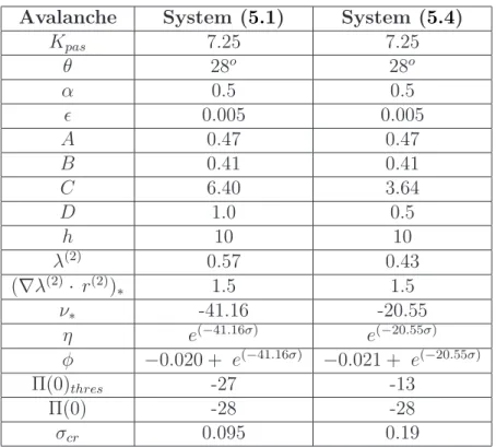
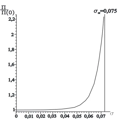
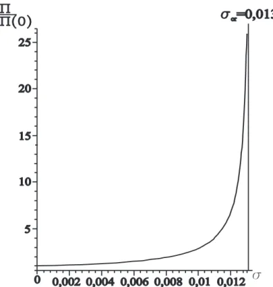
4 The Iverson and Denlinger model 39 5 A model for two flows classes 50 5.1 Weak discontinuity propagation in a constant state . . . 55
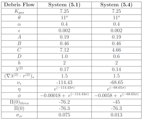
5.1.1 Some geophysical mass flows . . . 59
6 The two-fluid model 71 6.1 The one dimensional case . . . 81
6.1.1 Eigenvalues . . . 83
6.1.2 Some geophysical mass flows . . . 84
6.1.3 Approximate computations of λi . . . 89
6.1.4 Eigenvectors . . . 91
6.2 Weak discontinuity propagation in a constant state . . . 92
Introduction
The increase, in the past few decades, of the phenomena of intense transport of geophysical mass flows, pushed the technical and scientific community in face of the heavy responsibility to effectively protect people, man-made structures, and the economic activities of affected areas. Typical examples of these dangerous and destructive natural phenomena are landslides, snow avalanches, pyroclastic flows, debris flows that are driven down a slope under the action of gravity ([1]-[13]).
These gravity-driven flows, characterized by a mixture of soil, rocks and water, are often originated by sediments of natural deposits, mobilized of a considerable quantity of fluid and resulting in the formation of huge floods of sediments that are propagated with elevated speed. The characteristics of the flow depend on the rheology of dry granular flows and of the amount of fluid that is added, characterizing the mechanism of initiation along the streams listed first ([14]-[28].
Following the celebrated paper of Savage and Hutter [29], in the last two decades great progresses have been made in the mathematical and numerical modeling of granular geophysical flows by means of depth-averaged or thin layer models, which are based on the small aspect ratio of typical flows (small characteristic flow depth H compared to the characteristic flow length L). The study of Savage and Hutter was concerned with the one-dimensional motion of a relatively thin layer of a dry granular material along a slope. They started from the classical Saint-Venant system [30]:
∂th + ∂x(hu) = 0,
(1) ∂t(hu) + ∂x(hu2+ 12gh2) + hg∂xz(x) = 0
that has been widely used to model single-phase flows in one space dimension. In (1) h denotes the height of the material, u the velocity in the direction parallel to the bed, g the gravity constant. The influence of the topography enters through the function z(x) which is the altitude of the relief and it is assumed that ∂xz is small.
Savage and Hutter, modifying the Saint Venant equations, introduced a model which is still one-dimensional but take into account the curvature of the terrain at least when small. Both systems are hyperbolic and posses a convex entropy.
Eventually their approach has been followed and generalized by several authors which studied a bidimensional model but began to consider a complex basal topography ([31]-[38]). Even the extension to multidimensions of the Saint-Venant system is obvious, however it is valid only for almost flat topog-raphy, thus not relevant for debris avalanches in particular. Unfortunately the extension to several dimensions of the Savage-Hutter model appears to be far from trivial. The first attempt has been made by Gray, Wieland and Hutter [34], they assumed that the topography has large variation only in one direction, while it is essentially flat in the other direction. Later, see [39] and [40], Hutter and Pudasaini introduced a model for avalanches in arbitrarily curved channels.
It is worthwhile stressing that a considerable part of the literature on debris flow modeling, from the early studies to the most recent ones is de-voted to single-phase dry granular masses. Single-phase models are, however, limited in the simulation of the complex behavior of debris flows. As Hutter points out in [41] this is mainly due to neglecting the effects of the interstitial fluid. The effects of pore pressure on the fluidization of a solid-fluid mixture is often necessary for an accurate description of debris flows mechanics. In fact the interaction forces between solid grains and interstitial fluid influence not only the rheological behavior of the moving mass but also may play an important role in deformation processes, flow mobility and run-out. It is possible to find examples going from dry rock avalanches, in which pore fluid influence may be negligible, to liquid-saturated debris flows and gas-charged pyroclastic flows, in which fluids may enhance bulk mobility.
In order to take into account intergranular fluid effects in the flowing material Iverson [42] and Iverson and Denlinger [35], [43] suggested a new model by developing a depth averaged solid-fluid mixture theory based on the simplifying assumptions of constant porosity (fluid volume fraction) and equality of fluid velocity to solid velocity. In these models the flow is de-scribed by a set of balance equations for the mass and for the momentum of the mixture, which formally appears as a single-phase model with a stress term accounting for contributions from the two constituents. This mixture formulation lacks an inherent description of the pore fluid motion and the model needs to be supplemented with some specification of the pore fluid pressure evolution. In particular, the Iverson and Denlinger model extended the modeling to two dimensions, and included several refinements to the equations. Moreover, they postulate an advection-diffusion equation for the
fluid pressure, allowing for changes in the pressure in response to the move-ment of solid. Numerical applications of this model to laboratory avalanches and debris flume experiments are reported in [43].
The models of Savage and Hutter [29] and Iverson [42] have a very similar structure, this fact allows to formulate with appropriate positions a single model for two flows classes [44]. This particular model is hyperbolic, so for some experimental data, it is possible to write weak discontinuity evolution equation [45] and to evaluate the critical time, that is the instant when discontinuity amplitude becomes unbounded.
Making a significant progress with respect to the previous models, Pitman and Le [90] have recently introduced a novel depth-averaged two-phase model for debris flows and avalanches that contains mass and momentum balance equations for both the solid and fluid component. This implicitly provides equations for the velocities of both phases and for porosity. This model is tractable to describe unsteady and non uniform configurations encountered in real geophysical flows. In their work, the granular phase is described as a Coulomb material, and again, no dilatancy is present.
Moreover, in this thesis taking in consideration the Pitman and Le model and we study the partial differential equation system that tries to approach the range of scales and the complexity of the rheology for geological materials ([46], [47]). This system is a first order quasilinear system and we wonder if it is hyperbolic or not in order to look for propagation of weak discontinuities [45] and for further developments. Being the characteristic polynomial, in one space dimension, of degree four it is not trivial task to discuss about the reality of its zeros. Because of our interest are the application of this model to gravitational geophysical flows such as avalanches and debris flows, some experimental data are considered in order to compute the zeros of characteristic polynomial, to write weak discontinuity evolution equations and to evaluate the critical time.
The thesis is organized as follows. In section 1 the phenomenology of the geophysical mass flows is described. In section 2, the single-phase model of Savage and Hutter are shown. In section 3 the classical theory of mixtures are recalled, the derivation of a simple model for a Debris Flow Surges is shown and finally the ”hydraulic” model of Iverson is described. In section 4 the bi-phase model of Iverson and Denlinger is shown. In section 5 ”a model for two flows classes” is formulated and the propagation of weak discontinuities is studied. Finally, in section 6 the derivation of the two fluid model of Pitman and Le is shown, the hyperbolicity is discussed and the propagation of weak discontinuities is studied. In the last section conclusion are given.
Chapter 1
Phenomenology
1.1
Classification of the phenomena of mass
flows
The phenomena of instability of a slope are mainly due to factors directly related to the geometric shape of the slope, to the geological and geotechni-cal properties of earth and rocks involved in the process, and finally to the hydraulic characteristic of the site. These factors are extremely variable in time and space determine how the kinematics of breaking.
The apparent complexity of the phenomena has given rise to a large num-ber of classifications, in which we tried to group events according to the seemingly common material, the morphology of the deposit and the type of motion. However, as regards the casting of both land, both detritus, fast or slow with fluid consisting of water alone, alone by air or air-water mixture, were considered more significant that proposed by Varnes [48] on the phe-nomena of flow within mass motion, and descriptions of different types of motion of debris seconds Hutchinson ([49]-[51]).
The classification of Varnes [48] is the most complete and has become, especially from the engineering point of view, the most widely used reference for the terminology of mass motions. It uses as discriminatory elements, the type of motion derived from geometric and kinematic characteristics, and the type of material involved in the movement itself:
• type motion: collapse, overturning, rotational and passed slips, expand-ing side, castexpand-ings and complex motions.
• type material: the rock in place, coarse detritus, fine-grained soils. Varnes introduces the cast, starting from the observation that many examples of motions of slopes can not be classified as structural collapse, overturning or
slipping, and that in many cases the speed of distribution of mass in motion seems that of a viscous fluid. He considers two main types of flows: the flows in the rocks and streams of debris and soil.
The classification of Hutchinson [51] divides the movement of debris that looked like a stream into 4 types, showing that essentially differ in their mechanism of propagation ([52]-[64]).
• Mudslide. Are characterized by slow motions of debris accumulated in a clay matrix, mainly consisting of slips rather than flow.
• Debris flows. These flows fast or very fast debris and mixed with wa-ter are characwa-teristic phenomena of instability of the mountain slopes, where water leakage sudden supplied by rain or melting snow, can mo-bilize coperture detrital.
• Flowslides. Are characterized by a sudden collapse and from the wide one and rapids propagation of a mass of granular material or detrital after an external cause. Having the material a loose structure or high porosity, following the trouble, the collapse is had with partial total transfer of the overload on the fluid of porosity and therefore the gen-eration of an excess of pressure is had. The pore fluid usually consists of water, but in some cases it may be gas.
• Sturzstrom. This is true ”pattern of debris” that affect large vol-umes, with values of high-speed. The movement of sturzstrom depends on the turbolent granular flow, with a necessary tension dispersive in normal direction to the flow furnished by the transfer of momentum between the grains that collide and not by the presence of a liquid or gaseous fluid. There is therefore a fundamental difference between the behavior of sturzstrom and flowslides because, in addition to the different volumes involved, in the first ones the physical trial is tied up to the quantity of motion transferred through the collisions among wheats, while in the seconds it is essentially a phenomenon of impact liquefaction.
1.2
Physical characteristics of mass flows
The mass flows consists of detritus from mixtures consisting of air, water, colloidal suspensions of clay minerals, solid grains of various sizes (from sand to the blocks) in different proportions.
These phenomena of instability, typical of mountain slopes, are mobilized in connection with flooding and propagate downstream with speeds that can reach a few tens of meters per second. Flash floods gravitated in which the material undergoes a state of tension ring is unable to resist distortion and flows like a viscous fluid.
The main physical characteristics of the mass flows are: granulometry, speed and gradient.
1.2.1
Granulometry
The geological deposits which arise from the mass flows are not usually strat-ified and multi-class grain. The examination of the grading curve of some debris that have been casting motions [51] allows to put in evidence a break-down of the material that extends from the clay, the pebbles, the blocks. The percentage of each class may vary from one deposit to another and within a deposit.
The mass flows are, in fact, characterized by several phases of movement: a flow of material consists of mainly coarse elements are generally followed phases of fluidder flow.
1.2.2
Speed
The danger of Geophysical mass flows is closely linked to high speed with which these phenomena occur, since the speed between 0,5 m/s and 10 m/s. The differences between the values of velocity may be due to granuloma-try material affected, to the geomegranuloma-try of the channel and therefore to the inclination, the size and morphology of the area concerned.
1.2.3
Slopes
Although the mass flows originate on very inclined slopes, however, are char-acterized by the ability to move up inclines very weak. The ranges of observed slopes vary between 2% and 32%.
1.3
Mechanisms of initiation, propagation and
arrest of mass flows
A comprehensive study of physical processes in question should also consider the phase of initiation, as well as the maintenance of the phenomenon.
The formation of mass flow can in general due to the simultaneous occur-rence of the following three conditions:
1. the presence of detrital material (storage, layer, etc.);
2. intake of fluid (water, mud, etc..) sufficient for the mobilization of the material;
3. a slope of adequate fund.
In a mass flow can refer to two typical sources of material constituent, in percentage as:
• material accumulated and deposited in streams, from the sides, by the erosive action on the rocks, etc..
• material originated from erosive events concurrent with the occurrence of detrital casting.
The flow are mainly caused by events of particularly intense rainfall or sudden dissolution of the phenomena of glaciers due to sudden variations. Sometimes there may be a result of volcanic phenomena or as a result of landslides caused by earthquakes accompanied by surface water.
In such cases, the shear direction parallel to the slope increases with the degree of saturation, while the shear strength decreases with the increase in interstitial pression. The rupture occurs when cutting the shear active reaches the shear strength available. After the break, the unstable mass is moving, in some cases, very slowly and travels short distances, in other cases, however, is transformed into flow of detritus, reaching very high speeds and driving long distances.
Tubino and Seminara [65] have identified 4 different types of ignition of mass flows:
1. flow generated by the mobilization of debris deposited in the bed of streams, following the surface currents produced by heavy rainfall or thawing;
2. flow originated from the collapse of a slope, with subsequent transfor-mation of the landslide in detrital casting;
3. flow originated from the collapse of a natural dam, produced by the occlusion of a stream following a landslide the previous event;
4. flow produced by the fluidized immediate constituent of the material a landslide, due to the presence of an abundant surface current.
The mechanisms for generation of type 1, 3 and 4 are characterized, although with different modalities, from a flow of water in the form of tracking that is the cause of the phenomenon of instability. The mechanism of type 2 is, however, fundamentally different in that, to produce the phenomenon of instability, it is necessary that it is delivering the interstitial overpressure inside the material, leading to liquefazio with.
The classification proposed by Seminara and Tubino [65] reflects, besides, substantial differences in response times of the phenomenon: the time inter-val between the phenomenon and not trigger the occurrence of debris flow shows the hour-days in the case castings caused by landslides or slope failure, and stroke is reduced to the order of minutes-hours in the case of castings produced by the mobilization of deposits in the streams. In particular move-ment is very rapid in the case of non-saturated layers on high slopes.
The main characteristics of the debris on the move are:
• erosive capacity is particularly high during the initiation and develop-ment, during which the front of material thickens incorporating large, but much reduced in the subsequent propagation phase, during which the casting is characterized by a front face, where the sediments of greater dimensions are assembled, and an opposite rear end of the ma-trix;
• impact strength: due to the size of the granules of the front face (caus-ing major damage).
I can stop debris flows naturally and the effect of artificially drawn structures suitable for this purpose.
Experimentally it was observed that the debris flows deposited in plains or mountain gorges where the slope of the fund is reduced to values which can not exceed 3o. Generally, however, arrested at the mouth of a river or at
the apex of a cone.
In cases of non-stop the width of the current debris flow increases slightly and it has side storage with the formation of natural levees on both sides.
Chapter 2
The Savage-Hutter model
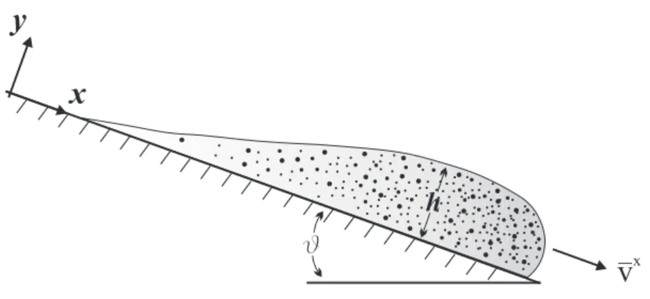
The Savage-Hutter model is a depth averaged dynamical model of a finite volume of cohesionless granular material in two dimensions released from rest on rough inclines. It takes into account the assumptions of density preserving (incompressibility), of a dry Coulomb-like friction law with bed friction angle σ, of shallowness of the flow with small topographic curvatures and finally the assumption of nearly uniform velocity profile through the flow depth.
Depth averaging the equations of conservation of mass and momentum yielding a tractable model of hyperbolic equations, reminiscent of the non-linear shallow-water equations. The granular mass is treated as a continuum along a slowly varying bottom profile with thickness, in which consider free surface flow and density not variable.
Mass and momentum balance equations for the incompressible model are written as ∇ · (ρsv) = 0, ρs(∂ tv + (v · ∇)v) = −∇ · Ts+ ρsg, (2.1)
where ρs is the constant density, v is the velocity vector, Ts is the solid
stress tensor and g the gravity acceleration.
The flow considered is represented in two-dimensional Cartesian coordi-nate system with x is the downslope direction and z the normal direction (see figure 2.1).
The equations of the system (2.1) in these coordinates system become:
vx x+ vzz = 0, ρs(gvtx+ vxvxx+ vzvxz) = ρsgsin(θ) − Txsxx− Tzsxz+, ρs(vz t + vxvxz+ vzvzz) = −ρsgcos(θ) − Txsxz− Tzszz, (2.2)
[H] [L] n F (x,t)=0s F (x)= 0 b Rear margin Longitudinal velocity Front margin y x
Fig. 2.1: Sketch of the geometry of a finite mass of granular material moving along a curved rigid bed showing definitions of the free surface given by Fh(x, z, t) = 0 and the equation of the bed Fb(x, z, t) = 0. Also indicated
are the scales [L] and [H] for the spread and maximum height.
where θ is the angle that the base of the mass flow makes with the hori-zontal, consequently sin(θ) and cos(θ) are the local components of gravity.
Boundary conditions at the upper free surface are two. First is the fol-lowing stress free condition:
Ts
· n = 0, (2.3)
where n is the exterior unit normal vector. The second boundary condition that in water wave problem is known as kinematic condition, is expressed by a function F , which is Fh(x, z, t) = 0 to indicate the position of the free
surface, then the further condition becomes:
Fth+ ∇Fh· v = 0, (2.4)
where the subscript t denotes the derivative with respect to the time. Instead, at the base the expression Fb(x, z) = 0 indicates the tangency of the flow,
that must satisfy the following condition:
v · n = 0. (2.5)
Furthermore, the boundary condition at the base satisfy the a sliding friction law, which expresses the proportionality between the shear traction S and the normal stress N as follows:
S = ±Ntang(φbed), (2.6)
where φbed is the basal friction angle and the sign is given by the direction of
the sliding velocity. With S = n · Ts − n(n · Ts · n), (2.7) and N = n · Ts· n, (2.8)
the two boundary conditions at the base (Fb(x, z) = 0) becomes: v · n = 0, n · Ts − n(n · Ts · n) = − vs |vs| ! (n · Ts · n)tang(φbed), (2.9)
where vs is the sliding velocity relative to the stationary bed.
The system of equations (2.1) is put in a non dimensional form by using the following scaling transformation:
(x, z, t) = L " ˜ x,H Lz,˜ L g ! 1 2t˜ # , (vx, uz) = (gL)1 2 v˜x,H Lv˜ z ! , Ts = ρsgH ˜Ts, (2.10)
where H is the characteristic thickness in the z-direction and L is the char-acteristic flow length in the x direction. Moreover, are specialized the free surface and the bed by z = h(x, t) and z = b(x), so that when h and b are scaled by H obtained: h(x, t) = H[˜h(˜x, ˜t)], b(x) = H[˜b(˜x)]. (2.11)
Consistent with the assumption of slow variation of the bed and the free surface, take ˜h and ˜b, as well as ∂˜h
∂ ˜x and ∂˜b
∂ ˜x to be order-unity functions. Moreover, introducing the term ǫ = H
L << 1, we can assert that the functions listed above are of order ǫ.
From eqn. (2.1) with scaling transformation (2.10), by dropping tilde and dividing each term by ρsg, we get the following three scalar equations written
in component form: vx x + vzz = 0, vx t + vxvxx+ vzvxz = −ǫTxsxx− Tzsxz+ sin(θ), ǫ(vz t + vxvxz+ vzvzz) = −ǫTxsxz − Tzszz − cos(θ), (2.12)
Putting ǫ = 0 in the z-momentum equation we obtain the following litho-static equilibrium equation:
Tzszz = −cos(θ). (2.13)
Instead, taking ǫ = 0 in the x-momentum equation, should neglect the lon-gitudinal stress tensor ǫTsxx
x , but unlike of the transverse stress tensor ǫTxsxz,
is sufficiently large to be retained.
The final procedure to simplify the x-momentum equation is the depth-average, which is integration in z, from the basal surface z = b(x) to the upper free surface z = h(x, t). Moreover, using the continuity equation and the Leibnitz’s rule, interchanging integrations and differentiations, the equation becomes: ∂ ∂t Z h b v xdz + ∂ ∂x Z h b v x2 dz − " vx ∂h ∂t + v x ∂ ∂t − v z !# z=h(x,t) + + " vx vx∂b ∂x − v z !# z=b(x) = sin(θ)(h − b) − T|z=h(x,t)sxz + T|z=b(x)sxz + −ǫ " ∂ ∂x Z h b T szz dy − T|z=h(x,t)szz ∂h ∂x + T szz |z=b(x) ∂b ∂x # (2.14)
Applying the boundary conditions at the free surface and the base, in the latter equation many terms are simplified. Moreover, the equation (2.14)
incorporates the following kinematic boundary conditions: ∂h ∂t + v x∂ ∂t − v z at z = h(x, t), vx∂b ∂x − v z at z = b(x), (2.15)
These conditions include the assumption that the surface of the flow of ma-terial is free of the stress, then consider:
Tsxz = Tsxx = Tszz = 0 at z = h(x, t), (2.16)
The equation (2.14) with the use of (2.15) and (2.16) simplifies and becomes: ∂ ∂t Z h b v xdz + ∂ ∂x Z h b v x2 dz = sin(θ)(h − b) + sin(θ)T|z=b(x)sxz + −ǫcos(θ) " ∂ ∂x Z h b T szzdy + Tszz |z=b(x) ∂b ∂x # . (2.17) Moreover, the depth-averaged velocities and normal stresses are defined as follows: vx = 1 h − b Z h b v xdz, (2.18) Tsxx = 1 h − b Z h b T sxxdz, (2.19) Tszz = 1 h − b Z h b T szzdz, (2.20) vx2 = 1 h − b Z h b αv x2 (h − b)dz, (2.21)
The term α in (2.21) indicates that if its value differs from unit, the velocity profile deviates from uniformity. Then, a value of α = 1 indicates a uniform profile and that the mass flow moves slipping on the base, with no differential shear. In this case the active shear zone is confined to a thin basal layer and the velocity profile is blunt [66].
Instead, if you do not slip on the base and the shear is all differential, the speed profile is parabolic and takes α = 6
Therefore assume a value of α ≈ 1 represents a good approximation, since it does not introduce a large errors.
With the shallowness assumption the non-dimensional form of the Coulomb sliding law (2.15) becomes
Tsxz = −sgn(vx)Tszzcot(θ) tan(φ
bed) at z = b(x). (2.22)
Assuming that the constitutive behavior of the material can be described by a simple Mohr-Coulomb yield criterion. By having postulated that the Coulomb constitutive relation for the material, is a nonlinear relation among the components of the solid tensor stress. Full reports expressing the Coulomb law are very complex to be used in Savage-Hutter derivation, because they yield the mass and momentum balance laws linearly ill-posed, then make the simplifications in the relations to be taken. However, it is based upon the results of shear cell and chute flow tests, and explanations of and jus-tifications for this assumption are given in considerable detail in [67]. The Mohr-Coulomb yield criterion for a cohesionless material with an internal friction angle ϕ, expresses the alignment between the shear stress and the normal stress, by the following relation:
Tsxz = Tszztan(ϕ), (2.23)
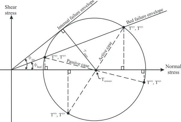
This is shown schematically in terms of a standard Mohr-diagram (see figure
2.2) for the case of a constant internal friction angle and a constant bed friction angle φbed.
At the bed , the normal stress Tszz and the shear stress Tsxz must be such
that they lie on the wall yield line as shown. Note that two possible Mohr circles can be drawn through the point corresponding to the (Tszz, Tsxz) stress
state. That one corresponding to a larger value of the normal stress Tsxx (i.e.
Tsxx > Tszz) we associate the passive state of stress (to use the common soil
mechanics terminology) and the other we associate with the active state of stress. An earth pressure relation expresses the proportionality between the diagonal stress components, as follows:
Tsxx = Kact/pasTszz, (2.24)
where Kact/pas is the earth pressure coefficient, determined by the equation:
Kact/pas = 21 ∓ [1 − cos 2(φ
int)[1 + tan2(φbed)]]1/2
cos2(φ
int) − 1,
(2.25) with φint is the internal friction angle. The sign ∓ depends on whether
Shear stress Normal stress Inte rnal fa ilure enve lope Bedfailu re envelo pe Activ eca se Passive case Fint Fbed T ,syy Tsyx T ,syy Tsyx T ,sxx Tsyx T ,sxx Tsyx Ts(mean) t ma x
Fig. 2.2: Mohr stress circle and Coulomb failure envelopes for a granular material that is simultaneously slipping along a bed and failing internally. The radius of the stress circle defines the maximum internal shear stress. with - sign) or compressed (”passive” coefficient ∂v/∂x < 0, with + sign) in
the direction parallel to the bed.
The relation (2.17) with (2.18)-(2.24) becomes: [(h − b)vx]
t+ [α(h − b)vx2]x= sin(θ)(h − b) +
−ǫcos(θ)Kact/pas{[(h − b)Tszz]x+ Tszzbx} +
−cos(θ)sgn(vx)Tszztan(φ
bed). (2.26)
From (2.13) after integration and taking account of the zero pressure condi-tion at the free surface obtained the following overburden pressure:
Tszz = h(x, t) − b(x) =bh(x, t) (2.27)
and still has:
b
hTszz = 1
2[h(x, t) − b(x)] = 1
So the relation (2.26) with (2.27) and (2.28) becomes: [bhvx]
t+ [αbhvx2]x = sin(θ)h − ǫcos(θ)Kb act/pas{bh2x+bhbx} +
−cos(θ)sgn(vx) tan(φ
bed)bh. (2.29)
Finally, after integration of the first equation of the system (2.2) over the depth and use the kinematic boundary conditions at the free surface and at the base, the continuity equation becomes:
b
ht+ (bhvx)x = 0. (2.30)
The relation (2.31) using the (2.30) is simplified as: vx
t+ vxvxx = sin(θ) − ǫcos(θ)Kact/pas{hbx+ bx} +
−sgn(vx)cos(θ) tan(φ
bed), (2.31)
taking a value of α = 1.
Equations (2.30) and (2.31) comprise a system of two partial differential equations for the profile bh(x, t) and the transversely averaged velocity vx.
Provided the internal angle of friction ϕ, the basal friction angle φbed, and
the basal geometry (through the angle θ and the function b(x) are known. The evolution in time of both h(x, t) and vb x can be determined if an initial
profile and a velocity distribution
h(x, 0) = h0(x), vx(x, 0) = vx 0(x), (2.32) are prescribed. In particular, for the motion of an avalanche along a planar bed the authors may set b = 0 and replace bh by h. So the considerations of the present model will be restricted to this case, and the system become:
ht+ (hvx)x = 0, vx
t + vxvxx= sin(θ) − sgn(vx)cos(θ) tan(φbed) − βhx,
(2.33) where we have omitted the over bars for simplicity and
β = ǫKact/pascos(θ) (2.34)
is a small constant. Boundary conditions which must imposed upon the system (5.8) are: h(x, t) = hF(t) at x = xF(t), h(x, t) = hR(t) at x = xR(t), (2.35)
with x = xF(t) and x = xR(t) denoting the front and rear margins
respec-tively, while hF(t) and hR(t) are prescribed functions of time. Note that
hF(t) = hR(t) = 0 are obvious choices, but cliffs are also possible.
Finally, we mention that the margin velocities are given by:
uF = dxdtF, uR= dxdtR. (2.36)
Chapter 3
The Iverson model
In an extensive review of debris flows, Iverson [42] presented a thin layer model for a mixture of granular material and interstitial fluid in one spatial dimension.
Before dealing with the analysis of the model described by Iverson, we think it is useful to show a short review of the equations governing the theory of mixtures, which underlie this model.
The governing equations for a debris flow can be obtained from established theory of continuous mixtures [68]. Equations are formulated separately, even if strongly coupled, they describe the balance of conservation of mass and momentum, respectively for solid and liquid constituents of a debris flow. In addition, as it is usual for the classical theory of mixtures, these equations both for solid and liquid are assumed to be valued simultaneously be all positions.
It usually, these equations for the solid and the liquid are assumed to be applied simultaneously to all positions. One could also formulate an equation of balance of moment of momentum, but this is not necessary since it is assumed that the stress tensor is symmetric. Similarly, the thermodynamic energy balance is made redundant, because it is assumed that the mixture is isothermal. The mixture theory mass conservation equations for the solid and fluid constituents are, respectively:
∂(ρsϕ) ∂t + ∇·(ρ sϕvs) = ms, (3.1) ∂[ρf(1 − ϕ)] ∂t + ∇·[ρ f(1 − ϕ)vf) = mf, (3.2)
where ϕ is the solid volume fraction, vs and vf are the solid and fluid
ve-locities and and ms and mf are the respective rates of solid and fluid mass
addition, per unit volume.
As the material of the debris flow is saturated, the volume fractions of solid and fluid must satisfy the condition of saturation. As a result, the equations (3.1) and (3.2) are coupled, and their sum gives an equivalent equation of conservation of the total mass of the mixture:
∂ρ
∂t + ∇·(ρv) = m
s+ mf, (3.3)
where the total mass density of the mixture ρ and the barycentric velocity v, are defined by:
ρ = ϕ + ρf(1 − ϕ) (3.4)
v = ρ
sϕvs+ ρf(1 − ϕ)vf
ρ (3.5)
Now, we consider the special case of conservation of mass, in which the variations of mass are zero (ms = mf = 0) and the solid and fluid constituents
are individually incompressible.
By summing (3.1) and (3.2) we get the alternative forms of mass balance:
∇ · (1 − ϕ)(vf − vs) + ∇·vs = 0, (3.6)
∇·v = 0, (3.7)
After having substituted the fluid specific discharge, q = (1 − ϕ)(vf − vs),
in the equation (3.6) we get the standard form of the equation of continuity for deforming porous media subject to quasistatic [69] or inertial motion [70]. In this way it is exploited the analogy between the mixtures of debris flow and porous media. Finally, the (3.7) represents the standard continuity equation for an incompressible, single-phase continuum.
In general, from the theory of mixtures, the momentum balance equation of the solid and fluid phase are, respectively:
ρsϕ[∂vs/∂t + vs·∇vs] = ∇·Ts+ ρsϕg + f − msvs, (3.8)
ρf(1 − ϕ)[∂vf/∂t + vf
·∇vf
] = ∇·Tf + ρf
(1 − ϕ)g − f − mfvf, (3.9)
where g is gravitational acceleration, Ts and Tf are the solid phase and
fluid phase stress tensors, respectively, and f is the interaction force per unit volume that results from momentum exchange between the solid and fluid constituents. Sign conventions define normal stresses as positive in tension and f as positive when it acts on the solid.
The last term of (3.8) and (3.9) arises from the nonzero terms on the right-hand sides of (3.1) and (3.2) and account for momentum change due to mass change. However, they do not account for forces that enable mass change, and they assume that mass enters or leaves with zero momentum.
By adding the (3.8) and (3.9), and considering the special case with (ms=
mf = 0), the mixture is obtained, the equation of conservation of momentum:
ρ[∂v/∂t + v · ∇v] = ∇·(Ts+ Tf + ˆT) + ρg, (3.10)
in which
ˆ
T = ρsϕ(vs− v)(vs− v) − ρf(1 − ϕ)(vf − v)(vf − v), (3.11) is a contribution to the stress of the mixture, resulting from the motion of fluid and solid constituents.
ˆ
T brings in (3.10), the convective acceleration terms of the mixture, given by v·∇v.
It shows in a two-phase mixture (debris flow), represented as a single material, the stresses are more complex than those obtained by adding the stress of the solid and fluid Ts+ Tf.
Finally we can observe that by excluding ˆT, the equation (3.10) assuming the form of a single-phase continuum balance equation.
The basic equations of the mixture’s theory (3.1-3.10) compared with those for single phase, show three significant advantages with respect to com-parable single-phase equations:
1. they represent explicitly the volume fractions of solid, of fluid and changes in mass, allowing them to show the various compositions or evolution of a debris flow;
2. they include separately the stress tensor for the solid and fluid, which have a direct physical meaning.
On the contrary, in the single-phase models of the stress tensor that amalgamates the effects of solids and fluids and their interactions. This formulation of stress, to describe the rheology of the mixture may need the use of many parameters poorly constrained.
3. the momentum mixture equations contain explicit solid-fluid interac-tion force. Such a force is missing in the single-phase models, that include they effect in the mixed stress tensor.
Since the solid-fluid interactions vary from point to point within a de-bris flow, playing an important role physical, it is necessary to introduce an explicit representation of their effects.
3.1
A simple model for a Debris Flow Surges
There are two phenomena that characterize the unstable motion and non-uniform of a debris flow:
1. In a debris flow, the pressure of the fluid, which can not exists in a con-stant and uniform motion, is significantly greater than the hydrostatic pressure, thus increasing the efficiency of the flow. The significant in-fluence of pore pressure on the mechanics of debris flow can be molded easily by introducing the actual pore pressure in a specially formulated hydraulic model (as we will see in Section 3.1).
2. The debris flow, move as a surge or series of surges, in which coarse-grained heads that lack high fluid pressure restrict the downslope mo-tion of finer-grained debris that may be nearly liquefied by high fluid pressure.
The concentration of coarse material (clasts) at the surge heads, means that the hydraulic diffusivity is higher than in the main part of materials of de-bris flow. This is because the heads of the pulses appear unsaturated and exhibit small or no pore fluid pressure. The interaction of the surge heads with the almost liquid material, plays a key role in the determination of the unstable and non-uniform motion and limit the expansion of the debris flow. The remaining parts of the flow almost liquefied provide a small frictional resistance to motion, unlike the surge heads.
A rigorous evaluation of the interaction between the dry surge heads with the material liquefied almost requires the numerical analysis of the motion unstable and non-uniform flow.
However a simple analysis of steady-state, provides a framework for under-standing the problem and interpretation of numerical results. Such analysis ([71]-[73]), assumes that the surge heads acts as a rigid body shifted, with resistance at the base of Coulomb and pushed back by a mass completely liquefied.
This analysis ignores other forms of resistance, considering only those associated with internal deformation, ignore all the inertial effects and time-dependent, whereas the evolution of the shape of the flow and finally, ignore the multi-dimensional effects that can not be represented with a balance one-dimensional forces.
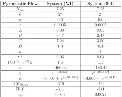
We consider here, the simple model of the pulse of a debris flow, shown in Figure 3.1.
h
q
l
Liquid
Solid
Fig. 3.1: Schematic vertical cross section of the rigid body model of a debris-flow surge, with geometric parameters defined ([71], [72]).
The surge head has a triangular cross-sectional shape with height h equal to the debris flow thickness measured normal to the slope. The length l of the surge head is measured parallel to the slope.
The mass of the surge head is then 12ρhlw , where ρh is the bulk density
of the head and w is its breadth normal to the plane of the page.
The basal shear force τ and normal force σ due to the action of gravity on the head are simply:
τ = 1
2ρhghlw sin θ, (3.12)
and
σ = 1
2ρhghlw cos θ, (3.13)
The slope basal parallel Coulomb resistance, sliding of the head, is de-scribed by −σ tan φ, and the slope parallel force of the liquefied debris flow body pushing against the upslope face of the head is described by 12ρbgh2lw cos θ,
where ρb is the density of the liquefied body. This expression assumes that
Steady motion of the head then requires to be zero the sum of the slope parallel forces acting on the head:
1 2ρhghlw sin θ − 1 2ρhghlw cos θ + 1 2ρbgh 2lw cos θ = 0, (3.14)
Combining the terms of (3.14) [72]we get: h
l = ρh
ρb(tan φ − tan θ).
(3.15)
Moreover, if we assume ρh ≈ ρb, for reasonable approximation debris flow,
the (3.15) can be expressed as:
h
l = (tan φ − tan θ). (3.16)
The quantitative predictions of (3.15) and (3.16) must be interpreted with great caution because of several factors neglected in the analysis. However, they provide some insight for the interpretation of the behavior of debris flow and to predict more elaborate models.
(3.16) shows that on steep slopes, when θ → φ, we obtain h l → 0.
This implies that the momentum tends to accelerate on the steep slope, unless the length of the head is much larger than its height.
Furthermore, in addition, pulses with identical values of l, rise height h larger and with greater acceleration, overtaking the smaller pulses.
Instead, for small angles of slope, when θ → 0, (3.16) becomes hl = tan φ, this implies that the pulse will slow down and stop, unless, which requires that the heads of the pulses are short and steep.
Typically an angle of friction φ → 30o is sufficient to stop the movement,
in fact, the length exceeds the value so that the frictional resistance of the head of the pulse is capable of stopping the movement of the flow.
A more realistic assessment of the role of the head of the pulse requires a model such as that described in the following section.
3.2
Hydraulic modeling and prediction of
de-bris flow motion
This model formulated by Iverson [42], known as ”hydraulic model”, uses the simplifications of the hydraulics theory and is one of the most refined for the prediction of unstable and non-uniform motion of a debris flow, and its limits of expansion and flooding.
In this model are still used of depth-averaged equations of motion. How-ever, are neglect some key physical phenomena, such as the rigorous treat-ment of the evolution of the granule temperature and non-hydrostatic pore pressure.
To account for debris flows variable composition, the possibility of bound-ary slip, and the mechanics of initiation and deposition as well as flow, the hydraulic model described here uses internal and basal friction angles and pore fluid viscosity to characterize flow resistance. This simplifies the rig-orous testing of the model because the values of the angles of friction and viscosity of the fluid can be measured independently rather than being cali-brated.
In fact, the calibration is a problem of debris flows because the transport mechanisms of the time and energy dissipation differ significantly depending on the type of event.
The mathematical formulation is based on the change of hydraulic theory for dry granular flows developed by Savage and Hutter [29].
To clarify the assumptions of hydraulic formulation we refer to the rela-tionships described in the theory of mixture.
A simpler form of the equations of momentum of the mixture (3.8) and (3.9), can be obtained by focusing attention on the motion of solids, and analyzing the motion of fluid in relation to that of solids. So, it is defined
that q
(1 − ϕ) = v
f
− vs.
where q is the specific discharge and (1 − ϕ) is the volume fraction of the fluid
Substituting this relation into the equation of momentum of the fluid, we get: ρf(1 − ϕ)[∂ ∂t q 1 − ϕ+ v s ! + q 1 − ϕ·∇ q 1 − ϕ+ v s ! + vs ·∇ q 1 − ϕ + v s ! = = ∇·Tf + ρf (1 − ϕ)g − f, (3.17)
Darcy’s law provides an estimate of the largest plausible q in (3.19) be-cause data show that hydraulic head gradients in debris flows commonly approach but seldom exceed liquefaction-inducing gradients, which roughly is equal 1. Thus the hydraulic conductivity, for example, provides a good es-timate of the maximum magnitude of q, and the conductivity rarely exceeds 0.01 m/s for debris flow materials. In contrast, vs typically exceeds 1 m/s.
By this rationale, vs generally exceeds q
1 − ϕ by more than an order of magnitude, then assuming
q 1 − ϕ << |v s | (3.18) the (3.19) becomes: ρf(1 − ϕ) " ∂vs ∂t + v s ·∇vs # = ∇·Tf + ρf(1 − ϕ)g − f, (3.19)
This equation implies that inertial forces affecting fluid motion are prac-tically indistinguishable from those affecting solid motion, except insofar as the fluid and solid masses per unit volume of mixture differ.
By adding (3.19) with (3.8), we obtain a simplified equation of momentum of the solid-fluid mixture:
ρ " ∂vs ∂t + v s ·∇vs # = ∇·(Ts+ Tf) + ρg, (3.20)
where ρ is the density of the mixture defined by (3.4), we also note that the solid-fluid interaction force f does not appear explicitly, but implicitly lies in the combination of solid-fluid stress tensor Ts+ Tf.
The assumption (3.18), produces a further simplification of the mass bal-ance equation (3.6), which reduces to the following form:
∇·vs = 0. (3.21)
The equations (3.20) and (3.21) are the equations governing the debris flow. They differ from the equations governing the motion of granular solids to a single-phase, because they involve the total mass density ρ of the mixture and the influence of the fluid stress Tf (implicitly considered in the equation
of momentum of the mixture).
We consider a two-dimensional flow through an infinitely wide planar surface, inclined at an angle θ to the horizontal, as shown in Figure 3.2.
h
v
xq
x
y
Fig. 3.2: Schematic vertical cross section of an unsteady, deforming debris flow surge moving down an inclined plane. The flow depth h and depth-averaged velocity vx vary as functions of x and t.
The equations (3.20) and (3.21) generalized to two spatial coordinates x and y become: ∂vx ∂x + ∂vy ∂y = 0, (3.22) ρ " ∂vx ∂t + vx ∂vx ∂x + vy ∂vy ∂y # = −∂T s xx ∂x − ∂Ts yz ∂y − ∂Tf xx ∂x + −∂T f yz ∂y + ρg sin θ, (3.23) ρ " ∂vy ∂t + vy ∂vy ∂y + vx ∂vy ∂x # = −∂T s yy ∂y − ∂Ts xy ∂x − ∂Tf yy ∂y + −∂T f xy ∂x + ρg cos θ, (3.24)
Since all velocities refer to the solid phase, we omitted the subscript s, also the speed of the x and y subscripts denote the Cartesian components parallel and normal to the inclined plane.
Sign conventions for stress components have been reversed so that com-pression and left-lateral shear are positive [29].
The subscripts denote the Cartesian components of the stress of the solid and fluid, the first subscript indicates the direction normal to the plane of ac-tion of components of stress, and the second subscript indicates the direcac-tion of action.
Finally, the subscripts (x, y) and (y, x) are interchangeable because it is assumed that the stress tensor is symmetric.
To normalize the equations (3.22-3.24), we introduce two scale lengths: L the characteristic length of flow in x direction, and H the characteristic height of flow in y direction.
Therefore, the parameter ǫ = H
L describes the ratio of these lengths of scale and is considered generally much smaller than 1.
Instead, the characteristic time scale is given by the free fall in the x direction (L/g)12, as the potential free fall is leading the movement of debris
flow.
These time and length scales in turn lead to different scales of speed, in x direction (Lg)12 and y direction ǫ(Lg)
1
2, and also imply that vx >> vy.
Finally, the scale of stress are the stress that existed on the basis of a constant flow and uniform height H, ρgH sin θ for shear stress and ρgH cos θ for normal stress and pore pressure.
In summary, using the following scaling transformation:
(x, y, t) = L(˜x,HLz, (˜ Lg)12t),˜ (vx, vy) = (gL)12(˜vx,H L˜v y), (Txx, Tyy) = ρsgH sin θ( ˜Txx, ˜Tyy) (Txy, Tyx) = ρsgH cos θ( ˜Txy, ˜Tyx) (3.25)
The system of equations (3.22-3.24) with scaling transformation (3.25), by dropping tilde, multiplying each term of (3.22) by (L/g)12, dividing each
term of (3.23) and (3.24) by ρg and taking the limit as ǫ → 0, we get the following
three scalar equations written in component form: ∂vx ∂x + ∂vy ∂y = 0, (3.26) ∂vx ∂t + vx ∂vx ∂x + vy ∂vy ∂y = sin θ " 1 −∂T s yz ∂y − ∂Tf yz ∂y # + +ǫ cos θ " − ∂T s xx ∂x − ∂Tf xx ∂x # , (3.27) 0 = cos θ " − 1 − ∂T s yy ∂y − ∂Tf yy ∂y # . (3.28)
These equations differ from governing equation of Savage and Hutter [29] only by including fluid stresses.
Equations (3.26-3.28) have two key properties:
1. The y direction momentum balance (3.28) has a simple form identical to that for steady, uniform flow; its integration shows that the total normal stress at any depth is simply the static stress ρg(h − y) cos θ. 2. The x direction momentum balance (3.27) includes longitudinal
nor-mal stress gradient terms preceded by the snor-mall parameter ǫ, which apparently indicates that such terms can be neglected.
However, as was explained by Savage and Hutter, neglect of longitudinal normal stress gradients is untenable because it produces a stress field identical to that for steady, uniform flow, which negates any hope of modeling surge-like motion.
The physical rationale for retaining this term becomes more apparent when the equations are integrated over the flow depth.
The final step in the simplification of the equations of government is to introduce the depth integration, which incorporates the assumptions with respect to stress and produces constitutive equations without explicit depen-dence on y.
The process is linear, but rather prolonged, then try to summarize the results easily. It includes repeated application of Leibniz’s rule for integrating derivatives and incorporates kinematic boundary conditions, which state that
the mass does not enter and exit the free surface (where y = h) and the bed (where y = 0), ∂h ∂t + vx ∂h ∂x − vy = 0 at y = (x, t) (3.29) vy = 0 at y = 0 (3.30)
It also involves the assumption that the debris flow surface is free of all stresses,
Txxs = Tyys = Txys = Txxf = Tyyf = Txyf = 0 at y = (x, t) (3.31) and it employs depth-averaged velocities and normal stresses defined by
vx = 1 h Z h 0 vxdy, (3.32) Ts xx = 1 h Z h 0 T s xxdy, (3.33) Ts yy = 1 h Z h 0 T s yydy, (3.34) Txxf = 1 h Z h 0 T f xxdy, (3.35) Tyyf = 1 h Z h 0 T f yydy, (3.36) v2 x = 1 h Z h 0 v 2 xdy = αv2x, (3.37)
The value of α in (3.37) [29], provides information on the deviation of the vertical velocity profile uniformity. If a debris flow moves only for basal slip, is applied 1.
For a description of the constitutive stress in (3.27), we use the simple relationship of Coulomb granular solids, in dimensionless form:
Txys = −sgn(vx)Tyys cot θ tan φbed/int, (3.38)
where φbed/int indicates the appropriate friction angle for bed slip or internal
deformation, sgn(vx) denotes the sign (+ or -) of (vx) and cot θ is introduced
because of the different scalings for shear and normal stress components. Finally, in (3.38) does not appear explicitly the effects of pore pressure, but implicitly, because the Ts
yyand Tyyf refer to (3.28). Thus as fluid pressures
Tf
yy grow in magnitude, the magnitudes of Tyys and Tyxs diminish.
Moreover, the Coulomb rule leads directly to the following expression of Ts
xx and Tyys obtained from classical Rankine [79] earth pressure theory:
Txxs = Kact/pasTyys , (3.39)
where Kact/pas is an earth pressure coefficient that has different values
de-pending on whether the flow is actively extending ∂vx ∂x > 0 ! or passively compressing ∂vx ∂x < 0 !
, and its expression presented without derivation by Savage and Hutter:
Kact/pas = 21 ∓ [1 − cos 2(φ
int)[1 + tan2(φbed)]]1/2
cos2(φ
int) − 1,
(3.40) where the sign ”-” applies to the active coefficient, and the sign ”+” applies to the passive.
Equations (3.26-3.40) provide all information necessary to complete the formulation of hydraulic equations.
Integration of equation (3.26) from y = 0 to y = h, with application of the kinematic boundary conditions (3.29-3.30) produces a depth-averaged mass conservation equation:
∂h ∂t +
∂hvx
∂x = 0. (3.41)
Integration of (3.28) from y = 0 to y = h yields a steady momentum balance in the y direction, which states that the sum of the nondimensional
solid and fluid stress balances the y component of the nondimensional total mixture weight
Tyys + Tyyf = h(x, t) − y. (3.42)
This in turn leads to nondimensional expressions for the total (solid plus fluid) normal stress at the bed and for the y direction depth-averaged total normal stress, Tyys + Tyyf = h, at y = 0 (3.43) Tsyy+ Tfyy = 1 h Z h 0 (h − y)dy = 1 2h. (3.44)
Integration of the normalized x direction momentum equation (3.27) from y = 0 to y = h, gives the following expression:
∂ ∂t(hvx) + ∂ ∂x(αhv 2 x) = h sin θ+
+(Tyx|y=0s ) sin θ + (Tyxf|y=0) sin θ+
−ǫ cos θ∂x∂ (hTsxx) − ǫ cos θ ∂ ∂x(hT
f
xx). (3.45)
Terms on the right-hand side of (3.45) can be interpreted as follows. The first term represents the gravitational driving stress. The second term repre-sents frictional resistance to slip at the base of the flow and can be evaluated by applying the Coulomb equation (3.38) and the normal stress equation (3.43) at the flow base
(Ts
yx|y=0) sin θ = −sgn(vx)(h − pbed) cos θ tan φbed (3.46)
where h − pbed is the nondimensional basal effective stress and φbed = Tyx|y=0f
is the nondimensional basal pore pressure.
The third term on the right-hand side of (3.45) represents flow resistance due to shear of the fluid at the flow base. It can be evaluated using Newton’s
law of viscosity [42], which yields (Tyx|y=0f ) sin θ = −(1 − ϕ)µ ∂vx ∂y ! |y=0 (3.47) where µ is the appropriate, nondimensional depth-averaged viscosity, given by
µ = h µ
ρgh2/gl1/2i. (3.48)
Application of (3.48) requires knowledge of the fluid velocity gradient at the bed, ∂vx
∂y
! |y=0
, which is generally unknown but can be obtained from estimates of the vertical velocity profile. The estimates are constrained by assuming no slip of fluid at the bed and a mean fluid velocity of vx.
For example, if the velocity profile is linear, then ∂vx ∂y
! |y=0
= vx
h. If the velocity profile is parabolic, then a simple analysis of laminar flow down an incline shows that ∂vx
∂y
! |y=0
= 3vx
h . If the velocity profile is blunt, with shear strongly concentrated near the bed, a good descriptor is ∂vx
∂y
! |y=0
= (n + 2)vx
h , where n = 1 indicates a parabolic profile and n > 1 indicates blunter profiles; this form is used below.
The fourth term on the right-hand side of (3.45) represents the longitu-dinal stress gradient due to interaction of solid grains. It can be evaluated using (3.39) and (3.44), yielding
− ǫ cos θ∂x∂ (hTsxx) = −ǫKact/pascos θ
∂ ∂x h2 2 − hT f yy ! . (3.49)
As is indicated by the presence of Tfyy in (3.49), the longitudinal solid stress gradient is mediated by fluid pressure.
The final term in (3.45) represents the longitudinal stress gradient due to the fluid pressure alone. Because fluid pressure is isotropic, it can be rewritten with Tfyy in place of Tfxx,
− ǫ cos θ ∂ ∂x(hT f xx) = −ǫKact/pascos θ ∂ ∂x h2 2 − hT f yy ! . (3.50)
The utility of (3.49) and (3.50) is enhanced by evaluating the integral (3.36) to calculate Tfyy for a condition in which the fluid pressure increases linearly from zero at the debris flow surface to a maximum of pbed at the bed
(a condition consistent with the hydraulic theory assumptions). Integration shows that we can write
∂hTfyy
∂x = h
pbed
∂x .
The final form of the x direction momentum equation results from in-corporating (3.41) and (3.46-3.50) in (3.45), assuming α = 1, collecting and canceling like terms, and dividing by h, which yields
∂vx ∂x + vx ∂vx ∂t = sin θ − sgn(vx) 1 − pbed h !
cos θ tan φbed+
−(1 − ϕ)µ(n + 2) vx h2
!
+
−ǫ cos θ∂x∂ [Kact/pas(h − pbed) + pbed]. (3.51)
Together, (3.51) and (3.41) form a set of two equations in two unknowns, vx(x, t) and h(x, t), which can be solved provided that the basal pore fluid
pressure pbed(x, t) and the necessary initial and boundary conditions are
spec-ified.
The need to specify rather than predict basal pore pressures is inherent to the hydraulic model; fluid pressure deviations from hydrostatic values result from velocity components normal to the bed, and neglect of such velocities in (3.28) precludes the possibility of predicting non hydrostatic pressures.
Thus inclusion of non hydrostatic pressures pbed(x, t) may seem to
contra-dict the hydraulic model assumptions. The inclusion is justified, however, on the grounds that the consolidation process responsible for generating non hy-drostatic fluid pressures typically operates on timescales substantially longer than the debris flow duration.
Thus as a first approximation, high pore pressures, once established, may be assumed to persist in debris flows, and pore pressures may be treated as parameters in hydraulic model calculations.
Inspection of the individual terms in (3.51) reveals how the hydraulic model encapsulates debris flow physics.
The inertial terms on the left-hand side of (3.51) show that both rigid body accelerations and convective accelerations may be important.
On the right-hand side of (3.51), if the first two terms are viewed in isolation, they depict a static balance of forces identical to that used in infi-nite slope stability analyses for cases in which there is zero cohesion and an arbitrary distribution of pore pressure [74]-[75].
If the last term on the right-hand side is included, this static force balance assumes a form comparable to that of two-dimensional slope stability analyses that use methods of slices, and in this case the interslice forces are represented by depth-averaged Rankine stresses.
Thus the model subsumes classical models of the statics of landslides with spatially varied pore pressures as a limiting case, which applies to incipient debris flow motion.
The third term on the right-hand side of (3.51) represents the effects of shear resistance due to fluid viscosity.
The motion of a frictionless but viscous mass is represented by the special case where φbed/int = 0 or, alternatively, pbed = h (in which case the mass is
completely liquefied by pore pressure).
The final term is perhaps the most interesting and important term in (3.2), for it describes the longitudinal stress variation that accompanies vari-ations in flow depth and surge-like motion.
The term shows that a great change in debris flow behavior occurs as pbed
ranges from 0 to h. If pbed = h and the sediment mass behaves like a liquid,
normal stresses are isotropic, equal to the static pressure, and independent of the local style of deformation. If pbed = 0 and the debris behaves like a
Coulomb solid, normal stresses are anisotropic, and the longitudinal normal stress depends strongly on whether the sediment mass is locally extending
∂vx ∂x > 0 ! or compressing ∂vx ∂x < 0 !
as it deforms and moves downslope. Consequently, the model predicts that strong local gradients in the lon-gitudinal normal stress can occur for two reasons: either the style of defor-mation changes locally from extending to compressing, or the pore pressure varies locally from high to low.
Thus, depending on the deformation style and pore pressure distribution, the model expressed by (3.41) and (3.51) can represent unsteady flow behav-ior that ranges from that of a granular avalanche, as modeled by Savage and Hutter [29]-[67], to that of a liquid surge, as modeled by Hunt [76].
Furthermore, the front of a fully developed debris flow may act like a compressing granular solid and support high lateral stresses, while the trailing flow acts more like a fluid.
This phenomenon explains how debris flow surges with steep snouts and gradually tapered tails can move downstream with only modest attenuation. The initial and boundary conditions used in conjunction with (3.41) and
(3.51) are identical to those described by Savage and Hutter [29].
The initial conditions specify the zero velocity and static geometry of the mass that mobilizes into a debris flow,
vx(x, 0) = 0 (3.52)
h(x, 0) = h0(x) (3.53)
Boundary conditions stipulate that the height of the deforming mass is zero at the front margin (x = xF) and rear margin (x = xR),
h(xF, t) = 0 (3.54)
h(xR, t) = 0 (3.55)
These zero-depth boundary conditions are connected to the velocities at the front and rear flow margins by the relations
vFx(x, 0) = dxF
dt (3.56)
vRx(x, 0) = dxR
dt (3.57)
Chapter 4
The Iverson and Denlinger
model
This model is a generalization of the depthaveraged, two-dimensional grain-fluid mixture model of Iverson [42], who in turn generalized the one-phase grain flow model of Savage and Hutter [29].
The new generalization yields depth-averaged mass and momentum bal-ance equations that describe finite masses of variably fluidized grain-fluid mixtures that move unsteadily across a threedimensional terrain, from initi-ation to deposition.
In generalizing to three spatial dimensions we address key physical issues concerning with preservation of frame invariance, symmetry of conjugate shear stresses, magnitudes of lateral forces, and distributions of pore fluid pressure.
Here, along the guidelines of the paper of Iverson and Denlinger [35] we consider the relevant equations for debris flow resulting from the theory of mixtures (see Section 3): :
∇·vs = 0. (4.1) ρ " ∂vs ∂t + v s ·∇vs # = ∇·(Ts+ Tf) + ρg, (4.2)
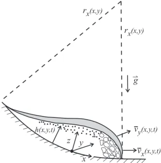
A key step in further simplifying the equations of motion involves depth averaging to eliminate explicit dependence on z which is the coordinate nor-mal to the bed.
Depth averaging requires decomposing the vector equations (4.1) and (4.2) into component equations in locally defined x, y, z orthogonal
direc-rx(x,y) rx(x,y) h(x,y,t) vy(x,y,t) vx(x,y,t) z y x g
Fig. 4.1: Schematic cut-away view of an unsteady flow down a curvilin-ear slope, illustrating the local coordinate system and dependent variables h(x, y, t), vx(x, y, t), vy(x, y, t) that describe depth-averaged flow. The x
com-ponent of bed curvature is specified by the local radius of curvature rx.
tions, then integrating each component equation from the base of the flow at z = 0 to the surface of the flow at z = h (see Figure 4.1).
The pertinent mathematical manipulations are rather lengthy, and we omit some details here. However, the details are similar to those in [78] derivation of the standard shallow water equations and in [34] derivation of dry granular avalanche equations.
The derivation makes frequent use of Leibniz’ theorem for interchanging the order of integrations and differentiations [77] and of kinematic boundary conditions that specify that mass neither enters nor leaves at the free surface or base of the flow:
∂h ∂t + vx ∂h ∂x + vy ∂h ∂y − vz = 0 at z = (x, y, t) (4.3) vz = 0 at z = 0 (4.4)
and subscripts x, y, and z denote Cartesian components of vector and tensor quantities.
Depth averaging also implies that the total normal stress (the sum of solid and fluid normal stresses) in the z direction balances the z component of the mixture weight:
Tzzs + Tzzf = (h − z)ρgz. (4.5)
Equation (4.5), in turn, leads to expressions for the total normal stress at the bed and for the depth-averaged total normal stress in the z direction,
Ts zz|z=0+ T f zz|z=0 = ρgzh. (4.6) Tszz+ Tfzz = 1 h Z h 0 ρgz(h − z)dz = 1 2ρgzh. (4.7)
In (4.6), (4.7), and equations hereinafter, overbars denote depth-averaged quantities defined by integrals similar to that in (4.7).
Thus depth-averaged velocities are defined by vx = 1 h Z h 0 vxdz (4.8) vy = 1 h Z h 0 vydz (4.9)
and depth-averaged stress components (denoted generically by subscript ij) are defined by Tij = 1 h Z h 0 Tijdz. (4.10)
Using these definitions together with (4.1) and (4.2), we obtain depth-averaged mass and momentum conservation equations for motion in the x and y directions: ∂h ∂t + ∂(hvx) ∂x + ∂(hvy) ∂y = 0, (4.11) ρ " ∂(hvx) ∂t + ∂(hv2 x) ∂x + ∂(hvxvy) ∂y # =
= − Z h 0 " ∂Ts xx ∂x + ∂Tf xx ∂x + ∂Tyxs ∂y + ∂Tyxf ∂y + ∂Ts zx ∂z + ∂Ts zx ∂z − ρgx # dz, (4.12) ρ " ∂(hvy) ∂t + ∂(hv2 y) ∂y + ∂(hvyvx) ∂x # = = − Z h 0 " ∂Ts yy ∂y + ∂Tf yy ∂y + ∂Ts xy ∂x + ∂Tf xy ∂x + ∂Ts zy ∂z + ∂Ts zy ∂z − ρgy # dz. (4.13)
The factor h that appears explicitly or implicitly in each term of these equations can be eliminated from the left-hand side of (4.12) and (4.13) by combining these equations with (4.11) [42]. However, here we retain the factor h so that individual terms have ”conservative”’ forms that represent fluxes of mass or momentum insofar as possible [78].
We use an ”uniform slab” approximation, which assumes that stresses at any location and time (x, y, z, t) depend only on the local thickness, h(x, y, t) and not on thickness gradients ∂h/∂x and ∂h/∂y. Despite this approxima-tion, thickness gradients influence the overall momentum balance, because all stress components are differentiated in space and multiplied by h as a result of the mathematical operations in (4.12) and (4.13).
Before evaluating Coulomb stress components, we replace the local solid stresses in (4.12) and (4.13) with depth-averaged stresses and basal shear stresses obtained by evaluating the integrals on the right-hand sides of (4.12) and (4.13) and using Leibniz’ theorem to simplify the resulting expression. For (4.12) we find: − Z h 0 " ∂Ts xx ∂x + ∂Ts yx ∂y + ∂Ts zx ∂z # dz = −∂(hT s xx) ∂x − ∂(hTsyx) ∂y + T s zx|z=0, (4.14)
and we find an analogous expression (with x and y interchanged) for (4.13). Evaluation of individual Coulomb stress components follows a rationale like that in [42] two-dimensional analysis, with one important complication: whereas a depthaveraged two-dimensional stress field involves no transverse shear stresses (Tsyx, Tsxy), such shear stresses appear in both the x and y direction momentum equations used here.
Moreover, these conjugate shear stresses must satisfy Tsyx= Tsxy to main-tain the stress symmetry that preserves mechanical equilibrium in the x −

![Fig. 3.1: Schematic vertical cross section of the rigid body model of a debris- debris-flow surge, with geometric parameters defined ([ 71 ], [ 72 ]).](https://thumb-eu.123doks.com/thumbv2/123dokorg/4516627.34751/26.892.262.713.218.445/schematic-vertical-section-debris-debris-geometric-parameters-defined.webp)