Space-based optical observation system suitable for micro satellite

(1)

DOTTORATO DI RICERCA IN

Meccanica e Scienze Avanzate Dell’Ingegneria

Ciclo XXVII

Curriculum N°1: Disegno e Metodi dell’ingegneria Industriale e Scienze Aerospaziali

Settore Concorsuale di afferenza: 09/A1 Ingegneria Aeronautico, Aerospaziale e Navale Settore Scientifico disciplinare: ING-IND/05 Impianti e Sistemi Aerospaziali

Space-based optical observation system suitable for micro satellite

Presentata da: Jacopo Piattoni

Coordinatore Dottorato Relatore

Prof. Parenti Castelli Prof. Alessandro Ceruti

Co-relatore

Prof. Fabrizio Piergentili

(2)

Jacopo Piattoni PhD thesis Ch a p te r : I A b s tra ct

2

(3)

Ch a p te r: I A b s tra ct

3 Summary

I. Abstract ... 8 II. Introduction ... 9

III. Observation scenarios ... 11

III.1. Cosmo SkyMed star tracker ... 12

III.2. QB50-3Ucubesat ... 14

III.3. Satellite for general survey ... 17

III.4. Satellite to survey Cosmo SkyMed orbital plane ... 19

III.5. Conclusion ... 21

IV. Software ... 22

IV.1. Ground Software ... 23

IV.1.1. Image analysis software overview – ground software ... 23

IV.1.2. The detection procedure - ground software ... 25

IV.1.3. Stream of process – ground software ... 30

IV.1.4. Observation campaign ... 34

IV.1.5. Results – ground software ... 35

IV.2. Space Software ... 40

IV.2.1. Image analysis software overview – space software ... 40

IV.2.2. The detection procedure – space software ... 40

IV.2.3. Space solve field engine ... 47

IV.2.3.1. The star index ... 47

IV.2.3.2. The solver routine ... 50

IV.2.3.2.1. Triangle identification ... 50

IV.2.3.2.2. The triangle choice ... 54

IV.2.4. Stream of process – space software ... 59

IV.2.5. Results – space software ... 68

(4)

4

V.1. Telescope ... 72 V.2. Electronic board ... 74 V.3. CCD ... 75 VI. Conclusion ... 77

VII. Future development ... 78

(5)

5 List of Figures

Figure III.1-1: Cosmo-Skymed orbit ... 13

Figure III.1-2: Cosmo-Skymed star tracker(copyright Selex ES) ... 13

Figure III.1-3: Observation Scenario 1: debris detection performances ... 14

Figure III.2-1: BCT Nano Tracker(copyright Blue Canyon Technologies) ... 15

Figure III.2-2: Attitude determination and control system for Cubesat ([24] ) ... 15

Figure III.2-3: 3U cubesat main dimensions ... 16

Figure III.2-4: Observation Scenario 2: debris detection performances ... 16

Figure III.3-1: RILA400 telescope(copyright Officina Stellare srl) ... 18

Figure III.3-2: observation scenario 3: debris detection performances ... 18

Figure III.4-1: Cosmo-Skymed survey satellities orbit ... 20

Figure III.4-2: observation scenario 4: debris detection performances ... 20

Figure IV.1-1: Simplified software diagram ... 24

Figure IV.1-2: Scanning procedure ... 27

Figure IV.1-3: Scanning procedure, second scan step ... 28

Figure IV.1-4: Star and debris identification ... 30

Figure IV.1-5: Test image ... 31

Figure IV.1-6: Stream of process ... 33

Figure IV.1-7: ALMASCOPE observatory ... 34

Figure IV.1-8: Observatory on SAN MARCO platform ... 35

Figure IV.1-9: An example of bad images with noise and hot line: a) original image; b),c) image after different cleaning phases d) pixel selected to be analyzed; e) object detected ... 37

Figure IV.1-10: Image with the results ... 38

Figure IV.1-11: RA and Dec difference between the new software calculation and the Astrometrica software result ... 39

Figure IV.2-1: edge detection ... 44

Figure IV.2-2: detection algorithm ... 46

(6)

6

Figure IV.2-4: triangle identification algorithm ... 53

Figure IV.2-5: star field solve algorithm ... 58

Figure IV.2-6: telescope and high FoV camera during the October 2014 Rome test campaign ... 60

Figure IV.2-7: Hi FOV original image ... 61

Figure IV.2-8: Hi FOV image - star extraction ... 61

Figure IV.2-9: Hi FOV image - star field solution ... 62

Figure IV.2-10: Hi FOV - image center and star coordinate ... 63

Figure IV.2-11: Low FOV - original image ... 63

Figure IV.2-12: Low FOV - image histogram. On x axis the white percentage (from 0.01 to 1), on y axis the number of pixels with that white value ... 64

Figure IV.2-13: Low FOV - image corrected with histogram elaboration ... 64

Figure IV.2-14: Low FOV - image and edge detection result overlapped ... 65

Figure IV.2-15: Low FOV - star position and pseudo magnitude ... 66

Figure IV.2-16: Low FOV - image position in the index ... 67

Figure IV.2-17: Low FOV - RA and DEC information ... 67

Figure IV.2-18: Standard deviation in the star position between the Tycho-2 catalogue and the software results ... 70

Figure V.1-1: RILA400 telescope(copyright Officina Stellare srl) ... 72

Figure V.1-2:RILA400 optic scheme(copyright Officina Stellare srl) ... 73

Figure V.2-1: Raspberry Pi (Copyrigth Raspberry Pi Foundation) ... 74

(7)

7 List of tables

Table I: summary results ... 36

Table II: Star numbers and possible triangle combinations ... 51

Table III: Space Software - summary results ... 68

(8)

8

I. Abstract

The PhD research activity has taken place in the space debris field. In detail, it is focused on the possibility of detecting space debris from the space based platform. The research is focused at the same time on the software and the hardware of this detection system. For the software, a program has been developed for being able to detect an object in space and locate it in the sky solving the star field[1]. For the hardware, the possibility of adapting a ground telescope for space activity has been considered and it has been tested on a possible electronic board.

(9)

Ch a p te r: II In tro d u ct io n

9

II. Introduction

As a result of space activity, many objects remain in orbit after mission completion. Inoperative satellites, spent upper stages, large amount of parts generated by explosions, collisions or other space activities now populate the space environment, becoming a threat to newly launched and operative satellites. The most overcrowded orbit is LEO, where a large amount of space activities are carried out, including Earth observation, scientific, telecommunication satellites and human missions such as the International Space Station. Several times both the ISS and the Space Shuttle have had to perform specific maneuvers in order to avoid possible collisions with space debris. In some cases, when the debris was identified too late to perform a collision avoidance maneuver, the human crew had to evacuate the ISS. Restrictions have also been taken into account for Extra Vehicular Activities, (EVAs) so that the orbiter shields the crew from the possible debris impacts.

More than 30 years ago scientists like Kessler [4] theorized the possibility of catastrophic collisions in space due to orbit overcrowding. Kessler forecasted that the first collision would happen in 2005. The Cosmos-Iridium collision occurred 4 years after the prediction, thus with a very small mistake. Some studies, simulating different scenarios about how the debris population will change in the future, have demonstrated that the situation of space debris is really critical [5], [6], even if other studies do not agree with these catastrophic scenarios and reconsider the effects of the small debris in the long-term debris population[7].

Different mathematical models have been developed so far, in order to forecast how the population of debris will evolve in the future. These models allow us to analyze the effect of different parameters, such as the minimum dimensions of the

(10)

Jacopo Piattoni PhD thesis Ch a p te r : II In tro d u ct io n

10

debris considered, the period of simulation, the rate of launches per year and active debris removal.

We must consider the effort of space agencies around the world to study the problem. Mitigation systems and recommendations have been set up [8]. The problem of collision probability in multiple spacecraft launches has been studied [9] and space debris removal systems are under development [10].

To validate models for space debris global orbit predictions and for the management of close approaches involving operative satellites and the evaluation of appropriate collision avoidance orbital maneuvers, it is necessary to make up to date measurements of the overall debris population and of single objects. For these reasons, optical and radar observation campaigns are routinely performed from many observation sites worldwide.

My PhD research is collocated in this scenario. The innovative idea is to demonstrate the feasibility of a space based observation system, in order to identify smaller debris or to continuously monitor particular orbital regimes. An observatory in space has many advantages:

• Being closer to the space debris can permit the identification of smaller objects • Particular orbits permit the optimization of the observation geometry (phase

angle)

• No atmosphere means clearer images and more accurate results

• Observation time. Using an appropriate observation strategy it is possible to have continuous observation on determinate orbital regimes

• The system can be used as star mapper, with “bonus” information about the space debris.

(11)

Ch a p te r: III O b s e rva tio n s ce n a ri o s

11

III. Observation scenarios

In order to calculate what kind of performance it is possible to obtain with a space based observation system, it is possible to hypothesize different observation scenarios.

The software developed is light and flexible, thus it is possible to use it in a very wide hardware class of instruments. It can be used in ad-hoc developed satellites, specifically developed for space surveillance, but also in space instruments already in orbit. For example, it could be possible to run it in a satellite star mapper. In this way the star mapper hardware is used to shoot the picture and this software adds the capacity to check the space around the satellite without installing a new device on board.

For this reason four different scenarios have been investigated. The first two scenarios want to investigate the possibility of using already existing star mapper hardware, acting only on the software level. The last two scenarios evaluate how it is possible to improve the results by developing a dedicated satellite.

• Cosmo SkyMed star tracker. The first scenario investigates the possibility of using the on board star mapper of one of the Cosmo-SkyMed satellites, with modified software, as a space debris detector. The results show that it is possible to detect medium-sized objects.

• QB50 - 3Ucubesat. The second scenario investigates the possibility of using a star tracker suitable for a cubesat. There is already a star mapper with the right dimensions but a software modification is required. The results show that only large and near objects can be detected.

(12)

Jacopo Piattoni PhD thesis Ch a p te r : III O b s e rva tio n s ce n a ri o s

12

• Satellite for general survey. This scenario evaluates the development of generic satellite with hardware dedicated to space debris surveillance. Simulations show that the best solution is to have a telescope with a wide diameter and a short focal length.

• Satellite to survey Cosmo SkyMed orbital plane. The last scenario evaluates the development of specific satellite with a mission dedicated to space debris surveillance of the Cosmo SkyMed orbital plane.

The simulations have been made with the European Space Agency (ESA) software PROOF 2009. PROOF (Program for Radar and Optical Observation Forecasting) is a software tool for the prediction of crossing rates and statistical detection characteristics of non-catalogued debris objects for the purpose of debris model validation, and it is also used for the prediction of acquisition times and to pass on the characteristics of catalogued objects. It is used for the planning of debris observation campaigns, including the derivation of necessary sensor parameters. Predictions are possible both for radar and optical observation systems, and both for ground-based and space-based installations. The altitudes are considered between sub-LEO and super-GEO. The optical observation model comprises the properties of the objects like size, shape and the total reflectance of the surface.

III.1.

Cosmo SkyMed star tracker

The first scenario investigates the possibility of using the on board star mapper of one of the Cosmo-SkyMed satellites, with modified software, as a space debris detector. The Cosmo-Skymed (Constellation of small Satellites for the Mediterranean basin Observation) is an Earth observation satellite system, formed of four satellites, founded by the Italian Ministry of Research and Ministry of Defense and run by the Italian Space Agency (ASI).

Orbital parameters (Figure III.1-1): • Sun-synchronous polar orbit

(13)

13

• Inclination 97.9° • Nominal altitude 619Km

• Time ascending node at the equator 06:00

Figure III.1-1: Cosmo-Skymed orbit

Each satellite is equipped with a Selex ES star tracker with an FOV of about 16.4x16.4° (Figure III.1-2)

(14)

14

Extracting the possible confidential features, simulating the star tracker point against the sun it is possible to simulate the detectable objects with the PROOF software.

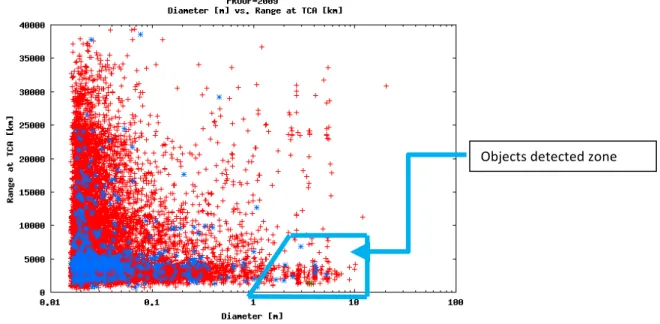
Figure III.1-3: Observation Scenario 1: debris detection performances

The simulations (Figure III.1-3) show that the system can detect medium-sized objects close to the satellite. It is possible to detect objects starting from 0.5m at a distance lower than 5000Km at the Time of Closest Approach (TCA) to objects of 5 meters at 25000Km.

III.2.

QB50-3Ucubesat

The second scenario investigates the possibility of using a star tracker suitable for a cubesat. This scenario aims to check the performance of a very low cost dedicated debris detector system, using a satellite with the dimensions of a cubesat and hardware already on the market, and modifying only the software. In this case the

(15)

15

cubesat needs to have a star tracker. Few star trackers are suitable to be used onboard a cubesat. One of them is the Blue Canyon Technologies (BCT) Nano Tracker (Figure III.2-1).

Figure III.2-1: BCT Nano Tracker(copyright Blue Canyon Technologies)

The dimensions of this star tracker are 100x67.3x50 mm including the baffle; nominal power consumption is less than 0.5W and the mass with the baffle is 0.35Kg. Its mechanical features make it suitable to be used on board a cubesat. This cubesat also needs an attitude control system, like the one developed by Gian Paolo Candini, with dimensions of less than 55x55x55mm (Figure III.2-2)

(16)

16

To take these components onboard, the volume of a 3U cubesat is required (Figure III.2-3).

Figure III.2-3: 3U cubesat main dimensions

The orbital parameters of the simulated observation system are: • Sun-synchronous polar orbit

• 98° inclination

• Nominal altitude of 700Km

The star tracker’s declared field of view is 9x12 degrees: simulating the star tracker point against the sun it is possible to simulate the detectable objects with the PROOF software.

Figure III.2-4: Observation Scenario 2: debris detection performances

(17)

17

The simulations (Figure III.2-4) show that only fragments which are bigger than 1m and have a range at TCA of about 5000Km can be detected.

III.3.

Satellite for general survey

This scenario evaluates the development of a generic satellite with hardware dedicated to space debris surveillance. With the data coming from the previous simulation, it is possible to see that the best solution is to have a telescope with a wide diameter and a short focal distance: but at the same time the mission has to be cheap. The weight and the dimensions have to be suitable for a microsatellite. To have a cheap mission it has been decided to not develop a completely new telescope, but to adapt a terrestrial telescope to work in the space environment (see Hardware chapter). Looking in the terrestrial telescope market, one of the best telescopes found with the required characteristics is the RILA400 model (Figure III.3-1), produced by an Italian company.

The telescope features are: • Type: Riccardi-Honders

• Primary mirror diameter: 400mm • Focal ratio: F/3.8

(18)

18

Figure III.3-1: RILA400 telescope(copyright Officina Stellare srl)

The orbital parameters are similar to the previous simulations: • Sun-synchronous polar orbit

• 98° inclination

• Nominal altitude 700Km

Figure III.3-2: observation scenario 3: debris detection performances

(19)

19

In this case, the objects detected start from 0.1m, one order of magnitude smaller than in the previous cases analyzed (Figure III.3-2).

III.4.

Satellite to survey Cosmo SkyMed

orbital plane

In this scenario the aim is to see the performances of a surveillance satellite dedicated to protecting the CosmoSkymed Italian constellation using the same hardware used in the third scenario. For this reason the orbital parameters are (Figure III.4-2):

• Sun-synchronous polar orbit

• Nominal altitude of 750Km (about 100Km above the CosmoSkymed altitude) • Telescope pointing tangent to the CosmoSkymed orbit

In this way it is possible to continuously check the CosmoSkymed orbit and maximize the results.

(20)

20

Figure III.4-1: Cosmo-Skymed survey satellities orbit

Figure III.4-2: observation scenario 4: debris detection performances

Objects detected zone

(21)

21

Compared to Scenario One, where the CosmoSkymed onboard star tracker is used, the dimensions of the objects detected are ten times smaller, and in this case objects up to a centimeter are detected and also the checked range is wider (Figure III.4-2).

III.5.

Conclusion

The simulation shows that it is possible to use the on board star mapper to check the space around the satellite. In this case, the objects detectable have medium size and are closer to the earth.

The development of a 3U cubesat satellite with the existing hardware is an option able to check only near and big objects.

The best solution maintaining low budget hardware is to develop a dedicated space surveillance microsatellite (less than 100Kg). In this case, it is possible to detect a very wide range of objects, up to a cm in diameter, and in this way to protect some particular orbits.

(22)

IV. Software

In optical observation systems, one of the main problems is the extraction of the right information concerning the debris from the pictures, in particular for the extraction of an accurate angular measurement. Usually, the telescope nominal pointing angles, namely right ascension and declination, and the time of acquisition are recorded in the picture, embedded in the image information according to well established standards. However, this angular information is adversely affected by the telescope mount mechanical pointing errors, with huge limitations in the achievable space debris measurement accuracy. A much more accurate angular information can be obtained by comparing the object light track with the background star field, against accurate star position available from astronomical catalogues ([12],[13],[14]) as described for example by Porfilio, Piergentili and Graziani [16] [17]; Santoni, Ravaglia, Piergentili, [18] and Schildknecht, Musci, Flury [19]. In addition, through light curve evolution in time, it is possible to obtain information about the rotational status of orbiting objects [20].

The extraction of this accurate information requires the identification of the star field in a typically large field of view (for surveillance campaigns), by finding the best superposition of the star image with the star catalogue. This process involves hundreds of stars per image, which must be compared to a previously unknown number of stars in the catalogue. This astrometric calculation, which is not just an image analysis process, but involves the analysis of tens of thousands of possible configurations to detect the correct field, is a time consuming and computation intensive process, which often requires the assistance of a human operator to solve particular cases.

(23)

Ch a p te r: IV S o ft w a re

23 IV.1.

Ground Software

IV.1.1. Image analysis software overview – ground

software

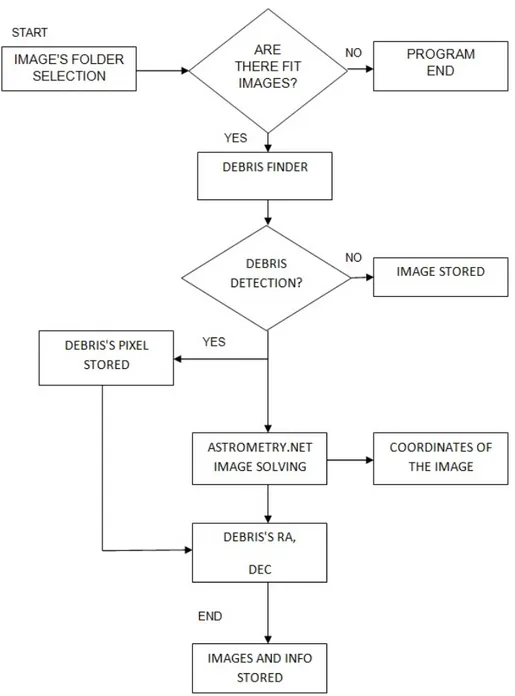
The algorithm stream of the image analysis, shown in Figure IV.1-1, is based on three main steps.

• The first step is where the software searches for astronomical images stored in a specified folder. At this stage a list of files has to be analyzed and then it is initiated and images are opened for the first time. The input images are in .fit file format. The preliminary operation on the images is the search for debris. A comparison between the images is not used and every image is used alone. If no object is detected within the image, it is stored in a spare folder. In the case in which there is a positive detection, the image goes ahead in the analysis process.

• The second step is the measurement of the image centre right ascension (RA) and declination (Dec) angles using information from the USNO-B catalogue. This step is based on the star identification using a “lost in space” case procedure, thus not using any information taken from the image file header; at least four stars are needed. Even if this procedure is time consuming, it permits us to apply the software to any astronomical images, even to images with a corrupted fit header. This step is based on some libraries taken from the open source software “astrometry.net” that allows us to obtain the RA and Dec

(24)

Jacopo Piattoni PhD thesis Ch a p te r : IV S o ft w a re

24

angles of the centre of the picture and its orientation with respect to J2000

Equator and Mean Equinox J2000.0 [21].

• The last step is the identification of the space debris RA and Dec angles. It consists in comparing the position of the debris centroid with respect to the image reference. The information stored and the end of the process are jpg images containing all the sources found (star and debris) and text files containing the position in the image and position in the sky of the found objects.

(25)

25

The image analysis software has been conceived as a standalone system working in a Linux environment; written in a large part in C programming language. The output of the complete process is stored in a new folder for each image with positive detection. In this folder there is all the information produced for the images: (i) space debris centroid RA and Dec angles, (ii) space debris centroid coordinates in image reference frame, (iii) image main evaluated characteristics (i.e. field of view, orientation, image center RA and Dec angles, pixscale…), (iv) stars identified during the mapping process as found from step 2 output, (v) space debris identification as found from step 1 output.

The software that implements the whole procedure has been made friendly user by developing a simple GUI (Graphical User Interface) that assists the operator in the software setup and launching phases.

IV.1.2. The detection procedure - ground software

The analyzed images can be very different from each other because they can be acquired with different hardware, different strategies and different environmental conditions. All these parameters influence the quality of the images, the background and the noise. Furthermore, the tracked shapes can have different geometrical properties from image to image.

The software can analyze pictures acquired with or without sidereal tracking. The differences in the acquiring strategies influence the information on the images. With the tracking, the stars are recorded as a Gaussian or Lorentzian function, while the debris has a streak shape. Without the tracking, orbital parameters affect debris/earth relative motion and accordingly also the images.

For the sake of generality, and aiming to make available the software to the larger experimenters’ community the debris detection software has been developed to work

(26)

26

both in the case of tracking on and off, taking into account the differences in the above described scenarios.

For a short exposure time all the sources (moving or not) are quasi-point-like but if the telescope is tracking in a Earth-fixed Reference System just the GEO objects are point-like sources while the stars and objects in other orbits leave trails. The exposure time and the pixel scale are a key point in the determination of the trails longitude both in sidereal tracking and when the telescope is fixed. The time exposure has been set as short as possible, in order to highlight the difference between pointlike and streaking objects without obtaining streaks so long as to decrease the accuracy of centroid determination and to risk superimposing streaking and pointlike objects. The time exposure was set to values ranging between 5 and 10 seconds obtained after a software calibration campaign; the GPS clock system is used as the external signal to trigger CCD shooting, thus leading to accuracy estimated through a dedicated calibration campaign, in the order of the microsecond.

If the tracking in enabled the problem is to detect the debris strips and the circular stars scattered over the background. Vice versa when tracking is off the detect strips are computed as stars and the circular detection as debris.

The image analysis procedure starts with a checking of the image integrity, which is carried out using a standard background analysis technique (e.g. checking if the characteristics of the images respect the information in the header); images corrupted due to bad saving/moving operations or which have been taken during telescope slewing are rejected.

The following operation is to detect star and debris tracks in the black space background: this is obtained by selecting a threshold (dependent for ex. by the instruments used for image collection, weather) and finally by saving the image as a black & white Bitmap. In this new image the pixel assumes the value 0 for black pixels and 1 for white pixels.

The software calculates the threshold for each image considering the information inside each image. The software divides the original image into different sub images. This is because different portions of the images can have different brightness, different background and star value. Each sub image is filtered independently with its own threshold calculated taking into account the max, min, mean and standard deviation of

(27)

27

the pixel value. There is also the possibility of deleting a single point (hot pixels or cosmic ray detections).

The threshold starting value was set after the calibration campaign. Moreover, a manual correction can be introduced changing the threshold evaluation process. In this manner, it is possible to make the software more or less sensitive depending on needs in taking into account also fainter objects or in reducing the number of false detections.

It is thus converted into a matrix with numbers of rows and columns equal to the number of pixels of the image, and values of 1 for stars, debris, cosmic rays, hot pixels and noise.

The algorithm should now join the neighboring pixels representing the same star or debris and later discriminate debris tracks from stars.

A methodology has been developed in a way to join pixels belonging to the same star or debris, and it is followed by a neighboring rule: if a pixel is close to another one or to a group, it is considered as a part of the same star or debris. The application of this method to crowded images requires setting a high threshold value to avoid blended stars, thus leading to a percentage of lost data in faint objects.

Attention has also been focused on the computational time, aiming to develop an algorithm as fast as possible.

Figure IV.1-2: Scanning procedure

The idea for detecting the star or debris inside the image is to scroll the images giving a number, Pjk, to each group of connected pixels. This happens in two steps. In the

first one the nearest pixels are tagged as members of the same object. For some irregular shapes this is not enough and a second step checks further if some groups of pixels tagged as different objects are in reality only one.

Figure IV.1-2 shows an example of the detection method: the image is scrolled in the first step row by row, starting from the top left-hand corner of the image (Figure IV.1-2a). The first pixel which has a value equal to 1 assumes the value 2, so that

(28)

28

pixel Pjk=β, where j is the index of lines, and k is the index of columns; β is equal to 2,

and afterwards it is increased by one, so that β=β+1 (β=3 in this example). The row scan goes on until a new pixel with Pij=1 is found; a search of the 8 (3 or 5 if corners or

external rows or columns) neighboring pixels is carried out. If one of the neighboring pixels presents a value larger than one (Pmn= γ with row m, column n, γ >1), it means

that the pixel is a part of an already labeled star or debris and the pixel assumes the same value γ, so that Pjk= γ (Figure IV.1-2 b and e). If none of the 8 neighboring pixels

presents a value Pmn >1, then the pixel represents a new star and it assumes the

value Pjk=β, and β is increased by one (β=β+1) (Figure IV.1-2 c and d).

While scrolling the image in this first step, each time a new star or debris is found, a new item in an objects list is added. Each item presents a series of tags like the number and row and columns index of the pixels which compose it. This list is updated during the scroll so that at the end the number of objects found in the image is known, as well as the number and position of pixels representing each one.

Figure IV.1-3: Scanning procedure, second scan step

But there is still the risk of errors in detecting tracks, since an irregular shape can be confused with two distinct objects, as Figure IV.1-3 shows: a second step is therefore necessary to put together these objects close to each other: the rows and columns index of the second object are added to the list which refers to the first objects, and the index of all other stars and debris are correspondingly changed.

In this second step, the objects are compared to each other, pixel by pixel, and if two neighboring pixels are detected the objects are glued together.

From a computational point of view, in the first run the algorithm performs an average number of comparisons equal to j*k+8*N, where j is the number of rows, k is the number of columns and N is the number of objects (stars and debris) detected. Cases of pixels on the edge of the matrix require fewer computations.

(29)

Ch a p te r: IV So ft w a re

29

The second scroll requires a mean number of comparisons of about (N-1)*(N-1)*kmean^2*η where kmean is the is the mean value of the pixels number of a object and

η a value =<1 is used for taking into account two factors: 1) the value of N during this comparison is not constant but decreases combining different objects in only one and 2) as soon as two objects are discovered to be part of one bigger object, the comparisons for the original objects are skipped.

Tests have shown that about 10% of the objects detected in the first step are merged with other objects in the second step.

The second task of the algorithm is to divide the objects into stars and debris. This operation is performed in a very simple but effective way by applying formula derived from the inertia theory of sections. As already mentioned, the object (star or debris) characteristics in terms of number of pixels and index of pixels representing it are stored in a list. With np the number of pixels of the p object, Xi and Yi (with i from 1 to

np) the width and height values in the images of the i pixel of the p object, it is possible

to calculate the centroid of the p object with the following Eq.1.

XCG and YCG are the coordinate values of the centroid of the p object. Once the CoG

has been detected for each object, the inertia axis Ixx about the x, Iyy about the y and

Ixy about the transverse axis can be computed with Eq.2.

Finally, the principal inertia moments (Imain1 and Imain2), can be found, together with the

orientation of the main axis respect to the horizontal reference of the image. (θ angle, positive defined if counter clockwise) with Eq. 3.

(30)

30

Finally, an object is defined as moving, and is labelled as possible debris if Eq. 4 is satisfied.

The definition of the ε parameter is a crucial task which is now accomplished manually, tuning its value after a series of trial and error tests. After a series of evaluations, the value of ε seems to be influenced mostly by camera features, speed of moving objects in the image and orbit of the object. Moreover, it changes with time because of the optical focus and because it could be different in the corners of wide FoV images due to aberration and collimation. A typical comparison between axis length in the case of a star (more or less equal) and in the case of moving debris (one axis far larger than the other one) can be found in Figure IV.1-4.

The value of ε used for the described campaign is 10; this means that if the streak is considered as a rectangle the longer side is three times longer than the short side.

Figure IV.1-4: Star and debris identification

IV.1.3. Stream of process – ground software

(31)

31

Figure IV.1-5: Test image

The elaboration starts transforming the picture from a grey scale image to a Black and White image (Figure IV.1-6a)

In this process the noise of the picture creates a sort of eliminated “dust” filtering the picture (Figure IV.1-6b), deleting isolated white pixel zones due to cosmic rays, hot pixels and the grey/BW conversion.

Upon this “cleaned” image the program starts to search, row by row, for the object in the picture. As described in section 3, after a first detection step (Figure IV.1-6c) some objects are detected as separated in different parts. In Figure IV.1-6ac it is shown how each object identified as a single one is highlighted in a different color. In this case the debris strip is wrongly identified as four different objects. A second detection step is required to deal with this situation in order to combine the parts in a unique object. The output of this step is shown in Figure IV.1-6d where it is possible to see that the debris strip is sketched in a single color standing for a single object tracklet. After this passage the software is able to separate the stars from the other objects and to calculate the centroid of the objects themselves. The position of the object in the

(32)

32

image reference frame is also recorded. The successive elaboration is performed on the original image by the software astrometry.net.

The astrometry.net software implements an algorithm able to identify the stars in the images on the basis of the image star patterns (Figure IV.1-6e), using the “solve-filed” routine.

These patterns are compared with a database of polygonal figures preloaded and chosen in order to have large dishomogeneity among different parts of the sky.

When a match is found (Figure IV.1-6f), using the information of the star field, the position of the object is calculated saved the Ra and Dec of the image center and its orientation.

(33)

33

(34)

34 IV.1.4. Observation campaign

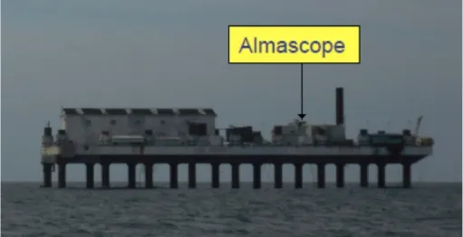
To verify the performance of the software we used data from a real observation campaign, carried out in the Italian Space Agency (ASI) Base in Malindi (Kenya) [22]. The observation was done using the ALMASCOPE observatory, based on a commercial off-the-shelf mount. The telescope used is a 25 cm f/4 in Newtonian configuration and the CCD is a Kaf1600E sensor, which has an array of 1024x1536 pixels, each pixel is a 9x9 micron (total chip size 9.2x13.8 mm) with shutter hardware controlled by GPS, in order to maintain epoch accuracy in the order of microseconds. The telescope field of view is of about 1 degree; the pixel scale is about 1.9 arcsec/pixel. The ALMASCOPE is shown in Figure IV.1-7.

Figure IV.1-7: ALMASCOPE observatory

Nine nights of observations were performed from the Broglio Space Center in September 2010, with the main aim of verifying the quality of measurements and evaluating the performance of an observatory at the base.

The observation campaign was carried out from two different sites: the first one inside the base camp and the second one from the SAN MARCO off-shore platform located 5 miles away from the coast (Figure IV.1-8). The observation strategies were with and without the tracking and the images were taken both for the GEO belt and the GPS-Glonass orbits.

(35)

35

Figure IV.1-8: Observatory on SAN MARCO platform

The light pollution was extremely low from the platform while inside the base camp it was present even if low. The visibility was extremely variable with the seasonal effect, it was estimated of about 4’’ in September that is in the wet season; the visibility improves during the dry season.

Further images come from a second observation campaign of four nights carried out in Rome, between 29th June and 2nd July 2013. In this case we used a 20 cm telescope f/4 in modified Cassegrain configuration and the CCD DTA1600 with an array of 1200*900 pixels; the pixel scale is about 3.5 arcsec/pixel. The images of this second campaign are focused on the GEO belt and a large part around the Hotbird 13A satellites; the images are taken with the sidereal tracking on.

IV.1.5. Results – ground software

To perform the test we used a dual Xeon X5560@2.80 GHz, 12 GB RAM and 300GB hard disk at 15,000rpm, operative system Ubuntu 9.04. The software was not optimized for a multi core processor and in order to obtain a faster result more instances of the program ran at the same time. In total 4,283 images were analyzed with a mean execution time of about 40 seconds per image including the stars and

(36)

Jacopo Piattoni PhD thesis Ch a p te r : IV So ft w a re

36

object RA/dec measurement calculation. The disk dimensions of the images are variable from about 750Kb to 3Mb “according to different binning” with a global dimension of 6.5Gb of data. No considerable differences were highlighted in software performances, due to different binning sets.

In Table I the results from the automatic analysis of the images are summed up.

Table I: summary results

The 4,283 images were all checked by visual inspection and 3360 objects were detected in 1552 images; the software correctly found 2940 objects in 1460 images. 2940 objects identified by the software out of 3360 objects identified with visual inspection on the same images leads to a success ratio of about 88% in the detection. For the sake of clarity, it should be noted that for testing purposes the images were collected in many different environmental conditions, even with bad natural light or artificial light pollution. Moreover, all the images used are in row format, subtracting the usual flat, dark and bias frames because, in this way, it is possible to increase the percentage of object detection successfully, reducing the false positive.

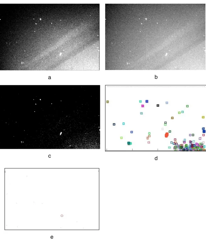
In Figure IV.1-9an examples of successfully analyzed images are shown to give an idea of the strip find system robustness.

(37)

37

a b c _d e

Figure IV.1-9: An example of bad images with noise and hot line: a) original image; b),c) image after different cleaning phases d) pixel selected to be analyzed; e) object detected

(38)

38

The most common detection error was made when two close stars were confused as a possible satellite strip. Other common error sources were due to stars cut by the border of the image and noted as possible satellites. This is due to the fact that the cut changes the shape of the star from a circular to an elongated shape. Another important source of mistakes is the hot lines in the images.

For each strip found the program wrote a txt file with the RA and Dec of the debris (Figure IV.1-10).

Figure IV.1-10: Image with the results

A group of 17 random strips were chosen to be calculated also with Astrometrica software (an interactive software tool for scientific grade astrometric data reduction of CCD images, http://www.astrometrica.at) in order to compare the results. (Figure IV.1-11).

(39)

39

Figure IV.1-11: RA and Dec difference between the new software calculation and the Astrometrica software result

Astrometrica software was used to extract the centroid of the short strips, thus calculating the measurements required for orbit determination. When strips were too long and the centroid could not be easily calculated directly by astrometrica, the positions of the initial and final strip pixels were measured and their central position was extracted through simple linear interpolation.

The RA standard deviation is 4.55 arcsec; the standard deviation is 1.57 arcsec.

The large distribution of standard deviation is mainly related to the manual procedure of astrometrica; nevertheless, the low mean value difference seems to confirm that the astrometrica procedure can be substituted by the developed software.

(40)

40 IV.2.

Space Software

IV.2.1. Image analysis software overview – space

software

Based on the experience done with previous software, new software has been written. The different requirement for this second software is the ability to work in a satellite platform and this basically means to work with a different hardware and computational resource compared to the first software. The most important innovations are:

• The software is totally written in C and external software is not used. The software can be compiled in a very wide range of hardware classes. The C program language guarantees high compatibility and fast computation time. • New object detection procedure. The detection procedure is completely revised

and based on the Canny edge multi-stage detection algorithm. • New space solve field engine

IV.2.2. The detection procedure – space software

The detection procedure uses the previously described way of recognizing the object shape, but compared to the previous software, it uses the images in a way that they are preprocessed in order to identify the edge of the objects (Figure IV.2-2). Once the

(41)

41

edges are obtained, the detection procedure is similar to the previous one. In order to identify the edge of the object, the Canny edge detector algorithm is used [23].

The edge detection is a ten-step process:

1) The first step is to recognize the pixel with relevant information in the image. For this purpose the image histogram has been calculated. Based on the histogram shape, two thresholds are determined. The pixels under the first threshold are considered black. This helps to eliminate part of the image noise. The pixels above the second threshold are considered white. In this way the hot spots are cut. A hot spot can generate false results, mismatched with a star, and requires useless computational time.

2) In the second step there is the convolution between the images with a Gaussian filter. This is essential to filter out the noise to protect the detection from mistakes caused by it. The result is a slightly blurred version of the original, clear of any speckles. The equation for a Gaussian filter kernel with the size of 2k+1x2x+1 is shown as follows:

Based on experience, the best results for this application are obtained using a 15x15 mask, with a sigma coefficient of 2.0. In this way each pixel is redefined as the sum of the pixel values in its 15x15 neighbourhood times the corresponding Gaussian weight, divided by the total weight of the whole mask. Calling A the pixel matrix and using the * to indicate the convolution operator, the pixel matrix B is:

where GKN is the normalised Gaussian mask.

3) The third step uses the gradient of the pixel to find the edge strength and direction. An edge may point in different directions and have different intensity.

(42)

42

It is possible to identify the intensity G and the direction θ using information from the first derivate in the horizontal direction (Gx) and vertical direction (Gy)..

For this calculation the Sobel masks are applied to the 3x3 pixel neighbourhood of the current pixel, in both the x and y directions.

Then the sum of each mask value times the corresponding pixel is computed as the Gx and Gy values, respectively. Calling B the pixel matrix at this stage and using the * to indicate the convolution operator, the matrix are:

4) The fourth step is the non-maximum suppression. This operation determines if the pixel is a better candidate for an edge than its neighbouring pixel. The result is a matrix where all the gradients are 0 except the local maximal, which indicates location with the sharpest change. In order to identify the edge correctly, first of all the pixel direction is checked. If this pixel is a local maximum, the gradients of the pixels in the perpendicular direction have to be lower than the pixel gradient itself.

First of all, the edge direction angle is rounded to one of four angles representing vertical, horizontal and the two diagonals. Then

• if the rounded gradient angle is zero degrees (vertical) the point will be considered to be on the edge if its gradient magnitude is greater than the magnitudes at pixels in the horizontal directions,

• if the rounded gradient angle is 90 degrees (horizontal) the point will be considered to be on the edge if its gradient magnitude is greater than the magnitudes at pixels in the vertical directions,

(43)

43

• if the rounded gradient angle is diagonal the point will be considered to be on the edge if its gradient magnitude is greater than the magnitudes at pixels in the opposite diagonal directions.

5) The fifth step is the hysteresis thresholding. Large intensity gradients are more likely to correspond to edges than small intensity gradients. Two thresholds are used: high and low. The high threshold identifies that the pixel is surely on an edge while the low one shows that the pixel is certainly no part of an edge: but for most of the pixels, the value of the gradient is between these two thresholds. Making the assumption that important edges should be along continuous curves and using the directional information derived earlier, edges can be traced through the image.

For each pixel candidate to be an edge pixel between the two thresholds the information of the neighbor’s pixels along the edge pixel direction is analyzed. If a pixel is indicated as part of a vertical edge but its gradient value isn’t higher than the high threshold, the pixel above and below are checked to verify if they are also part of a vertical edge. This is done for all the directions and in this way all the pixels are identified as part of an edge or not.

Figure IV.2-1 shows the result of the canny edge detection overlapped in fuchsia on the original images.

(44)

44

Figure IV.2-1: edge detection

6) The sixth step is similar to the one described in the “The detection procedure” chapter. The main difference is that it is now applied only to object edges and not to the whole object. For this reason the pixels analyzed are fewer and this step is faster than in the previous software. Sometimes the edge is not continuous as it can have a pixel missing, the algorithm capable to recognize objects even with two continuous pixels missing.

7) The seventh step is activated only if there is detection of objects different from stars. In that case the image is interesting and will be processed further in order to determine the position of the objects in the sky. In that case the detection routine also extracts the position of the star in the image.

Based on the image information extracted in step 1, two new thresholds are determined: the pixels under the first threshold are considered black and the pixels above the second threshold are considered white. The “black” threshold is higher than the one used in step 1. This means that the points considered as black are brighter than before. This is possible because the stars used for the star filed recognizing process are usually brighter than the satellites in the images. This helps to cut a lot of noise from the image and speed up the

(45)

45

elaboration. The “white” threshold is also higher than the one in step 1. The value of a pixel is related to how many photons are received by the CCD and a star with higher magnitude will create a zone with a higher number of photons. Step 1 is oriented to finding objects and not to calculating which object is the brightest. Considering a lower “white” threshold means all pixels above the threshold level are white and this causes a loss of information. However, in the first step that information is not relevant. Now in this step this information is relevant and allows us to identify the magnitude of the stars.

8) Once the new pixel values have been computed, the detection method used is similar to the one described in chapter IV.1.2 and a list of stars is created. The list is sorted by the magnitude value of the stars. The pseudo-magnitude is a value related to the brightness of the star, calculated using the pixel information. It isn’t the real magnitude because it is impossible to know the real star magnitude with only one image, without other information, but counting the pixel value is possible in order to create a classification of star magnitude in the image.

9) The position of the star is checked against the debris position. If the star is to close to the debris, is not considered. This is done to eliminate possible debris calculated as a star or a star too close to debris. Stars and debris which are too close can create false detection.

10) At the end of the process two files are recorded: one with the position in the image of the object and one with the position of the star with its pseudo-magnitude value.

(46)

46

(47)

47 IV.2.3. Space solve field engine

The new engine is based on triangle patter recognition. Starting from the detection of the star in the picture, triangles are hypothesized based on star brightness and position. The triangle is searched for in a previously prepared database. The database is built using the 2.5 million brightest stars taken from the star catalogue Tycho-2.

IV.2.3.1.

The star index

In order to recognise the triangle created using the stars in the images, a triangle database of the whole sky, or only a part of it, was previously prepared. This is based on the star catalogue Tycho-2. This is a catalogue of more than 2.5 million of the brightest stars, collected by the star mapper of the ESA Hipparcos satellite.

Different sets of indexes can be created. If the information about the FOV of the image is available, an ad-hoc index can be created for that FOV. If this information is not available, different sets of indexes, using different FOV, can be produced and used for pattern recognition. The second option creates indexes which are huge in comparison to the first option and the computational time to create and to search in the index increases. In case the index is very long, usually for images with very low FOV, it is better to split the index into parts representing different sky zones in order to obtain files with dimensions which are easier to load and read.

The index creator file steps are:

1. The index creator file starts reading the whole Tycho-2 catalogue.

2. Starting from a desired point in the sky, the software identifies the star in a box with area of about 1/6 of the image. This is because the position of the orientation and position of the image are random compared to the orientation of the box. Choosing a box size of about 1/6 of the image, surely at least one box is completely in the analysed image.

(48)

48

3. The stars in the box are listed and sorted by magnitude. The stars with lower magnitude have a higher probability of being recognised in an image. Depending how many images are found in the box, two different elaborations are carried out: 3.1. If there are three or more stars it is possible to create a triangle path between

the stars. In order to limit the index size, maximum two triangles per box are recorded. The triangles recorded are the ones created between the brightest stars in the box. For this reason, only the three brighter stars are used.

3.1.1. For each possible triangle the distances between the three stars composing the triangle are calculated.

3.1.2. Using the higher distance, the three distances are normalised. In this way two pieces of information are extracted: two relative distances of the stars that can be used as sides of the triangle.

3.1.3. The angle between the two previously extracted sides of the triangle is calculated.

3.1.4. Now all the information about a triangle can be written in the index, representing one row:

! Side one ! Side two

! Angle between the previous sides ! Ra of the brightest star of the triangle ! DEC of the brightest star of the triangle ! Ra of the medium bright star of the triangle ! DEC of the medium bright star of the triangle ! Ra of the dimmest star of the triangle

! DEC of the dimmest star of the triangle

3.2. If the stars are fewer than three, only information about their positions is recorded.

4. Once the analysis of one box is completed, the box is moved to another position in order to cover all the interesting zones of the sky.

(49)

49

(50)

50 IV.2.3.2.

The solver routine

Once objects have been detected by the detector routine, the star field solve routine is activated. This routine can be divided into three main parts:

! Creation of a list of triangles using the stars in the image

! Search in the already compiled star index for the extracted triangles and identification of the stars in the image

! Identification of the objects’ Ra and DEC

IV.2.3.2.1.

Triangle identification

The number of figures with k sides that it is possible to calculate starting from n point is calculable with combinatory math.

For any set containing n elements, the number of distinct k element subsets of it that can be formed is given by .

Using the factorial function, can be written easily as:

In this case, k always equals 3 and n is the number of stars. The maximum possible triangles are (Table II):

• Stars • Triangles • n=4 • 4

• n=5 • 10

• n=6 • 20

(51)

51

• n=8 • 56 • n=9 • 84 • n=10 • 120 • … • … • n=15 • 455

Table II: Star numbers and possible triangle combinations

The number of triangles rises very fast. This is the maximum number of triangles that can be created. But not all these triangles are suitable for the star field identification.

As already shown in the index creation, the useful triangles cannot be bigger than 1/6 of the images, otherwise they are not in the index. Furthermore, only the brightest stars are used for the triangles in the index. This means that only a small part of the theoretical triangles are potentially in the index. The star distribution and magnitude cannot be previously determined and this means that it cannot be determined theoretically how many useful triangles there are in the image.

After tests, it was decided to extract as many triangles as there are stars in the images. The triangle sides have to be smaller than the 1/6 of the images and have to be created with the brightest stars in the images.

Once these parameters are fixed, the algorithm can start:

1. The star position in the image and the pseudo-magnitude are read. 2. The stars are sorted by pseudo magnitude.

3. The brightest star is taken as the first vertex of the triangle. 4. The second brightest star is taken as the second vertex.

5. The distance between the two stars is checked. If it is higher than 1/6 of the image dimensions, the second star is changed with the next star until stars with distances within the limit are found.

6. Once the first two stars have been fixed, the last star is searched for among the remaining stars, always starting from the brightest and looking to see whether the distances from the other two stars are within the limit.

7. Once one triangle has been identified, the algorithm repeats the process from point 4 to point 6. If there are no more suitable combinations using the brightest star as

(52)

52

first vertex, the second brightest star becomes the new first vertex and so on. Every time a new potential triangle is found, it is necessary to check whether it has already been identified, using the same stars but in a different order.

8. When the decided triangle number has been identified, the triangle is transformed into information that is compatible with the index. The sides are calculated and normalized using the longer side and the angle between the two non-maximum sides is calculated.

9. Information about the triangle is recorded in a table in the same order as in the index:

! Side one ! Side two

! Angle between the previous sides

! X-pixel of the brightest star of the triangle ! Y-pixel of the brightest star of the triangle ! X-pixel of the medium bright star of the triangle ! Y-pixel of the medium bright star of the triangle ! X-pixel of the dimmest star of the triangle ! Y-pixel of the dimmest star of the triangle

(53)

53

(54)

54 IV.2.3.2.2.

The triangle choice

Once the triangle candidates have been identified, the triangles have to be searched for in the index. The research is carried out in two stages.

In the first one every triangle is searched for in the index. A ranking is created with the most probable triangles and one by one the solutions are analyzed: but this isn’t enough because among the hundreds of thousands of index triangles, a lot of them are very similar. It is clear that using only the three pieces of information about two sides and one angle is not enough to identify a triangle that is similar in the index and in the image.

In the second stage for each possible solution the ability to predict the position of the other stars in the picture is evaluated. In this way, not only the information about the three stars used as triangle vertices is used, but also the information about the other stars in the images. Depending on the picture field of view, if a solution is able to predict the position of the other stars with a certain maximum allowable error, it is considered a valid solution.

1. The routine starts by opening the index file, reading and loading the whole index content.

2. The triangles are searched for in the index. The search is carried out on the three triangle parameter, considering a possible error. In fact, the triangles extracted from the catalogue and the ones extracted from the image can be slightly different for noise, image deformation and pixel discretization. Two parameters are set: the acceptable percentage error in the dimensionless sides and an error in degree in the angle. If these parameters are too high, the execution time increases rapidly. On the other hand, if they are too low some significant triangles can be discarded. From the test, an error value of 1% in the side dimensions and 1° in the angle is an acceptable value.

(55)

55

3. If a triangle in the index has all the requested features to be similar to a triangle in the images, the difference between the two triangles is calculated. Taking into account the difference in sides and angle, a value of similarity is computed. At this stage, from the hundreds of thousands of index triangles, about a thousand are selected.

4. At this stage the possible solutions are geometrically transformed one by one. The triangles in the index and in the image are similar but have different dimensions, orientation and position. In order to overlap the two similar triangles, the triangles in the image are transformed and the information about the brightness of the triangle’s stars is used.

4.1. The first transformation is the rotation. The lines between the two brighter stars in the index triangle and in the image triangle are calculated and the angle between the two lines is extracted. The image triangle is rotated by this angle.

4.2. The second transformation is the scale. Taking into account the side length between the two brighter stars in the two triangles, a scale factor is applied to the image triangle.

4.3. The third transformation is the translation. The distance between the brightest stars in the two triangles is calculated and the image triangle is translated to overlap the index triangle. In this way the brighter stars in the two triangles are overlapped.

4.4. In the last step the position of the dimmest star in the two triangles is evaluated. In this way also the information about the last star of the triangle is used and the capability of the solution found to predict the last triangle vertex position is evaluated. At this stage, in fact, all the information to calculate the Ra and DEC of every pixel in the image is available and is tested to calculate the Ra and DEC of the last image triangle star. If the solution is correct, the last star position will be foreseen within a certain range and the solution can continue in the next stages. The solution can make a wrong last star prediction for three possible reasons. The first one is in the rotation transformation. To calculate only the rotation angle is not enough to make a correct rotation; the rotation direction is also important. The second motivation is the image flipping.