Velocity-gradient statistics along particle trajectories in turbulent flows: The refined similarity
hypothesis in the Lagrangian frame
Roberto Benzi,1Luca Biferale,1Enrico Calzavarini,2,
*
Detlef Lohse,3and Federico Toschi41
International Collaboration for Turbulence Research and Department of Physics and INFN, University of Tor Vergata, Via della Ricerca Scientifica 1, 00133 Rome, Italy
2
International Collaboration for Turbulence Research and Laboratoire de Physique, École Normale Supérieure de Lyon, CNRS UMR 5672, 46 Allée d’Italie, 69007 Lyon, France
3International Collaboration for Turbulence Research and Department of Science and Technology, Impact Institute,
and Burgers Center, University of Twente, 7500 AE Enschede, The Netherlands
4
International Collaboration for Turbulence Research and Department of Physics and Department of Mathematics & Computer Science, Eindhoven University of Technology, P.O. Box 513, 5600 MB Eindhoven, The Netherlands
共Received 29 June 2008; revised manuscript received 20 November 2009; published 29 December 2009兲
We present an investigation of the statistics of velocity gradient related quantities, in particular energy dissipation rate and enstrophy, along the trajectories of fluid tracers and of heavy/light particles advected by a
homogeneous and isotropic turbulent flow. The refined similarity hypothesis共RSH兲 proposed by Kolmogorov
and Oboukhov in 1962 is rephrased in the Lagrangian context and then tested along the particle trajectories.
The study is performed on state-of-the-art numerical data resulting from numerical simulations up to Re
⬃400 with 20483collocation points. When particles have small inertia, we show that the Lagrangian
formu-lation of the RSH is well verified for time lags larger than the typical response time p of the particle. In
contrast, in the large inertia limit when the particle response time approaches the integral time scale of the flow, particles behave nearly ballistic, and the Eulerian formulation of RSH holds in the inertial range.
DOI:10.1103/PhysRevE.80.066318 PACS number共s兲: 47.27.⫺i, 47.10.⫺g
I. INTRODUCTION
One of the most prominent features of turbulent flows is the strong variation present in the energy dissipation field, a phenomenon called intermittency 关1兴. In an attempt to de-scribe quantitatively intermittent fluctuations in the inertial range of turbulence, Kolmogorov and Oboukhov in 1962 关2,3兴 proposed a general relation linking velocity fluctua-tions, measured at a given spatial increment ␦ru = u共x+r,t兲 − u共x,t兲, with the statistical properties of the coarse grained energy dissipation, r= r−3兰⌳共r兲共x,t兲d3x averaged over a volume,⌳共r兲, of typical linear size r,
␦ru⬃ r1/3r1/3, 共1兲 where⬃ means “scales as” or “equal in law.” Equation 共1兲 is known as the refined 共Kolmogorov兲 similarity hypothesis 共RSH兲 and it is considered to be one of the most remarkable relations between turbulent velocity fluctuations: Many ef-forts in the last decades have been devoted to its validation 关4–6兴. The importance of RSH cannot be underestimated: it bridges inertial-range properties with small-scale properties, supporting the existence of an energy cascade mechanism, statistically local in space. So far, a rather strong evidence supports the validity of the RSH in the Eulerian frame共i.e., the laboratory frame兲. On the other hand, no investigation has been reported in the literature on the validity of RSH in the Lagrangian frame 共i.e., along fluid particle trajectories兲. The main difficulty in studying RSH in a moving reference frame stems from the necessity to make multipoint measure-ments along particle trajectories in order to calculate the
stress tensor. As a result, no experimental measurements along particle trajectories of velocity gradients exists for time long enough to be able to evaluate temporal correla-tions. Also numerical experiments are very demanding, re-quiring refined computations of velocity differences along particle trajectories. This is usually implemented by comput-ing the velocity gradients matrix in Fourier space, then trans-forming it to physical space by 共inverse兲 fast Fourier trans-form, and performing off-grid interpolations of the gradients at the particle positions. Here, we report the first of such measurements using high-resolution direct numerical simula-tion 共DNS兲 investigations. We also note that when the par-ticles transported in a turbulent environment have non-negligible size or mass, i.e., they are inertial particles, their trajectories becomes strongly sensitive to the statistical and topological properties of the advecting flow关7–10兴. The pos-sible validity of Lagrangian RSH in this context is far from being trivial and may shed new light on the physics of par-ticulate transport in turbulent flows: an ubiquitous phenom-ena in nature and in industrial applications alike.
In the present study, we will extend the RSH relation to the temporal domain and test its validity along the trajecto-ries of fluid tracers and of inertial particles whose density is smaller/larger than the fluid one while their sizes span the interval from the dissipative to the inertial range of scales. The paper is organized as follows. First we give details on the numerical methods of the DNS. We then present the ex-tension of RSH to the Lagrangian domain and we test it on the trajectories of fluid tracers. In the last section we inves-tigate the case of inertial particles: we show under which conditions the Lagrangian RSH still holds and how it should be modified in the special case of highly inertial particles. *[email protected]
II. NUMERICAL METHODS
The incompressible fluid velocity, u共x,t兲, ·u=0, evolves according to the Navier-Stokes equations,
Du Dt ⬅ u t + u ·u = − p f +⌬u + f, 共2兲 where p denotes the pressure,fis the fluid density assumed constant, and f is an external large-scale forcing injecting energy at a mean rate具典=具u·f典. Together with the Eulerian field we integrated the Lagrangian evolution of fluid tracers:
dx共t兲/dt=v⬅u关x共t兲,t兴, and point particles by means of a
model of dilute suspensions of small passively advected spherical particles, as derived in 关11–13兴,
dx dt =v, dv dt = Du Dt + 1 p 共u − v兲, 共3兲
where x andv denote the particle position and velocity,
re-spectively. In Eq.共3兲, the coefficient= 3f/共f+ 2p兲 is re-lated to the ratio between the density of the particle共p兲 and of the fluid共f兲;p= a2/共3兲 is the particle response time, with a as the particle radius. The Stokes number of the par-ticle is defined as St=p/, where ⬅共/具典兲−1/2 is the dissipative time scale of the turbulent flow. In our simulation the parameters and St can be varied independently, there-fore, it is possible to consider also the case共= 0 , St⬎0兲, corresponding to the limit to very heavy particles for which the fluid added mass is negligible while Stokes drag is the only relevant dynamical force. On the other hand the situa-tion共= 1 , St= 0兲 is equivalent to the case of a perfect fluid tracer.
Equation共2兲 is numerically integrated by means of a stan-dard internally 2/3 dealiased pseudospectral algorithm with a second order Adams-Bashforth time-advancing scheme. The very same time scheme is used to track the particles evolving according to Eq. 共3兲: the time-step size in both cases is
O共10−2
兲, however, particle informations are recorded for
postprocessing/analysis at a rate of 10−1
. Interpolations of
the velocity field, acceleration field 关necessary for Eq. 共3兲兴 and velocity gradients at the particle positions, are done via a trilinear algorithm. For a validation of our numerical method we address关14,15兴, where a satisfactory comparison on ac-celeration Lagrangian statistics has been performed against an independent numerical implementation with several dif-ferent features共field interpolation based on tricubic scheme, external dealiasing procedure, a slightly different large-scale forcing兲. In our DNS energy is injected at large scale by maintaining the spectral content of the first two shells in Fourier space constant. Here, we will report data coming from two sets of simulations with N3= 20483 and N3= 5123 collocation points, corresponding to Re= 400 and 180, re-spectively, and sampling the parameter space 苸关0:3兴, St 苸关0:4兴 with 64共, St兲 particles types. A total amount of ⬃108particles are tracked in time. Results on the clustering of these particles in the turbulence have already been re-ported in 关8,9兴. Inertia requires some time before particles reach their fractal共or multifractal兲 statistically stationary dis-tributions 关16,17兴. We therefore waited till the Lagrangian statistics became stationary 共approximately one large-eddy
turnover time兲 before performing the analysis presented here. Measurements of velocity differences and gradients are based on sets of O共106– 107兲 particles which have been fol-lowed in time for few O共1兲 large-eddy turnover times.
III. REFINED SIMILARITY HYPOTHESIS IN THE LAGRANGIAN FRAME
A. Inertia effect on the statistics of principal invariants of velocity gradient tensor
We have already noted that the effects of inertia may be of particular interest for the present study. Inertial particles are not distributed homogeneously in the volume, centrifugal force tends to concentrate light particle inside strong ellipti-cal regions, with high vorticity关7,8,18兴, and heavy particle in hyperbolic regions, typical of intense shear. Following Chong et al. 关19兴, the flow topology may be locally defined in terms of the two principal invariants of the velocity gra-dient tensor A=Aij=iuj, namely, Q = −Tr关A2兴/2 and
R = −Tr关A3兴/3 共see also 关20兴 for a recent study兲. Q represents the difference between a rotation dominated and a dissipation-dominated flow topology, e.g., it is positive in a vortex core, while negative in a region characterized by high strain. The second parameter, R, analogously represents the competition between the vorticity production and the dissipation production. Also, the separatrix curve 共R/2兲2+共Q/3兲3= 0共so called Vieillefosse line 关21兴兲 discrimi-nate between three real or one real and two complex-conjugate eigenvalues for A, again meaning only strain or vortical regions. In Fig. 1, we show the joint probability density functionP共Q,R兲 for different particle types as mea-sured in the simulations at Re= 180. The most striking effect is for light particles 共= 3兲, contrary to tracers and heavy particles 共= 0兲 they spend essentially all of their time in upper half-plane Q⬎0, meaning that they constantly trapped in vortical regions.
B. Time correlation of symmetric and antisymmetric component of velocity-gradient tensor
One also expects pretty different temporal correlations be-tween particle trajectories and the underlying topology of the
tracer -8 -6 -4 -2 0 2 4 6 8 R* -8 -6 -4 -2 0 2 4 6 8 Q * β=0, St=0.5 -8 -6 -4 -2 0 2 4 6 8 R* -8 -6 -4 -2 0 2 4 6 8 β=3, St=0.5 -8 -6 -4 -2 0 2 4 6 8 R* -8 -6 -4 -2 0 2 4 6 8
FIG. 1. 共Color online兲 Joint probability density function
P共Qⴱ, Rⴱ兲 of Qⴱ⬅Q/具Q2典1/2and Rⴱ⬅R/具Q2典3/4for particles of dif-ferent types. Contour lines are drawn at values 10−zwith z = 0, 1, 2, 3, 4, 5, and 6共from the center to the outside of the figure兲. The thick line traces the curve:共R/2兲2+共Q/3兲3= 0共Viellefosse line兲,
discrimi-nating between complex共above兲 and real 共below兲 eigenvalues of A.
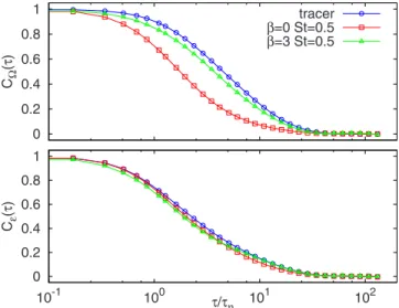
carrier flow. We look now at the symmetric/antisymmetric component of the velocity-gradient tensor A, because of their direct link with energy dissipation and enstrophy 关22–24兴. We show in Fig. 2 the autocorrelation function of enstrophy, ⍀=2共A−AT兲2=2兺i,j共iuj−jui兲2 and energy dis-sipation, ⑀=2共A+AT兲2=
2兺i,j共iuj+jui兲2, along the particle trajectories for different values of inertia. As one can see both these quantities have short autocorrelation time, at Re= 180 we find T⍀=兰0⬁C⍀共兲d⯝7 and similarly T ⯝5. However, the autocorrelation of enstrophy turns out to
be rather sensitive to the type of particles, while energy dis-sipation is probed more or less uniformly. This is a clear indication that due to inertia, particle tends to leave in re-gions with very different vorticity contents, while energy dissipation—although different in intensity—turns out to be a more robust quantity in term of coherence in time: This result will be very useful in our following discussion.
C. RSH and its generalized formulation
Along the trajectory of a fluid tracer x共t兲 the velocity difference will be denoted as␦v = v共t+兲−v共t兲 and similarly
we define a coarse grained energy dissipation measured along the trajectory as=兰tt+关x共t兲,t兴dt 共see also 关25兴兲. The RSH Eq. 共1兲 can be translated from space to time by making the assumptions that ␦v⬃␦ru and ⬃r when and r are linked trough the eddy turnover time definition, 共r兲⬃r/␦ru. This argument leads to the Lagrangian refined similarity hypothesis 共LRSH兲,
␦v⬃1/21/2. 共4兲 In order to test Eq.共4兲 one should verify, for any exponent p, the scaling relations,
具共␦v兲p典 ⯝p/2具p/2典, 共5兲 where ⯝ means equal apart from a multiplicative constant depending only on p, in the inertial range. In the time do-main the inertial range is defined as the interval, ⰆⰆTL, where TL is the Lagrangian integral time scale, which is estimated as the autocorrelation time of velocity of fluid tracers, i.e., TL=兰0⬁Cv共兲d, with
Cv共兲⬅具v共t兲v共t+兲典/具v2典. As one can estimate TL/⬃Re, the extension of the inertial range in dissipative time-scale units extends over roughly two decades in the present nu-merical study.
In contrast to the 4/5 law 共consequence of the Karman-Howarth equation兲 leading to exact scaling properties for third-order velocity increments in the Eulerian frame, we do not have any exact scaling relation derivable from NS equa-tions in the Lagrangian domain. Furthermore, it is known that in the Lagrangian frame, finite Reynolds effects induce larger deviations from a power law regime than what ob-served in Eulerian frame 关26兴. To overcome these effects, following 关27兴, we can generalize the above expression 共5兲 by using its extended self similarity 共ESS兲 form, namely,
具共␦v兲p典 ⯝
冉
具共␦v兲 2典 具典冊
p/2 具p/2典. 共6兲 D. Numerical tests of LRSHIn Fig. 3共a兲 we present a test of Eq. 共5兲 for p=4 for particles with= 1, St= 0, i.e., fluid tracers共circles兲 and very heavy particles with= 0, St= 2共triangles兲. In Fig.3共b兲, we show instead the relation from Eq. 共6兲 for the same particle types. Two major results emerge. First the LRSH, as ex-pressed by Eq. 共6兲 is well verified for the transport of par-ticles in turbulent flows. The use of the ESS version for LRSH is able to overcome finite size/time effects which are usually observed at relatively low Reynolds number 共see 关26兴兲. The second important result, which will be investi-gated later on in this manuscript, comes from inspecting the validity of Eq.共6兲 for different Stokes numbers. Equation 共6兲
0 0.2 0.4 0.6 0.8 1 CΩ (τ ) tracer β=0 St=0.5 β=3 St=0.5 0 0.2 0.4 0.6 0.8 1 10-1 100 101 102 Cε (τ ) τ/τη
FIG. 2. 共Color online兲 Temporal autocorrelation function, i.e.,
CX共兲⬅具X⬘共t兲−X⬘共t+兲典/具X⬘2典 with X⬘共t兲=X共t兲−具X典, of the
enstro-phy X =⍀ 共top兲 and the energy-dissipation-rate X= 共bottom兲 for
fluid tracers and for inertial particles with St= 0.5, =0,3, at
Re= 180. 10-810-610-410-2 100 102 <(δτv)2>2<ετ2>/<ετ>2 (b) 10-8 10-6 10-4 10-2 100 102 10-810-610-410-2 100 102 <( δτ v) 4> τ2 <ετ2>/<ετ>2 (a)
FIG. 3. 共Color online兲 Test of LRSH along the trajectories of
tracers and heavy particles at Re= 400.共a兲 For p=4 we show Eq.
共5兲 for St=0 共circles兲 and St=2 共squares兲. 共b兲 We show the validity
of Eq.共6兲 for the same values of p and St. Straight lines correspond
to the theoretical scaling prediction. Data come from Re= 400
is supposed to be valid both in the inertial range and in the dissipative range共where the velocity field is smooth兲 though with different offset. This is clearly observed in Fig.3共b兲for the case St= 0. It is already known that by increasing the Stokes number, particles tends to escape from strong vortic-ity region, thus decreasing the effect of the dip present in between dissipative and inertial scales 关28兴. As a conse-quence, for St= 2 we observe almost no deviation of Eq.共6兲 in the range of scales between the inertial and the dissipative ranges.
To have a more quantitative check, we look now at the ratio between the two sides of Eq. 共6兲, namely, at 具共␦v兲p典 divided by具p/2典具共␦v兲2典p/2具
典−p/2, as a function of the time difference . In Fig. 4, we show its behavior for the order
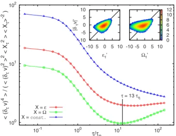
p = 4 fluid tracers particles, the time difference is normal-ized by the dissipative time scale . We observe a plateau 共see circles symbols, in Fig.4兲 for/ⱖ5. Notice that also in the dissipative range the compensation works well, as it should from the requirement that the velocity field becomes differentiable, ␦v⬃. However, the plotted ratio shows a mismatch with the value attained in the inertial range. The transition between the two plateaux occurs around the dissi-pative time scale, where the presence of vortex trapping has been shown to spoil the scaling behavior of Lagrangian structure functions 具共␦v兲p典 of the tracers 关29–32兴. In the same figure we show that using the coarse grained enstrophy, i.e., ⍀ instead of, the compensation is worse 共squares兲. Similarly, compensation with enstrophy does not work nei-ther for heavy nor for light particles 共not shown兲. Compen-sating without coarse grained quantities, i.e., checking the deviation from dimensional, nonintermittent, scaling does not provide a good plateau 共triangles in Fig.4兲. This result supports the validity of LRSH only when using the energy dissipation as the main driving process along the particle motion. The behavior for intense fluctuations 共moments
higher then p = 6兲 cannot be checked quantitatively due to the lack of statistics. Nevertheless, in the same figure, we show the joint probability density functions, P共⍀,兩␦v兩兲 and P共⑀,兩␦v兩兲, for a time lag = 13. Velocity increments are
more correlated with coarse-grained energy than with enstro-phy, as shown by the high probability measured for simulta-neous intense values of 兩␦v兩 and . Having established the validity of the LRSH, we strive now at investigating the effect of different Stokes number and different density prop-erties.
IV. LRSH IN THE (,St) PARTICLE PARAMETER SPACE
A. Heavy particles (=0) at StÈO(1)
When particles have inertia their trajectories deviate from material lines of the flow. In principle, one expects that for very small value of the inertia 共particles very close to fluid tracers兲 no appreciable discrepancies can be measured. In Fig. 5 it is shown the test for the LRSH compensated with the energy dissipation rate. From One can appreciate that in the inertial range, e.g.,/ⱖ5 the LRSH is well verified for all the Stokes considered. In the dissipative range it is also verified but with a different proportionality constant. In par-ticular, the important mismatch observed between the two plateaux for tracers in 共Fig.4兲 here is reduced considerable as soon as some inertia is switched on. This confirms that heavy particles are quickly expelled out of vortex filaments, and therefore much less sensitive to the transition around /⬃1 than tracers 关28兴 共the opposite will happen for light
particles, see below兲.
The behavior of the ratio 共AD/AI兲 of the plateaus dis-played by 具共␦v兲4典具
典2/共具2典具共␦v兲2典2兲 respectively in the dissipative range共ADforⰆ兲 and in the inertial range 共AI forⱕ10兲, is shown in the inset of Fig.5. The estimate for the slope of AD/AI vs St can be provided by the following 100 101 102 10-1 100 101 102 <( δτ v) 4 >/(<( δτ v) 2 > 2 <X τ 2 ><X τ > -2 ) τ/τη τ = 13 τη X =ε X =Ω X =const. -10 5 0 5 10 ετ’ -10 -5 0 5 10 |δτ v|’ -10 -5 0 5 10 Ωτ’ 0 2 4 6 8 10 12
FIG. 4. 共Color online兲 Test of LRSH along the trajectories of
tracers 共Re= 400兲. It is plotted 具共␦v兲4典/共具共␦v兲2典2具X
2典具X
典−2兲: 共circles兲 represent the case X=, 共squares兲 the case X=⍀, and 共tri-angles兲 the case X=const. In the inset the joint pdf: P共⑀⬘,兩␦v兩⬘兲 and P共⍀⬘,兩␦v兩⬘兲 at=13;共note that the prime symbol denotes vari-ables normalized respect to their mean values, i.e., x⬘⬅x/具x典兲.
100 101 10-1 100 101 102 <( δτ v) 4>/(<( δτ v) 2> 2< ετ 2>< ετ > -2 ) τ/τη heavy particles:β=0 tracer St=0.6 St=1 St=2 St=10 10 -1 100 101 10-1 100 101 102 AD /A I St
FIG. 5. 共Color online兲 Same as in Fig.4, here also along the
trajectories of heavy particles 共Re= 400兲. It is plotted
具共␦v兲4典具
典2/共具2典具共␦v兲2典2兲. Particles with St=0.6, 1, 2, and 10 are compared with the result for tracers共solid black line兲. The LRSH is satisfied both in the inertial and in the dissipative ranges. The pref-actors, AI and AD, however differs in the two regions. Notice that for the largest Stokes, St= 10, the smallest time lags where LRSH is verified, as expected, roughly⬃10. In the inset, the behavior of ratio of prefactors AD/AI is plotted vs St. For small St values a
reasoning. First we notice that the inertial constant AI is al-most insensitive from the Stokes value, therefore, the dissi-pative constant ADcarries all the St dependency. Moreover, we have measured that the single point energy dissipation statistics is pretty insensitive to the Stokes number共see again Fig.2兲. As a consequence the main dependency on St for the ratio AD/AI comes from the flatness factor F共兲 ⬅具共␦v兲4典/具共␦v兲2典2in the intermediate-dissipativelimit. It is reasonable to estimate the difference between F共兲 at changing Stokes, but fixed Reynolds, as given by the value of the flatness at the particle response time: F共p兲⬃St4−22, where p is the pth order scaling exponent for Lagrangian structure functions具共␦v兲4典⬃p. Based on the experimental values 4⯝1.6 and 2⯝1 关31兴, this estimate gives
AD/AI⬃St−0.4, not too far from the fit St−0.38⫾0.05to our nu-merical data, see inset of Fig.5.
B. Finite density contrast: Heavy and light particles
We now look at the statistical properties of particles with finite density contrast, i.e., also⫽0. In Fig.6it is shown, for St= 1, the behavior of the compensated tests for LRSH for different values ofspanning the full range关0:3兴. In the inset it is also shown the behavior, this time as function of, of the AD/AI ratio. Notice how the critical value = 1, dis-criminating between heavy共⬍1兲 and light 共⬎1兲 particles plays a crucial role. Again, LRSH is well verified in the inertial range, but the change to a different plateau around /⬃1 is now much more abrupt when light particles are
considered: for those the vortex trapping is more pro-nounced, as all light particles quickly move toward high vor-ticity regions, showing a very sensitive dependency around the dissipative time dynamics. A model for the dependency of AD/AI vs is presently not available.
C. Heavy particles (=0) with large inertia
Having studied the case of particles with small inertia, we now focus on the case of extreme inertia, i.e., when the
re-sponse time of the particle is at the top end of the inertial time range, or St⬃O共10兲. In this condition, for time lags ⬍p when the particle filters out most of the underlying turbulent fluid fluctuations and evolves nearly ballistically, one can predict a different behavior for ␦v. Along the
tra-jectory of a ballistic particle, the relation linking scale to time is 共r兲⯝r/v0 where the typical particle velocityv0 is proportional to root mean square fluid velocity. Recasting Eq. 共1兲 from space to time notation we obtain again an Eulerian-like RSH relation,共␦v兲⬃共/v0兲1/31/3, or
具共␦v兲p典 ⯝
冉
v0
冊
p/3
具p/3典. 共7兲
The generalized version of Eq.共7兲 reads now 具共␦v兲p典 ⯝ 具
p/3典
具⑀典p/3具共␦v兲 3典p/3
. 共8兲
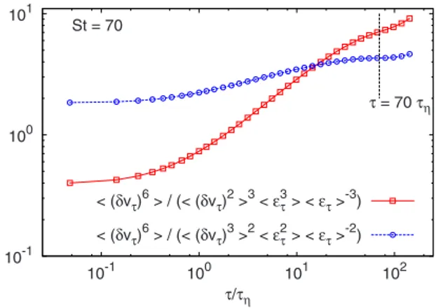
In Fig. 7, we present a test of this idea for 具共␦v兲p典 with
p = 6. For particles with very large Stokes numbers共St=70兲
we compensate the velocity increments both with respect to the prediction of the Lagrangian RSH and with respect to the prediction of the Eulerian RSH in its generalized version. The compensation with the Eulerian RSH works appreciably better in the range ⱕSt· than the compensation with LRSH.
V. CONCLUSIONS
In summary, some important statistical properties of ve-locity gradients along trajectories of fluid tracers, heavy and light particles have been investigated. We used high reso-lution high-statistic numerical data to correlate the temporal properties of velocity gradients and velocity differences along trajectories. We demonstrated that the refined similar-ity hypothesis is well verified both for fluid particles and particles with response time in the dissipative regime, a fea-ture that we dubbed Lagrangian RSH. Around the dissipative time lags, heavy and light particles behave strongly
differ-100 101 10-1 100 101 102 <( δτ v) 4 >/(<( δτ v) 2 > 2 < ετ 2 >< ετ > -2 ) τ/τη β=0 β=.5 β=.75 β=1 β=1.5 β=3 fixed Stokes: St=1 0 2 4 6 8 10 0 1 2 3 AD /A I β
FIG. 6.共Color online兲 Same as in Fig.4along the trajectories of heavy/light inertial particles with St= 1.0 共Re= 180兲. It is plotted 具共␦v兲4典具
典2/共具2典具共␦v兲2典2兲. Particles with=0, 0.5, 0.75, 1.0, 1.5, and 3.0 are compared with the result for tracers共solid black line兲. The LRSH is satisfied both in the inertial and in the dissipative ranges. As for the case of heavy particles the prefactors differs in the two regions. In the inset, the behavior of ratio of prefactors
AD/AIis plotted vs. 10-1 100 101 10-1 100 101 102 τ/τη St = 70 τ = 70 τη < (δvτ)6> / (< (δvτ)2>3<ετ3> <ετ>-3) < (δvτ)6> / (< (δvτ)3>2<ετ2> <ετ>-2)
FIG. 7. 共Color online兲 Particles with very large inertia do not
verify the LRSH共6兲 but follow the Eulerian version 共7兲. We show
this for the order p = 6 on particle trajectories with St= 70, at Re= 400. As it can be seen, in the inertial range, the Eulerian RSH compensate better than LRSH.
ently due to the effect of being expelled/concentrated out/in vortex filaments. The dynamics at those time lags becomes markedly dependent on the underlying topological flow properties.
Understanding the RSH in the Lagrangian domain may also have important applied consequences. In many applica-tions, the geometry of the system and/or the intensity of tur-bulence do not allow for a direct attack of the problem using numerical simulations of the Navier-Stokes equations. Mod-eling is needed for both the underlying fluid and for the particle equations. Typically, the ideal model, would like to replace Eqs.共3兲 and 共2兲 with a Langevin-like equation for the particle evolution 关33,34兴: dx/dt=v, dv/dt=D共A兲v+⌫共t兲, where ⌫ represents some stochastic noise induced by the underlying turbulent fluctuations. The hard physical problem is in the modelization of the drift term,D共A兲, depending on the local gradient structure along the trajectories共see 关35–39兴 for recent attempts兲. Such term should also take into account effects induced by preferential concentration in/out vortex filaments for the case of inertial particles around the dissipa-tive time lags.
The numerical database presented here can play a crucial role for benchmarking stochastic models for tracers and
in-ertial particles in turbulence. Data from this study are pub-licly available in unprocessed raw format from the iCFDda-tabase 共http://cfd.cineca.it兲.
During the preparation of this manuscript we got aware of a slightly similar investigation关40兴 where Lagrangian corre-lation of velocity and pressure gradients are studied condi-tioning on the initial Eulerian energy dissipation, a sort of mixed Eulerian-Lagrangian refined Kolmogorov hypothesis, different from the fully Lagrangian view point adopted here.
ACKNOWLEDGMENTS
We thank J. Bec, M. Cencini, and A. S. Lanotte for sev-eral discussions. DEISA Consortium 共cofunded by the EU, FP6 Project No. 508830兲 is acknowledged for support within the DEISA Extreme Computing Initiative 共www.deisa.org兲. We thank CASPUR共Rome, Italy兲, CINECA 共Bologna, Italy兲 and SARA 共Amsterdam, The Netherlands兲 for computing time and technical support. L.B. acknowledges partial sup-port from CNISM. E.C. acknowledges supsup-port from CNRS and Agence Nationale de la Recherche.
关1兴 U. Frisch, Turbulence: The Legacy of A. N. Kolmogorov 共Cam-bridge University Press, Cam共Cam-bridge, 1995兲.
关2兴 A. N. Kolmogorov, J. Fluid Mech. 13, 82 共1962兲. 关3兴 A. Oboukhov, J. Fluid Mech. 13, 77 共1962兲.
关4兴 G. Stolovitzky and K. R. Sreenivasan, Rev. Mod. Phys. 66,
229共1994兲.
关5兴 S. Chen, K. R. Sreenivasan, M. Nelkin, and N. Cao, Phys. Rev.
Lett. 79, 2253共1997兲.
关6兴 F. Toschi, E. Leveque, and G. Ruiz-Chavarria, Phys. Rev. Lett.
85, 1436共2000兲.
关7兴 J. K. Eaton and J. R. Fessler, Int. J. Multiph. Flow 20, 169 共1994兲.
关8兴 E. Calzavarini, M. Kerscher, D. Lohse, and F. Toschi, J. Fluid
Mech. 607, 13共2008兲.
关9兴 E. Calzavarini, M. Cencini, D. Lohse, and F. Toschi, Phys.
Rev. Lett. 101, 084504共2008兲.
关10兴 T. Toschi and E. Bodenschatz, Annu. Rev. Fluid Mech. 41,
375共2009兲.
关11兴 M. R. Maxey and J. J. Riley, Phys. Fluids 26, 883 共1983兲. 关12兴 R. Gatignol and J. Mec, Theorique et Appliquée 1, 143 共1983兲. 关13兴 T. Auton, J. Hunt, and M. Prud’homme, J. Fluid Mech. 197,
241共1988兲.
关14兴 E. Calzavarini, R. Volk, M. Bourgoin, E. Lévèque, J.-F. Pinton,
and F. Toschi, Springer Proc. Phys. 132, 11共2009兲.
关15兴 I. Mazzitelli, D. Lohse, and F. Toschi, J. Fluid. Mech. 488, 283 共2003兲.
关16兴 J. Bec, Phys. Fluids 15, L81 共2003兲. 关17兴 J. Bec, J. Fluid Mech. 528, 255 共2005兲. 关18兴 M. Maxey, J. Fluid Mech. 174, 441 共1987兲.
关19兴 M. S. Chong, A. E. Perry, and B. J. Cantwell, Phys. Fluids A
2, 765共1990兲.
关20兴 B. Luethi, M. Holzner, and A. Tsinober, J. Fluid Mech. 共to be published兲.
关21兴 P. Vieillefosse, Physica A 125, 150 共1984兲.
关22兴 P. K. Yeung, S. B. Pope, E. A. Kurth, and A. G. Lamorgese, J.
Fluid Mech. 582, 399共2007兲.
关23兴 B. Lüthi, A. Tsinober, and W. Kinzelbach, J. Fluid Mech. 528, 87共2005兲.
关24兴 M. Guala, A. Liberzon, A. Tsinober, and W. Kinzelbach, J.
Fluid Mech. 574, 405共2007兲.
关25兴 M. S. Borgas, Philos. Trans. Phys. Sci. Eng. 342, 379 共1993兲. 关26兴 P. K. Yeung, Annu. Rev. Fluid Mech. 34, 115 共2002兲. 关27兴 R. Benzi, L. Biferale, S. Ciliberto, M. Struglia, and R.
Tripic-cione, Physica D 96, 162共1996兲.
关28兴 J. Bec, L. Biferale, M. Cencini, A. S. Lanotte, and F. Toschi,
Phys. Fluids 18, 081702共2006兲.
关29兴 I. Mazzitelli and D. Lohse, New J. Phys. 6, 203 共2004兲. 关30兴 L. Biferale, G. Boffetta, A. Celani, A. Lanotte, and F. Toschi,
Phys. Fluids 17, 021701共2005兲.
关31兴 L. Biferale, E. Bodenschatz, M. Cencini, A. Lanotte, N.
Ouel-lette, F. Toschi, and H. Xu, Phys. Fluids 20, 065103共2008兲.
关32兴 A. Arnèodo et al., Phys. Rev. Lett. 100, 254504 共2008兲. 关33兴 S. B. Pope, Turbulent Flows 共Cambridge University Press,
Cambridge, 2000兲.
关34兴 B. L. Sawford and F. M. Guest, Boundary-Layer Meteorol. 54,
147共1991兲.
关35兴 A. Naso and A. Pumir, Phys. Rev. E 72, 056318 共2005兲. 关36兴 L. Chevillard and C. Meneveau, Phys. Rev. Lett. 97, 174501
共2006兲.
关37兴 L. Biferale, L. Chevillard, C. Meneveau, and F. Toschi, Phys.
Rev. Lett. 98, 214501共2007兲.
关38兴 J. P. Minier and E. Peirano, Phys. Reports 352, 1 共2001兲. 关39兴 J. P. Minier, E. Peirano, and S. Chibbaro, Phys. Fluids 16,
2419共2004兲.