Detailed chemical abundances in the Sgr and CMa dwarf galaxies

(1)

Facolt`a di Scienze Matematiche, Fisiche e Naturali

Dottorato di Ricerca in Astronomia

XVII ciclo (A. A. 2001/2002–2003/2004)

DETAILED CHEMICAL ABUNDANCES IN

THE Sgr AND CMa DWARF GALAXIES

Luca Sbordone

Coordinatore

Relatori esterni

Prof. Roberto Buonanno

Dott. Piercarlo Bonifacio

Dott. Gianni Marconi

Relatore interno

(2)

(3)

Detailed chemical abundances for up to 23 elements from Oxygen to Eu-ropium have been obtained from VLT-UVES spectra for 12 giants in the Sagittarius Dwarf Spheroidal galaxy (Sgr dSph), 5 in the associated globular cluster Terzan 7, and 3 in the direction of the newly discovered and still con-troversial CMa overdensity. The analysis has been accomplished by means of a GNU-Linux ported version of R. L. Kurucz’s codes for atmosphere mod-eling (ATLAS), abundance determination (WIDTH) and spectral synthesis (SYNTHE). The porting details are discussed in the thesis, the ported codes are freely available on line.

Sgr dSph is the nearest confirmed dwarf spheroidal galaxy. Moving along a short period, quasi-polar orbit around the Milky Way (MW) it is undergoing tidal disruption inside the Halo. It is, consequently, an ideal test case for studying the role of tidal merging in shaping our Galaxy. In this study we evidence the presence of a metal rich (from [Fe/H]∼ −0.8 up to slightly over-solar) young (about 1 GYr) population in Sgr dSph, also displaying a very characteristics overall chemical signature, including sub-solar [α/Fe] ratio, low Na, Al, Sc, Ni, Cu and Zn ratios over iron, and strongly enhanced La, Ce and Nd. These highly characteristic abundances are also shared by the MW globular cluster Palomar 12, thus demonstrating definitively that it originated inside the Sgr dSph system, and was consequently stripped from it. We also report some results from an ongoing FLAMES study aiming to obtaining spectroscopic metallicities for a large sample of Sgr dSph stars, indicating that a very metal poor population also exist in the galaxy, down to [Fe/H]s∼-3. All together, these findings suggest a very long and slow star formation history for Sgr dSph (the metallicity spread being comparable with the one encountered inside the MW), thus leading to infer that a large quantity of gas should have been present in the galaxy. Such gas is also necessary to explain the formation of at least five globulars. We also looked for interstellar absorption systems at high radial velocities (compatible with the one of Sgr dSph stars, Vrad ∼140 kms−1 in the spectra of our targets,

finding them superimposed to two stars only. This enforces the previous results (from radio surveys) indicating that very little gas survived inside Sgr dSph, adding an hint that it should likely have a spotty distribution.

(4)

4

We also observed 5 cool, low gravity giants in Terzan 7, which showed a mean metallicity of [Fe/H]=-0.57, and an abundance pattern coherent with the one identified in the Sgr dSph main body stars. On three of these stars, we were able to accomplish the first Sulphur abundance measurement in an extragalactic star.

Finally, we present the results of a first FLAMES exploratory study of the CMa overdensity, suspected to be the residual of an in-plane accretion event, associated with the Galactic Anticenter Stellar Structure (GASS). We concentrate on the analysis of the three (out of seven) UVES targets which radial velocity is compatible with the one of the overdensity. One of them is likely a MW interloper, one appears of uncertain origin, the third one appears to be of extragalactic origin due to its peculiar chemical abundances. It is a subgiant (log g 3.5, Tef f 5337 K) showing over-solar iron content,

α elements depletion, La, Ce and Nd enhancement and a significant Cu

enhancement ([Cu/Fe]=+0.25). It is worth noticing that, while some of these anomalies are coherent with the ones found in Sgr dSph and in other dSph (the α elements depletion and the Lanthanides enhancement), others are significantly at odd with them. We also describe the results of the first metallicity and radial velocity analysis in the GIRAFFE sample, showing that an overdensity appears to exist in phase space, with respect to the previsions of the Besan¸con MW model, in the observed area. All in all, our findings support the claimed detection of a tidal accretion remain in CMa, but the size of this first sample is way too small to provide conclusive results. Keywords:Stars: abundances, Stars: atmospheres, ISM: general, Galax-ies: abundances, GalaxGalax-ies: dwarf, GalaxGalax-ies: evolution, GalaxGalax-ies: stellar con-tent, Galaxies: individual: Sgr dSph, Galaxy: globular clusters: individual: Terzan 7

(5)

Abbondanze chimiche dettagliate (fino a 23 elementi, dall’Ossigeno all’Eu-ropio) sono state ottenute, da spettri VLT-UVES, per 12 stelle giganti nella Galassia Nana Sferoidale del Sagittario (Sgr dSph), 5 nell’amasso globulare Terzan 7, ad essa associato, e 3 nella direzione della recentemente scoperta (ed ancora controversa) Sovradensit`a del Cane Maggiore. L’analisi `e stata compiuta per mezzo di una versione da noi portata sotto GNU-Linux dei codici di R. L. Kurucz per il calcolo di modelli di atmosfera (ATLAS), la determinazione delle abbondanze (WIDTH) e la spettrosintesi (SYNTHE). I dettagli del porting sono discussi nella tesi, i codici sono scaricabili gratuita-mente dalla rete.

Sgr dSph è la più vicina nana sferoidale accertata. In moto lungo un’orbita quasi polare di corto periodo attorno alla Via Lattea (MW), sta venendo dissolta nell’Alone a causa dell’interazione mareale con la Galassia. Di con-seguenza, costituisce un test ideale per studiare il ruolo rivestito dall’accre-scimento mareale nella formazione della Galassia. In questa tesi eviden-ziamo la presenza di una popolazione metal rich (da [Fe/H]∼ −0.8 fino a valori lieve-mente sovrasolari) e giovane (circa 1 GYr) all’interno della Sgr dSph. Tale popolazione inoltre presenta una “firma” chimica complessiva molto caratter-istica, che comprende [α/Fe] sub-solare, basse abbondanze di Na, Al, Sc, Ni, Cu e Zn, e forti sovrabbondanze di La, Ce e Nd. Simili peculiarità chimiche sono state osservate anche nell’ammasso globulare galattico Palomar 12, il che dimostra definitivamente come esso abbia avuto origine entro la Sgr dSph, e sia stato successivamente acquisito dalla Via Lattea. Inoltre, riportiamo i primi risultati di uno studio FLAMES (attualmente in corso) mirato ad ottenere velocità radiali e metallicità per un vasto campione di stelle della Sgr dSph, indicanti la presenza di una popolazione estremamente povera di metalli, fino a [Fe/H]∼-3. Presi congiuntamente, questi risultati suggeriscono che la formazione stellare in Sgr dSph debba essere stata molto prolungata (l’intervallo di metallicità osservate essendo comparabile con quello caratter-istico della Via Lattea) e lenta, il che permette di inferire che una grande quantità di gas dovesse essere presente nella galassia. Ciò è anche necessario per giustificare la formazione di almeno 5 ammassi globulari. Abbiamo anche

(6)

6

compiuto una ricerca di sistemi di assorbimento interstellari ad alta velocit`a radiale (compatibili con una appartenenza alla Sgr dSph, Vrad ∼140 kms−1)

negli spettri delle stelle da noi osservate, trovandone negli spettri di sole due stelle. Ci`o conferma i precedenti risultati (da survey radio) indicanti che ben poco gas deve essere sopravvissuto entro Sgr dSph, e suggerisce inoltre che esso sia distribuito sotto forma di piccole nubi locali.

Abbiamo anche osservato 5 giganti di bassa temperatura e gravità nell’am-masso globulare Terzan 7, che ha mostrato una metallicità media di [Fe/H]= -0.57, ed abbondanze coerenti con quelle osservate nel corpo principale della Sgr dSph. Per tre di queste stelle è stato possibile (per la prima volta in oggetti al di fuori della Via Lattea) misurare l’abbondanza di Zolfo.

Infine, presentiamo i risutati di un primo studio esplorativo FLAMES della Sovradensit`a del Cane Maggiore (CMa), sospettata essere il residuo di una galassia nana, distrutta in seguito ad un’interazione lungo il piano della Via Lattea, ed associata alla cosiddetta Galactic Anticenter Stellar

Struc-ture (GASS). In questa tesi ci concentriamo sull’analisi delle tre (di sette

totali) stelle osservate con UVES le cui velocità radiali sono compatibili con un’appartenenza alla Sovradensità. Una di esse appartiene probabil-mente alla Via Lattea, una appare avere origine incerta, la terza è quasi sicuramente di origine extragalattica a causa delle sue peculiari abbondanze chimiche. Si tratta di una subgigante (log g 3.5, Tef f 5337 K) caratterizzata

da un’abbondanza di ferro sovrasolare, povert`a di elementi α, sovrabbon-danza in La, Ce e Nd, e una significativa sovrabbonsovrabbon-danza di Cu ([Cu/Fe]=+0.25). `

E interessante notare che, mentre alcune di tali anomalie sono coerenti con quanto riscontrato in Sgr dSph ed in altre nane sferoidali (il basso contenuto di elementi α e la sovrabbondanza di Lantanoidi), altre sono significativa-mente in contrasto con esse. Descriviamo anche i risultati delle prime analisi di velocità radiali e metallicità del campione di stelle GIRAFFE, indicanti che, rispetto alle previsioni del modello di Besan¸con della Via Lattea, una sovradensità nello spazio delle fasi appare effettivamente esistere nell’area osservata. Complessivamente, i nostri risultati supportano la teoria che la Sovradensità sia il residuo di un accrescimento mareale, ma la dimensione di questo primo campione è decisamente troppo limitata per permettere di affermare alcunché di conclusivo.

(7)

List of Figures

1.1 The [Fe/H], [α/Fe] diagram for stars in the Local Group dwarf spheroidals, Draco, Ursa Minor, Sextans from Shetrone, Côté, & Sargent (2001), Carina, Sculptor, Fornax and Leo from Shetrone, Venn, Tolstoy, Primas, Hill, & Kaufer (2003) Sagit-tarius from Bonifacio, Sbordone, Marconi, Pasquini, & Hill (2004) (open circles), Galactic stars from Gratton, Carretta, Claudi, Lucatello, & Barbieri (2003) (triangles) and for DLAs from Centurión et al. (2003) (× symbols). For the stars [α/Fe], in this plot, is defined as 0.5×([Mg/Fe]+[Ca/Fe]), for the DLAs [Si/Zn] is used as a proxy for [α/Fe] and [Zn/H] as a proxy for [Fe/H]. . . 27 1.2 Same symbols as in as Fig.1.1, except that [Mg/Fe] and [Ca/Fe]

are shown separately. . . 29 1.3 The [Mg/Ca] ratio as a function of metallicity for stars in LG

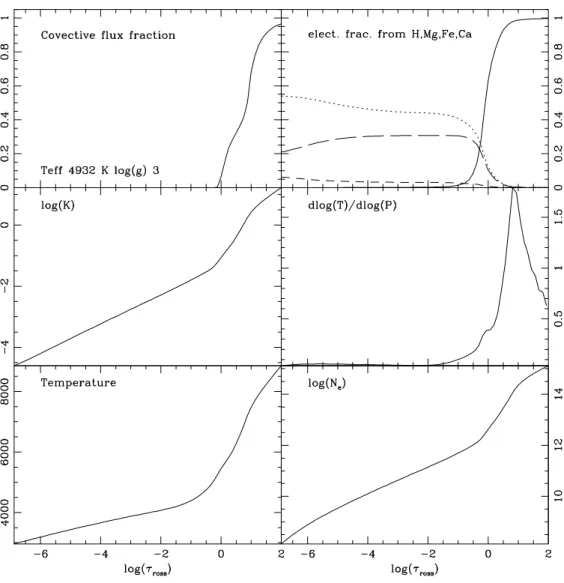
dSph galaxies (circles) and Galactic stars (triangles, Gratton et al. (2003)) . . . 30 2.1 Graphics for a model with T=4932 K,log(g) = 3, and

compo-sition scale factor of 0.31623. See text for details . . . 38 2.2 For the same model in fig. 2.1 Temperature, pressure and

thermal gradient against log(τross). . . 39

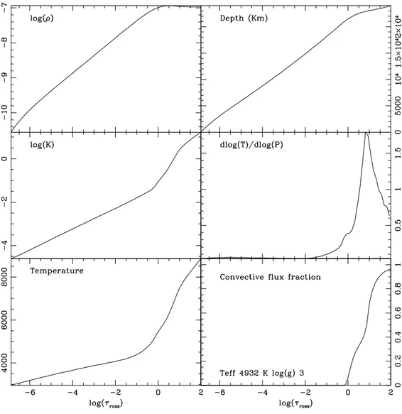
2.3 Same as in fig. 2.1, but with mass density and metric depth of the model in the two upper panels. . . 40 2.4 For the same model in fig. 2.1, the percent error over flux and

flux derivative constancy and the thermal gradient are plotted against log(τross). . . 41

2.5 Comparison between the thermal gradients of the four models, plotted against log(τross). . . 42

(10)

10 LIST OF FIGURES

2.6 Confrontation between the adiabatic thermal gradients for the four models, against log(τross) . . . 44

2.7 Confrontation between the thermal gradients of the four mod-els, plotted against ρx. . . 45

2.8 Confrontation between the thermal gradients of the four mod-els, plotted against the depth in kilometers from the outermost layer of the model. . . 46 2.9 Confrontation between the electronic numeric densities of the

four models, plotted against log(τross). . . 48

2.10 Confrontation between the mass densities of the four models, plotted against log(τross). . . 49

2.11 Confrontation between the Rosseland mean opacities of the four models, plotted against log(τross). . . 50

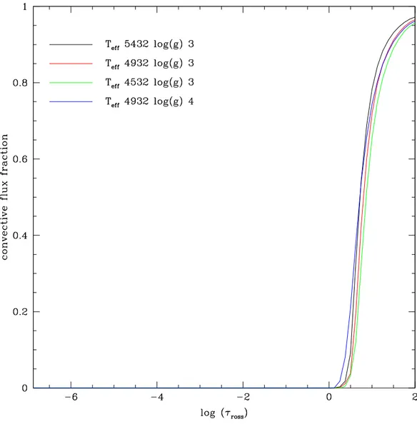
2.12 Confrontation between the fraction of fluxes transported by convection in the four models, plotted against log(τross). . . . 51

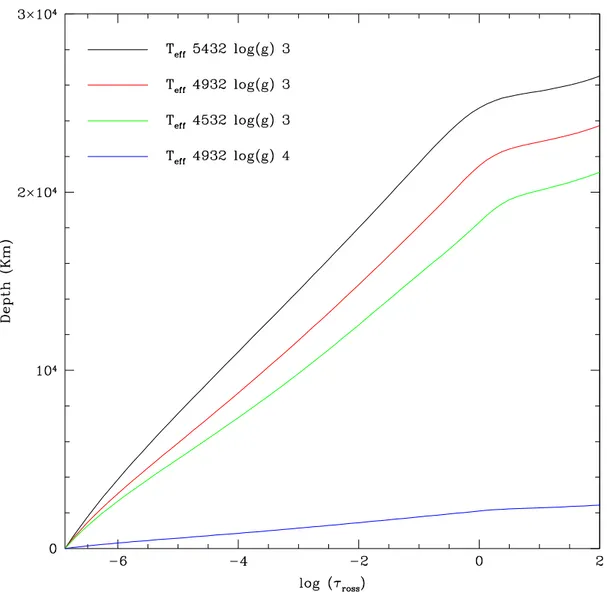
2.13 Confrontation between the metric depths in the four models, plotted against log(τross). . . 52

2.14 Confrontation between the temperatures in the four models, plotted against log(τross). . . 53

2.15 Same plots as in fig. 2.1, but for a model with Tef f 4932 K,

log(g) = 3 and overshooting. . . 54 2.16 Same plots as in fig. 2.3, but for a model with Tef f 4932 K,

log(g) = 3 and overshooting. . . 55 3.1 Plot of T against log(τRoss) along the atmosphere of a star

of Tef f = 5000 K, log g = 2.5, [F e/H]=-0.5, as produced by

the Linux ported code (solid line) and the original VMS code (triangles). . . 66 3.2 Synthetic spectrum for the above mentioned star around the

Mg b triplet. Open squares is VMS original code, solid line Linux code. The resolution of the calculation is 600000, then a gaussian broadening (7 km/s FWHM) has been added to simulate the output of a spectrometer with resolution of about 43000. An example of line label: 518360 = 518.360 nm; 1200 = Mg (12 atomic number) neutral (00); 2 = 2% residual intensity at line center (unbroadened spectrum); AZ is a code for the line log(gf ) source. . . . 67

(11)

3.3 Same as in fig. 3.1, but now comparing electron number den-sities. . . 68 4.1 Sample from the Mg b triplet region for the 12 stars of Sgr

dSph. Spectra are normalized to one on the continuum, but shifted vertically to make the figure readable. Each spectrum is shifted of 1.5 with respect to the one blow it, such as the continuum of Sgr 432 is at residual intensity of 1, for Sgr 867 is at 2.5, for Sgr 635 is at 4 and so on. Spectra are ordered such that metallicity increases ascending in the plot, every one is labeled with the star number and the [Fe/H] of the star. . . . 76 4.2 The overall plot of the chemical “signature” of the analyzed

population in Sgr dSph. [X/Fe] ratios are here plotted against atomic number. Blue symbols represent neutral elements for which [X/FeI] is plotted, while red symbols represent ionized elements, for which [X/FeII] is displayed. . . 80 4.3 CMD of the Marconi et al. (1998) photometry of Field 1,

with superimposed the program stars (filled dots) and three isochrones from the Padova series (Girardi et al., 2002) for the metallicities found in the sampled population. Adopted reddening E(V-I)=0.22, AV=0.55, and distance modulus

(m-M)=16.95 from Marconi et al. (1998). . . 86 4.4 Distribution of metallicity for the 12 UVES stars in Sgr dSph. 87 4.5 Updated version of fig. 1.1. Here the new Sgr dSph α elements

values here presented (black filled dots). Blue open circles re-fer again to stars in the Local Group dwarf spheroidals, Draco, Ursa Minor, Sextans from Shetrone, Cˆot´e, & Sargent (2001), Carina, Sculptor, Fornax and Leo from Shetrone, Venn, Tol-stoy, Primas, Hill, & Kaufer (2003). Red open triangles rep-resent the MW sample of Venn et al. (2004), comprising the Gratton et al. (2003) sample already presented in fig. 1.1. . . . 103 4.6 In top-left panel, [α/Fe] for the 12 Sgr dSph stars, plotted

against [Fe/H]. Here we define [α/Fe] as the weighted mean of [Mg/Fe], [Si/Fe] and [Ca/Fe], which are plotted, again versus [Fe/H] in the remaining three panels. [α/Fe] appear to have a decreasing trend with increasing metallicity, and remains sub-solar or solar down to almost [Fe/H]=-0.8. . . 104

(12)

4.7 [O/Fe] and [Ti/Fe] ratios for the 12 stars of Sgr dSph plotted against [Fe/H]. . . 105 4.8 Spectral syntheses for the Cu I 510.5 nm line in stars 628 and

635. . . 105 4.9 [Mg/Ca] ratio for Sgr dSph, after the new measurements (black

filled dots with error bars), for stars in the other LG dwarf spheroidals (blue open circles, same sample used in fig. 1.1 and 4.5, and for the sample of MW stars from Venn et al. (2004) (red open triangles). . . 106 4.10 Na, Al and Sc ratios with Iron, against [Fe/H], in the Sgr dSph

sample. For Na and Al ratios against Fe I are plotted against [FeI/H] while for Sc we plot [ScII/FeII] vs. [FeII/H]. Notice the [Fe/H] range is larger for the Sc plot. . . 107 4.11 [X/Fe] vs.[Fe/H] for V, Cr, Mn and Co in the sampled stars.

V, Mn and Co are neutral, Cr is ionized, so Fe II is used instead of Fe I and the [Fe/H] range is different. . . 108 4.12 Same than in fig. 4.11, for Ni, Cu and Zn. . . 109 4.13 [X/FeII] vs. [FeII/H] for species Y II, Ba II and La II in Sgr

dSph. . . 110 4.14 [X/FeII] vs. [FeII/H] for species Ce II, Nd II and Eu II in Sgr

dSph. . . 111 4.15 Comparison of Sgr dSph and Pal 12 on the [X/Fe] vs. [Fe/H]

for light odd elements Na and Sc. Big star symbol is the mean value for four Pal12 giants from Cohen (2004). . . 112 4.16 Like in fig. 4.15, but now for α elements Mg, Si and Ca. . . . 113 4.17 Like in fig. 4.15, but now for Fe-peak elements Ni, Cu and Zn. 114 4.18 Like in fig. 4.15, but now for heavy n-capture elements Y, La,

Eu. . . 115 4.19 Selection of the targets for the FLAMES analysis. Dark dots

represent the targets considered Sgr dSph members, light dots the ones that resulted to be non members. . . 116 4.20 Histogram of the entire FLAMES sample presented in Zaggia

et al. (2004). The peak of the distribution is around [Fe/H]=-0.5, the secondary peak around [Fe/H]=-1.5 is due to M54 stars. Separate histograms are presented for stars within and outside 7.5 arcmin from the M54 center. . . 117

(13)

4.21 Spectra of stars showing high velocity Na I D absorptions. The dashed-dotted line is the synthetic IS fit whereas the contin-uous line is the synthetic stellar spectrum. The local compo-nents in star # 635 are severely contaminated by telluric lines and the fit was not reliable. . . 118 4.22 A map of the position in the sky of the 12 Sgr dSph main

body stars, with indicated the two stars along which line of sight high velocity interstellar absorption components have been identified. The coordinates of the field center are indicated.119 5.1 A sample of the spectra of the five stars in the wavelength

range 601 to 605 nm, where many used Fe I features are. For star # 1282 the DIC1 spectrum is shown. . . 128 5.2 Atmospheric models for star # 1665. All models correspond

to Tef f= 3945 K log g = 0.70. The solid lines refer to an

opac-ity sampling ATLAS 12 model with abundances as provided in table 5.5. The dashed lines refer to an ATLAS 9 model computed with a solar-scaled ODF with [M/H]=-0.5 and a mi-croturbulence of 1 kms−1. The dash-dotted lines refer to the ionization structure of the above ATLAS 9 model computed by WIDTH when the abundances of table 5.5 are provided as input. The top panel shows the Fe I and Fe II ions, the middle panel the Mg I and Mg II ions, while the bottom panel displays the temperature structure of the model. The neutral ions show a peak in number densities around log τross ∼ −1.5. 136

5.3 On the left, [S/Fe] vs. [Fe/H] for the three stars of Terzan 7 and the sample of galactic stars of Ecuvillon et al. (2004). The three stars are indicated by letters: # 1665 is D, # 1282 is E and # 1708 is F. On the right, S/O vs. Oxygen content for the three Terzan 7 stars and for the galactic and extragalactic HII regions from the samples of Garnett (1989) and Izotov & Thuan (1999). The solid line represents the solar value, where A(S)¯=7.21 (Lodders, 2003) and A(O)¯=8.72 (Asplund et al.,

2004a). . . 138 5.4 Best fit of the 922.8 nm S I line for the stars # 1665, # 1282

and # 1708 (top to bottom). This is the only of the three line to be not contaminated by telluric or CN features. . . 139

(14)

5.5 [X/Fe] against [Fe/H] for the light odd atomic number ele-ments in Terzan 7(filled dots), compared to the ones presented in chapter 4 for Sgr dSph main body (open dots). Also, for comparison we include the mean value of the three stars from Tautvaiˇsien˙e et al. (2004) (large open star). As usual, ratios against Fe I are presented for neutral species, while for ionized species the comparison is made against Fe II. . . 141 5.6 As in figure 5.5 but now for mean α elements and Mg, Si and

Ca: this figure resembles directly fig. 4.6. . . 142 5.7 As in figure 5.5 but now for Fe-peak elements Ni, Cu and Zn. 143 5.8 As in figure 5.5 but now for heavy n-capture elements Y, La,

Nd and Eu. . . 144 5.9 Comparison of our measured EWs with the ones of

Taut-vaiˇsien˙e et al. (2004), for Fe, Mg, Si and Ca lines. Open hexagons refer to star 1282, crosses to star 1665, asterisks star 1708. The line is not a fit, but simply the bisector. . . 147 6.1 The EIS CMD of NGC 2477 inside which Bellazzini et al.

(2004) identified the CMa population. The selected FLAMES targets are indicated by large dots, the three likely CMa mem-bers UVES stars (see 6.3) are indicated by open stars. . . 158 6.2 Spectra of the three most probable CMa stars, in the region

of the Mg b triplet. [Fe/H], log(g) and Tef f all increase from

bottom to top. The spectra are normalized to one, stars 30077 and 6631 are shifted vertically for display purposes (continuum is at 2.5 for 30077 and at 4 for 6631). . . 159 6.3 Abundance ratios against iron plotted vs. [Fe/H] for the light

odd elements Na, Al and Sc in the three possible CMa mem-bers. . . 160 6.4 Like in fig. 6.3, for mean α elements abundance and Mg, Si

and Ca. Here we use a single figure due to the small number of stars. The filled circles with error bars represent the mean

α elements abundance similar to the one in the up-left panel

of fig. 4.6, while triangles, squares and open circles represent Mg, Si and Ca respectively. Error bars for the single elements removed for clarity. . . 161 6.5 Like in fig. 6.3, for Fe-peak elements Ni and Cu. . . 162

(15)

6.6 Like in fig. 6.3, for heavy n-capture elements Ba, La, Ce and Nd. . . 163 6.7 Synthesis for the Cu I 510.5 nm line in EIS 6631 (thick line)

with superimposed the observed spectrum. Hyperfine splitting is taken into account, [Cu/Fe]=+0.25 in the synthesis. . . 164 6.8 Metallicity distribution of the giants in the GIRAFFE sample

(red shaded histogram). The green histogram is a realization of the Besan¸con model of the Galaxy, rescaled to the observed number of objects. . . 165 6.9 Radial velocity distribution of the sample giant stars (red

shaded histogram), of the predicted stars of the Besancon model (green) and of the sample dwarf stars (blue). . . 166 6.10 The [Fe/H] vs. Vrad distribution of the observed FLAMES

giants. The red dots are the GIRAFFE targets, the three stars represent the UVES candidate CMa members, the green contour lines are the isodensity curves of the Besancon MW model. The two vertical dashed lines include the radial veloc-ities within which we estimate that MW contamination to the CMa population should be below 30%. . . 167 6.11 Radial velocity vs. galactic longitude plot for different

ob-jects of interest. Open dots mark open clusters, asterisks are globular clusters, crosses mark the velocity measurements for the recently discovered H I outer spiral arm (McClure-Griffiths et al., 2004); magenta squares represent the Yanny et al. (2003) measurements of the Monoceros Ring, the blue star is the last CMa measurements by Martin et al. (2004b), the red dot is our possible CMa component. The green lines show the expected velocity for a component in circular motion at 220 kms−1 at 15 Kpc from the center of the Galaxy. . . 168

(16)

(17)

List of Tables

3.1 Execution time comparison for ATLAS 9, calculated on 135 iterations of a 72 layers model (time per iteration within paren-theses), and for the calculation of a 5 nm synthetic spectrum at resolution 600000 with SYNTHE. Systems are: VMS: Al-phaServer 800 5-500; Pentium 4: 1.9 GHz 768 Mb RAM kernel 2.4.18-3 (Red Hat 7.3) IFC 7.0; Pentium M: 1.6 GHz, 512 Mb RAM kernel 2.4.22-1.2115.nptl (Fedora Core 1) IFC 8.0. All times in seconds. . . 65 4.1 Position, photometry, S/N ratios 580 nm and atmosphere

pa-rameters for the 12 Sgr dSph stars. . . 75 4.2 Abundances for the first 6 Sgr dSph stars. . . 81 4.3 Abundances for the other 6 Sgr dSph stars. . . 82 4.4 Ratios against Iron for the first 6 stars. [X/FeI] is used for

neutral ions, [X/FeII] for the ionized ones. For Fe I and Fe II [Fe/H] is displayed instead. . . 83 4.5 Ratios against Iron for the other 6 stars. [X/FeI] is used for

neutral ions, [X/FeII] for the ionized ones. For Fe I and Fe II [Fe/H] is displayed instead. . . 84 4.6 Atomic data, measured EWs, sources of the atomic data and

derived abundances for the measured lines, for stars 439, 628, 635 and 656. “Syn” means that the line has been measured by synthesis (no EW provided), “HFS” that hyperfine splitting has been taken into account in the synthesis, so no EW is given, and the log gf is of limited significance. For the meaning of the log gf source references see table 4.12. . . 120 4.7 Continued from table 4.6. . . 121 4.8 As in table 4.6 for stars 709, 716, 717, and 772 . . . 122

(18)

18 LIST OF TABLES

4.9 Continued from table 4.9 . . . 123 4.10 As in table 4.6 for stars 867, 879 894 and 927 . . . 124 4.11 Continued from table 4.10 . . . 125 4.12 Bibliographic reference for the log gf sources cited in tables

4.6 through 4.11, 5.2 through 5.4 and 6.5 through 6.7. . . 126 5.1 Photometry and physical parameters for the five stars. . . 129 5.2 Iron lines for the five Terzan 7 stars. For other elements see

tables 5.3 and 5.4, please refer to table 4.12 for the reference of the log gf sources. . . 131 5.3 Other elements lines for the five stars (see also tab. 5.2, 5.4).

For the three Sulphur lines, in each star equal abundances are given for all the lines, since they have been fitted together (see 5.3.1). . . 132 5.4 Other elements lines for the five stars (see also tab. 5.2, 5.3) . 133 5.5 Abundances for the Terzan 7 stars, and assumed solar

abun-dances. . . 145 5.6 Ratios against Iron for the Terzan 7 stars. [X/FeI] is used for

neutral ions, [X/FeII] for the ionized ones. For Fe I and Fe II [FeI/H] and [FeII/H] is presented. . . 146 6.1 Photometry and physical parameters for the three stars. . . . 150 6.2 Abundances and assumed solar abundances for the three likely

CMa members. . . 151 6.3 Abundance ratios for the three stars. [X/Fe I] is used for

neutral elements, [X/Fe II] for ionized species, and [Fe/H] for Fe I and Fe II. For Fe I and Fe II, [FeI/H] and [FeII/H] are presented. . . 152 6.4 Abundance ratios in different Galactic components, from Venn

et al. (2004). . . 155 6.5 Employed iron lines, atomic data, EWs and resulting

abun-dances for the three likely CMa overdensity members. Other ions, see tables 6.6 and 6.7. For the log gf references see table 4.12. . . 169 6.6 Employed lines, atomic data, EWs and resulting abundances

for ions from Na I to Mn I, for the three likely CMa overdensity members. For iron lines see table 6.5, for ions between Co I and Eu II see table 6.7. . . 170

(19)

6.7 Employed lines, atomic data, EWs and resulting abundances for the three likely CMa overdensity members, for ions between Co I and Eu II. See also tables 6.5 and 6.6. . . 171

(20)

(21)

Chapter 1 Introduction

Up to a few years ago while the Milky Way could be studied in great detail, on a star by star basis, our knowledge of external galaxies had to be desumed mainly from integrated light properties. The advent of 8m class telescopes has changed the situation dramatically, at least for Local Group (LG) galax-ies, which can now be studied on a star by star basis with the same methods previously applicable only to Galactic stars.

Dwarf galaxies in the LG are interesting objects to study for a number of reasons. The most trivial is that they are our nearest neighbors, i.e. the ones which we may study more easily. More important they constitute a natural laboratory where to study the galaxy-satellite interaction. In particular, they have been considered, since the formulation of the hierarchical galaxy forma-tion scenarios (White & Frenk, 1991; Navarro et al., 1995), as the most likely “building blocks” out of which larger galaxies, like the Milky Way, have been assembled. We will see later on how, nowadays, this interpretation should be (at least partly) rejected, since clear signs exist that present day dwarf galaxies have significantly evolved from the time of the merging phase that, in the cited scenario, built the giant galaxies. As a consequence, they may now retain only part of the characteristics of the aforementioned “building blocks”. Nevertheless, some of them have likely contributed to the formation of the Galactic Halo, and, as the case of the Sagittarius dwarf Spheroidal galaxy (Sgr dSph) strikingly shows (Majewski et al., 2003), they are still heavily contributing to shape it.

Dwarf galaxies seem also to dominate the luminosity functions, at least by numbers, both in the field (Zucca et al., 1997) and in galaxy clusters (Trentham (1998)). Moreover, their actual contribution to the cluster

(22)

22 CHAPTER 1. INTRODUCTION

ulation may still be underestimated, as suggested by the recent discovery of important populations of Ultra Compact Dwarf (UCD) galaxies inside some rich nearby clusters (Like Virgo and Fornax, see Drinkwater et al. 2003). These objects are likely the residuals of nucleated dwarf galaxies that lost their envelope in the strong gravitational fields of the central parts of these rich clusters (Bekki et al., 2003), a mechanism invoked, in the LG, also to explain the genesis of ω Centauri (Tsuchiya et al., 2004).

Finally, we will see that there is an intriguing resemblance between LG dwarf spheroidals and the Damped Ly-α systems.

1.1 Abundance analysis in dwarf galaxies with

high resolution spectroscopy

The topic of this thesis is the chemical abundance analysis in stars of the Sgr dSph and of the recently discovered Canis Major Dwarf galaxy (CMa). High resolution studies are the only ones able to produce abundance ratios for a large number of ions, far more rich in information than a mean “metallicity” (see 1.2). Just to cast an example, only detailed abundance analysis can determine the [α/Fe] ratio of a given population, which can significantly affect color magnitude diagram (Cassisi et al., 2004).

Shetrone et al. (1998) should be credited for initiating this field; with a bold leap they used the Keck telescope and the HIRES spectrograph to observe four giants in Draco. The spectroscopic metallicities confirmed what was suspected from photometry, namely a large spread in [Fe/H] ranging roughly from -3.0 to -1.4. One of the most exciting results of these pioneering observations was the discovery that the ratio [Ca/Fe] was almost solar even at very low metallicities, in stark contrast with what observed in Galactic stars.

Right from its commissioning also UVES (Dekker et al., 2000) at the VLT began to provide its contribution, by observing two giants in Sagittarius (Bonifacio et al. (2000a)). Also in this case the results were quite exciting, unveiling the existence of a rather metal-rich population ([Fe/H]∼ −0.25) which was not at all expected from the photometric studies.

It was thus clear from the beginning that the use of high resolution spec-troscopy was providing new insight into these galaxies and the time invest-ment in 8m telescopes was really quite fruitful. We now have available

(23)

abun-dances based on high resolution spectra for 8 LG dwarf spheroidals: Draco (Shetrone et al. (1998, 2001)), Sextans, Ursa Minor (Shetrone et al. (2001)), Sagittarius (Bonifacio et al. (2000a); McWilliam et al. (2003); Bonifacio et al. (2004)), Sculptor, Fornax, Carina and Leo I (Shetrone et al. (2003)). The strategy of the various groups has been different, while Shetrone and col-laborators tried to observe a few stars in as many galaxies as possible, the groups working on Sagittarius, probably driven by the complexity of this galaxy, tried to obtain data for large samples of stars in one galaxy. It is clear that both approaches have their merits and drawbacks and are highly complementary. Hopefully in a few years time we shall have large samples of stars in each of a large number of galaxies, however already the presently available data allows to draw an interesting picture of the chemistry of LG dwarf spheroidals.

1.2 Production channels for different elements

In order to interpret the evolutionary meaning of the abundances (and abun-dance ratios) we observe in dwarf galaxies, it may be useful to briefly resume the physical mechanisms through which the different elements are formed in the stellar interior, and relased in the interstellar gas. We will not enter in detail of all the nucleosynthesis process, but will instead limit us to the species that are more easily and typically measured in giant stars, the main targets of high resolution spectroscopy in the dwarf galaxies.

1.2.1 Light odd elements

Among them, the most easily measured in giants are Na (Z=11), Al (Z=13) and Sc (Z=21). Their production channels are diverse, and still open to debate. Their are produced mainly in both hydrostatic and explosive burn-ing inside massive stars explodburn-ing as SN II: Na is produced mainly in the C-burning shell, by balancing 12_C(12_C,p)23_{Na with} 23_Na(p,α)20_{Na , Al in}

the same site, where it is created from Mg (26_Mg(p,γ)27_{Al) and partially}

converted in Si (27_Al(p,γ)28_{Si) (Limongi & Chieffi, 2003; Chieffi & Limongi,}

2003, 2004). Nevertheless, some impact from proton capture processes (e.g. NeNa cycle) may influence their abundances, thus leading possibly to explain the Na-O anticorrelation observed in the Globular Clusters (GC).

(24)

1.2.2 α elements

The even atomic number elements from 8 (Oxygen) to 22 (Titanium), are generally referred to as “α elements”, since their dominant isotopes are al-ways multiples of 4_{He nuclei. By far the easiest to measure in giant stars}

spectra are Mg, Si Ca and Ti. O presents consistent observative challenges, due to the fact that its only two optical lines are forbidden and extremely weak.

In general, α elements are produced inside massive, short lived stars (with a maximum impact on the chemical enrichment due to ∼ 25M¯ stars, see

Limongi & Chieffi 2003), and then relased during the successive SN II ex-plosion. As a consequence, α elements enrichment is considered to be an extremely fast process inside a stellar population, since the lifetime of such massive stars is negligible compared to the one, e.g., of a ∼ 1M¯star. For the

same reason, α elements enrichment rate drops quickly if the star formation stops in the population.

The production channels are somewhat diverse: O (Z=8) and Mg (Z=12) are produced during hydrostatic4_{He (for O) and} 12_{C and} 20_{Ne (for Mg) core}

burning in the late stages of massive stars (Limongi & Chieffi, 2003; Chieffi & Limongi, 2003); In fact, since O burning subsequently reprocesses the Ne-burning shell, almost all the Mg produced during hydrostatic Ne Ne-burning gets destroyed. Significant quantities of Mg are also produced during explosive Ne burning, especially in low mass SN II. At the same time, both may be affected by other production/destruction channels (ON cycle, MgAl cycle, see Sneden 2004). The bulk of Si (Z=14) Ca (Z=20) and Ti (Z=22) is instead produced

probably by the so-called “α-process”, or “α”-rich freeze out”, taking place

during the actual SN II explosion, when the α-particle density is particularly high (Nakamura et al., 2001). As a consequence, although tracing the same stellar types, and consequently an overall similar evolution with time, some discrepancy may exist between different α elements (see 1.3) evolution rates. In particular, the presence or absence of hypernovae in dwarf galaxy may lead to significant changes in the [Mg/Ti] and [Mg/Ca] ratios (Venn et al., 2004, and references therein). Also, there’s the possibility that some amount of Ti and Ca may be produced by He white dwarfs exploding as SN Ia (Venn et al., 2004, and references therein). Since SN Ia are the product of slowly evolving star systems, the correlation between α elements and short lived, massive population would be weakened.

(25)

1.2.3 Iron peak elements

The elements with Z=23 (Vanadium) to 30 (Zinc) are generally defined Fe-peak elements. All of them can be measured in giant stars. Their are mainly relased in the interstellar medium (ISM) by type Ia and type II supernovae, but the variety of possible SN Ia scenarios, as well as the uncertainties in the SN II models do not allow to put too much weight in the ratios between these elements.

SN II produce important quantities of Fe peak during complete and in-complete explosive burning of28_{Si and}30_{Si (V, Cr, Mn, Co, Ni and obviously}

Fe) but the entire complete Si burning shell is believed to fall back on the compact core, and the produced elements do not pollute the ISM (Limongi & Chieffi, 2003; Chieffi & Limongi, 2004).

The simplest (and most significant) effect involving both Fe-peak and α elements is related to the fact that SN Ia do not seem to produce significant quantities of α elements (Tsujimoto et al., 1995, but see the caveat about Ca and Ti in 1.2.2). Since they enrich the ISM in Fe-peak elements, and do it on a time scale much longer than the one needed by the original α elements enrichment, the [α/Fe] ratio is seen to generally decrease with increasing [Fe/H]. As we will see later, the main factors actually determining the rate of this decrease are star formation efficiency and, in the case of dwarf galaxies, the strength of the galactic wind (Lanfranchi & Matteucci, 2004).

Another interesting effect expected to take place is the Na-Ni correlation (Venn et al., 2004, and references therein). Basically, it is due to the fact that during the SN II explosion, 58_{Ni production is favored by a neutron}

rich medium. The most common neutron rich nucleus produced by pre-SN hydrostatic burning is 23_{Na. As a consequence, Na and Ni yields from SN II}

are expected to correlate.

1.2.4 Heavy neutron capture elements

Elements above Zn (Z>30) are generally produced by n-capture processes on lighter nuclei. The most frequently observed in giant stars are Yttrium (Z=39), Barium (Z=56), Lanthanum (Z=57), Cerium (Z=58), Neodymium (Z=60) and Europium (Z=63).

Two main production channels exist for these elements. The so-called

r-process (or rapid r-process) requires a high density of neutrons, and is believed

(26)

how the mechanism of production of the elements beyond Zinc at very low metallicity is still unclear, since an heavy yield cutoff exist above Z=30 for metallicities below Z∼ 10−3 _{(Chieffi & Limongi, 2004). At increasing}

metal-licity, the r-process starts to enrich the ISM in n-capture elements. While the r-process remains the main source for some of these elements (namely Eu), at higher metallicities the s-process becomes available.

The s-process (or slow process Busso et al., 1999) is particularly efficient (among the better observable elements) for Ba, and rather efficient for Y, La, Ce and Nd. The main places where this process is believed to take place are the envelopes of low to intermediate mass AGB stars experiencing the thermal pulse phase. An alternate form (the so-called weak s-process) should take place during the hydrostatic burnings of high mass stars, but it could possibly affect only elements up to Yttrium.

At solar metallicity, almost all the Ba is produced via s-process, while 95% of Eu is still produced by r-process. As a consequence, [Ba/Eu] ratio is another signature heavily dipendent on the ration between high and low-mass, short and long lived stars. Nevertheless, strong uncertainities on the actual yelds and s vs. r contribution to many heavy elements make this signature less easy to interpret than the [α/Fe] ratio.

1.3 Observed abundance ratios in Dwarf

Galax-ies

1.3.1 α elements

In Fig. 1.1 we show the run of [α/Fe] versus [Fe/H] for the dwarf spheroidals for which data are available; α has been defined as a mean of Mg and Ca, both elements have been measured for all the observed stars. In the plot these are compared with similar data for Galactic stars (Gratton et al., 2003) and for Damped Ly-α systems (DLAs, Centuri´on et al., 2003)).

From Fig.1.1 it can be readily seen that the locus occupied by stars in dwarf spheroidal galaxies is different from that occupied by Galactic stars. On the other hand the majority of DLAs seem to fall precisely on the locus defined by dSph galaxies. The early results of Shetrone et al. (1998) and Bonifacio et al. (2000a) now appear to be a general feature of dSph galaxies: the α/Fe ratio is smaller than in Galactic stars at any given metallicity. This result was theoretically expected in galaxies which are characterized by a star

(27)

Figure 1.1: The [Fe/H], [α/Fe] diagram for stars in the Local Group dwarf spheroidals, Draco, Ursa Minor, Sextans from Shetrone, Côté, & Sargent (2001), Carina, Sculptor, Fornax and Leo from Shetrone, Venn, Tolstoy, Primas, Hill, & Kaufer (2003) Sagittarius from Bonifacio, Sbordone, Marconi, Pasquini, & Hill (2004) (open circles), Galactic stars from Gratton, Carretta, Claudi, Lucatello, & Barbieri (2003) (triangles) and for DLAs from Centurión et al. (2003) (× symbols). For the stars [α/Fe], in this plot, is defined as 0.5×([Mg/Fe]+[Ca/Fe]), for the DLAs [Si/Zn] is used as a proxy for [α/Fe] and [Zn/H] as a proxy for [Fe/H].

formation which is either slow or bursting (Gilmore & Wyse, 1991; Marconi et al., 1994; Lanfranchi & Matteucci, 2003). If, as proposed for the first time by Tinsley (1979), the pattern of α/Fe in Galactic stars is essentially due to the time delay between Type II and Type Ia supernovae, the low α/Fe values in galaxies with a slow star formation rate can be easily understood. In the Galaxy metal-poor stars are enriched mainly by Type II supernovae, while more metal-rich stars have a contribution from Type Ia supernovae, which produce large amounts of iron-peak elements, but little or no oxygen and α elements, but have longer lifetimes. When the star-formation is slow, or bursting, Type Ia supernovae have time to explode, thus pushing down the α/Fe ratio in the interstellar gas, before the next generation of stars

(28)

are formed. Thus such a galaxy should show a lower α/Fe ratio, at any metallicity, when compared to a galaxy with a continuous and rather fast star formation, like the Milky Way.

DLAs are observed as line absorption systems against the background of distant QSOs, which are characterized by large hydrogen column densities (log N > 102.3_cm−2_{, Wolfe et al., 1986). These column densities are}

charac-teristic of the disc of a spiral galaxy. It is generally accepted that the majority of the DLAs are in fact associated with galaxies of some sort, in fact they are often referred to as DLA galaxies, although, in absence of other information, one cannot exclude that any given DLA may be associated with intracluster gas or large scale filaments. Imaging studies have been able to identify the galaxies responsible for the DLA (Rao & Turnshek, 1998; Le Brun et al., 1997). For the purpose of the present discussion we shall therefore assume that DLAs are indeed galaxies. What makes DLAs very interesting is that they are observed also at high redshift (z > 3.) and it is possible to derive an accurate chemical composition, metallic lines are observed at all redshifts; no metal-free DLA has been observed to date. The lookback-time attainable through the observations of DLAs is comparable to that of old Galactic stars. The similarity of the chemical properties of most DLAs and dSphs is intriguing. One cannot conclude that most DLAs are dSphs because we know that the latter galaxies are gas-poor, while DLAs, by definition, have significant amounts of gas. One could argue that DLAs are dSphs caught in a gas-rich phase, but this is highly speculative. Instead there are two considerations which I think are fairly robust:

1. all LG dwarf spheroidals follow a similar path of chemical evolution; 2. this path is similar to that followed by DLAs.

The key to this similarity could be indeed the presence of a slow, or bursting, star formation, as suggested above. Note however that there are alternative explanations. If one admits that the initial mass function (IMF) is not the same at all times and in all places, then the increase of α/Fe with the decrease of metallicity may be interpreted as an effect of a metallicity-dependent IMF which produces more massive stars at lower metallicities. In this framework the low α/Fe in dSphs and DLAs would be the signature of an IMF which, at any metallicity, produces less high-mass stars than the Galactic IMF.

(29)

Figure 1.2: Same symbols as in as Fig.1.1, except that [Mg/Fe] and [Ca/Fe] are shown separately.

Another interesting proposal is the idea that Type Ia supernovae cannot be produced at metallicities below, roughly, [Fe/H]= −1 (Kobayashi et al., 1998, 2000). Type Ia supernovae arise in binary systems, in which a white dwarf accretes matter so as to increase its mass above the Chandrasekhar limit, thus leading to contraction and an explosion. The most popular models involve a white dwarf plus a red giant companion. In such models at low metallicities the wind of the red giants are too weak to accrete a substantial mass on the white dwarf thus the explosion stage is never reached. This scenario explains neatly the evolution of α/Fe in the Galaxy, however is unable to explain the low α/Fe ratios at low metallicities observed in dwarf spheroidals and in DLAs. Kobayashi (2003) invoked for these galaxies an IMF

(30)

Figure 1.3: The [Mg/Ca] ratio as a function of metallicity for stars in LG dSph galaxies (circles) and Galactic stars (triangles, Gratton et al. (2003)) which privileges low-mass Type II supernovae (13-15 M¯), which produce low

α/Fe ratios. This provides a viable solution, however one should be aware

that so-far in all the models of Type II supernovae the mass-cut, i.e. the mass in the SN model above which all the material is ejected and below which all material falls back on the SN remnant, cannot be determined from first principles and is therefore assumed as a free parameter (Chieffi & Limongi, 2004). A suitable choice of mass-cut may produce low α/Fe for stars of all masses. Therefore the model of Kobayashi (2003) is valid for a particular choice of (arbitrary) mass-cut.

Recently Venn, Irwin, Shetrone, Tout, Hill, & Tolstoy (2004) produced a very extensive comparison of the abundances of dwarf spheroidals with Galactic stars. On the basis of this comparison they claim that the [Mg/Fe] ratio seems to lie below [Ca/Fe] in dwarf spheroidals, while this does not seem to be the case in Galactic stars. This could be a very interesting finding, and there could be several ways to explain such behavior. The two elements Ca and Mg are produced in different sites: Mg is mainly produced by carbon burning on rather long time scales (∼ 103 _{yr) in rather deep layers, while}

Ca is produced by oxygen burning on much shorter time scales (∼ 0.3 yr) in much more superficial layers (Limongi & Chieffi, 2003). Depending on the mass-cut the ratio Mg/Ca may change. As usual also different IMFs result in different Mg/Ca ratios. The chemical evolution models of Lanfranchi & Matteucci (2004), show Ca/Fe ratios lower than Mg/Fe ratios, due to the fact that Ca and Ti are produced by Type Ia SNe more than O or Mg, thus the decrease in Ca/Fe with increasing metallicity is smaller than for Mg/Fe.

(31)

Although there are several theoretical reasons to expect this behavior, one should be cautioned that the evidence supporting this claim is still marginal. In Fig.1.2 we show the data for dwarf spheroidals and for Galactic stars, with the same symbols as in Fig.1.1. Quite obviously the scatter in [Mg/Fe] is much larger than in [Ca/Fe] however this simply reflects the observational fact that few Mg lines are measurable, while usually a larger number of Ca lines is available. If one considers all observed dSphs, except Sgr, which cover a metallicity range in which Galactic stars show a rather uniform value of [Mg/Fe] and [Ca/Fe], the mean [Mg/Fe] is 0.16 with a standard deviation of 0.2, while the mean [Ca/Fe] is 0.14 with a standard deviation of 0.11, by comparison all the Galactic stars of Gratton et al. (2003) which cover the same metallicity range (103 stars) show a mean [Mg/Fe] of 0.43 with a standard deviation of 0.11 and a mean [Ca/Fe] of 0.30 with a standard deviation of 0.08. Thus the claim that both these ratios are lower in LG galaxies than they are in Galactic stars is fairly robust, however the claim that [Ca/Fe] is lower than [Mg/Fe] among LG galaxies than in Galactic stars, is weak. This is more obvious if we look directly at the [Mg/Ca] ratio (Fig. 1.3), a larger scatter is observed , but there does not appear to be a significant difference between LG galaxies and Galactic stars.

1.3.2 Neutron capture elements

The two Sgr giants observed by Bonifacio et al. (2000a) displayed a puzzling pattern of neutron capture elements: Y appeared to be overdeficient with respect to iron, while Ba, La, Ce, Nd and Eu appeared to be overabundant. Shetrone et al. (2001) for Draco, Sextans and Ursa Minor found a similar situation: Y/Fe lower than in Galactic stars, and Ba/Fe compatible with that of Galactic stars. Now thanks to the larger data set accumulated and the precious work of Venn et al. (2004) it appears that a high [Ba/Y] and low [Y/Fe], compared to Galactic stars, is a general feature of dSphs.

There is yet no totally satisfactory explanation of this pattern, however such a behavior could be expected when neutron capture elements are pro-duced by metal-poor AGB stars, in which, due to the large neutron-to-seed ratio, the heavier elements are favored: Ba is favored over Y and Pb is favored over Ba (Busso et al. (1999)).

This cannot be the whole story, of course, because most of these stars also show [Eu/Fe] ratios which are similar or larger than those observed in Galactic stars, implying that the r−process is in operation at a level equal

(32)

or larger than what occurring in the Galaxy.

1.3.3 Undesirable building blocks

There are other elements which seem to display, at least in the case of Sagit-tarius, abundance patterns different from the Galactic ones, like Na (Boni-facio et al., 2000a), Mn (McWilliam et al., 2003) and Ni (Boni(Boni-facio et al., 2000a, , this work). The bottom line is that these chemical signatures make LG dSphs undesirable building blocks for the Galactic Halo. It is not possi-ble to assempossi-ble the Galactic Halo from dSphs with the characteristic of the present day ones. If one assumes that hierarchical galaxy formation applies to the Milky Way, one has to conclude that the dwarf galaxies which acted as building blocks were very different from present-day ones. In particular, assuming that the low α/Fe in present-day dSphs is caused by a low star formation, it can be argued the building blocks of the Milky Way where characterized by a vigorous star formation. In some sense the new informa-tion we have on LG dSphs poses more new quesinforma-tions than it answers old ones.

(33)

Chapter 2 Atlas model atmospheres

The use of a model of the stellar atmosphere is a key step in the process of interpreting stellar spectra. We call atmosphere the outermost layers of the stellar envelope, where all the spectral features (continuum and lines) originate. Here, detailed calculations are required in order to deal with the radiation transport in a optically thin, partially ionized mixture of gas. The ATLAS code simulates a one dimensional, plane parallel atmosphere under the hypothesis of flux conservation through the atmosphere. This means ne-glecting any effect related to “horizontal” motions in the atmosphere (stellar rotation, for instance). The depth of the atmosphere is also assumed to be small with respect to the stellar radius, so that the curvature of the atmo-spheric layers may be neglected, and any non-radiative heating process is set to zero: the constancy of flux through the atmosphere is assumed, no heat sources or sinks are allowed. This last limit is probably the most re-strictive, because this “energetic equilibrium” is well known to fall off in the outer solar atmosphere (the so-called transition zone to the corona) where a steep temperature increase occurs due to heating processes probably driven by seismic and magnetic waves. Another limit of such models comes from the assumption of local thermodynamic equilibrium (LTE) under which the level populations are computed1_{. In fact, there is a complex interplay}

be-tween these phenomena in the outer atmosphere of solar-like stars: NLTE processes under radiative equilibrium are partly responsible of the observed temperature rise at the bottom of the corona. Several strong spectral

fea-1_{In the codes are in fact implemented (as optional) non-LTE (NLTE) calculations for} some specific hydrogen transitions, but this is considered mainly an experimental feature, and is used only in very hot atmospheres: see Castelli (1988).

(34)

34 CHAPTER 2. ATLAS MODEL ATMOSPHERES

tures are produced in such zones, like the Ca H-K doublet core, the Hα core and the Lyman continuum. A last caveat must be made: as we will see in detail later, in ATLAS convection is treated with a “classical” mixing length approximation. In the model we shall use, overshooting is neglected, giving way to a temperature profile that is somewhat unphysical at the boundaries of the convective zone. The upper boundary of the convective layer is placed at τross > 1, so this problem will not affect strong spectral features, but will

be rather important for most weak spectral lines.

Despite of these limits, Kurucz’s models have proved to be very effective as a base for spectral analysis; their main strengths are the very detailed treatment of the bound-bound and bound-free opacity, and the very large database of atomic and molecular transition devoted to this purpose. It actually amounts to several millions of transitions, even if the physical pa-rameters are not well known for all of them, and the ones used are sometimes affected by large uncertainties. The task to deal with such a huge body of transitions is essentially impossible to address analytically, and so two main ways have been developed to practically calculate the opacity. The Opacity

Distribution Functions (ODF) method calculates explicitly the opacity for

given physical conditions, and then gives its results in a particular functional form, which allows to describe the opacity with sufficient high accuracy using a rather small dataset. The computation requires a long time, and cannot be performed during the actual model iterative calculation, so ODF are pre-calculated in a grid of different conditions, between which the values for the present model step are interpolated. The Opacity Sampling (OS) method relies on statistical methods in order to determine a sub-sample of the en-tire transition database adequate to derive the main features of the opacity. The advantage of this procedure lies in its (relative) rapidity, which allows to perform it inside the atmosphere model calculation2_{. The models used}

as examples here have been obtained using ATLAS9, the version of ATLAS code using the ODF.

2_{A description of the actual structure of both ODF and OS along with their strengths} and limits are out of the scope of the present work. A good review has been given by Carbon (1979), a detailed description of the ODF is provided by Kurucz (1979), while OS is well described, for example, by Sneden et al. (1976).

(35)

2.1 Overview of the model structure

As previously stated, ATLAS calculates plane parallel, one dimensional at-mosphere models under the hypothesis of flux conservation. The last con-dition, actually, gives the convergence parameter: the model is supposed to have converged when constancy in flux and flux derivative is assured (to a chosen cutoff) over the entire depth of the calculated atmosphere structure. The code proceeds via iterative recalculation of the physical parameters over a maximum of 72 mesh points along the atmosphere. Radiative and convec-tive energy transport are taken into account, input data to be passed to the model are effective temperature of the star, surface gravity3_{, and chemical}

composition of the gas. Usually, solar rescaled abundances are used, eventu-ally taking into account alpha elements enhancement. Additioneventu-ally, a mixing length parameter must be set to evaluate convective flux. ATLAS may take into account convective overshooting in its calculations (we will show later a model in which overshooting is employed) but not semi-convection. It must be stressed that atmospheric convection is much more sensitive to the mixing length approximation faults than core convection, since the lower opacity and viscosity enhances superadiabaticity and overshooting. A physical model of the overshooting scale, however, would require complex (and not so robust) hydro-dynamical considerations, so, if overshooting is introduced, ATLAS simply makes a smoothing of the boundaries of the convective zone on a scale of the order of the pressure scale height. This is pretty unphysical, although an abruptly ending convective layer is not much better from this point of view. Many people, anyway, prefer not to use overshooting when using ATLAS (see Castelli et al. (1997)).

Finally, a so called micro-turbulence parameter (which is dimensionally a velocity of the order of a few km/s) must be chosen, in order to ade-quately account of the non-thermal doppler broadening of the lines due to local (“turbulent”) motions in the stellar atmosphere. This last parameter, which obviously affects the opacity, is considerably important in order to derive chemical abundances from observed equivalent width of the spectral lines.

3_{In the so called “log g” form, i.e. the logarithm of the gravity acceleration in the} atmosphere: its small depth and mass compared to the whole star allow usually to consider the gravity constant along the entire model. Log(g) = 4 is typical of dwarf stars, while

log(g) = 2 ÷ 3 are the values for stars along the RGB.The gravity acceleration g is here

(36)

A starting model must be provided, and it can also be initially calculated by the program. If a database of already calculated models is available, how-ever, is customary (and generally preferable to fasten the model convergence) to start from an existent model with parameters near to the ones desired. In this hypothesis 45 to 60 model iterations are usually sufficient to reach convergence conditions not exceeding 1% maximum error in flux constancy and 10% in flux derivative constancy. The final model provides, along the 72 mesh points, the thermodynamical parameters of the gas (temperature, mass density, pressure) the ionization degree for all the elements considered in the model, electronic density, Rosseland mean opacity, convective flux fraction, depth in kilometers and so on. The program uses, as “natural” variable defining each mesh, the column density:

ρx =

Z _x

0 ρ(x)dx.

2.2 Some examples of model atmospheres

Here we present a little collection of models calculated for stars of rather low mass and metallicity, in ZAMS and RGB phases. These atmospheres have been chosen to be roughly similar to the ones we will actually encounter in our target stars, in order to give some ideas both on the way ATLAS code works and on the physics involved in such objects.

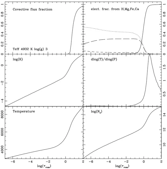
We start from a model calculated for Tef f = 4932 K, log(g) = 3 and

a solar chemical composition rescaled to 0.31623, i.e. [M/H] = −0.5 4 _.

The graphs are shown in fig. 2.1. Starting from upper left panel, are shown the fraction of the flux that is transported by convection, the contributions to the total electron density due to several elements ionization (ordered by maximum contribution: the H is the solid line, the Mg the dotted line and so on), the logarithm of the mean Rosseland opacity, the so called “thermal gradient” d log(T )_{d log(P )}, the temperature and the logarithm of the electronic density, all plotted with respect to the logarithm of the Rosseland mean optical depth. The choice of this abscissa comes from its direct dependence from the opacity and, consequently, its correlation with the energy transport mechanism.

At the first glance, a steep change may be seen in all the graphs around

τ = 1. Starting from the interior of the star we can see that, in the innermost 4_{[M/H] ≡ log(}M

H) − log(MH)¯, where M and H are the metal and H fractions, respec-tively.

(37)

layers, about all the flux is transported by convection. The opacity is at its maximum, almost all the electrons are contributed by the ionization of the hydrogen. It must be stressed that the temperature in this layer is still rater low: only roughly 10% of the H is ionized, but its high abundance makes it by far the first source of free electrons in the gas (He is essentially neutral at such temperatures). Moving outward, the efficiency of the convection decreases steeply with the optical depth of the gas and the thermal gradient increases until a maximum is reached around τ = 3. This can be seen as the point where the low opacity of the convective cells makes the convective transport essentially ineffective. Almost the entire flux is then transported by radiation, a mechanism far less efficient at such opacities. Still outward, the density and ionization continue to decrease, the atmosphere becomes essentially optically thin and the heat may be transported with higher efficiency; consequently, the thermal gradient falls off to near zero values, as the temperature decreases much more slowly than the pressure (see fig. 2.2).

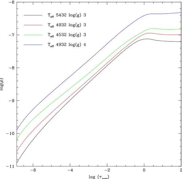
Is important to stress that the outer zone (roughly for τross < 10−4) is not

correctly modeled by ATLAS: here, as said before, the radiative equilibrium falls off and a steep temperature increase leads to the corona. All the strong spectral features at visible wavelength come from the region of (essentially flat) temperature decrease between τross = 1 and τross = 10−4. In this region,

almost all the free electrons are contributed by metallic ionization. The principal opacity source is here constituted by H− _ionization.

The steep decrease of the convective efficiency at τross ≈ 3 has to be

attributed mainly to the variation of the opacity due to a change in its source between H− _{(outward) and H ionization (inward). This may be clearly seen}

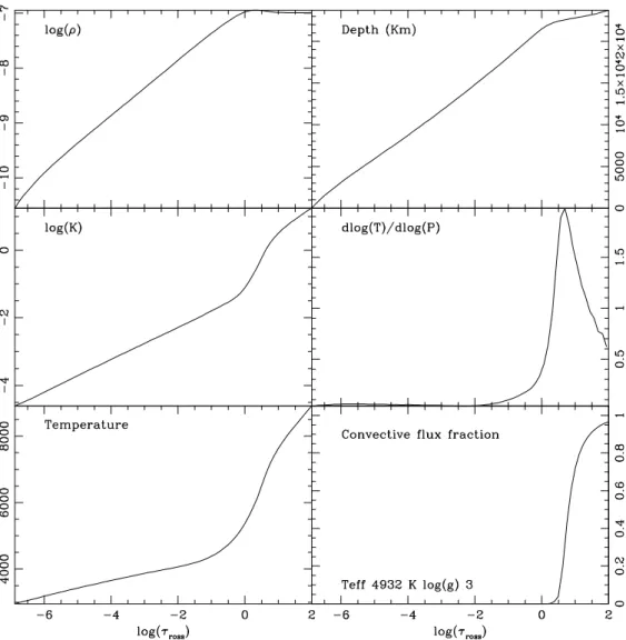
in fig. 2.3: the density, indeed, remains high and about constant until the convective flux has reached zero. Another interesting fact can be seen in fig. 2.3. The convective layer appear to be very thin, entirely contained in the last 2000 km.

Last, in fig. 2.4 we show the two errors used by ATLAS as a convergence check. Here we have plotted the (percent) deviation of the flux from the constancy, the deviation of the flux derivative from zero and the thermal gradient against log(τross). It is evident that the code encounters the biggest

problems around the peak in the thermal gradient. All the models plotted here are calculated with 60 iterations.

We will now compare this model with three others, calculated with Tef f

augmented and diminished by 500 K and with temperature unchanged, but with log(g) = 4, typical of a ZAMS star.

(38)

Figure 2.1: Graphics for a model with T=4932 K,log(g) = 3, and composition scale factor of 0.31623. See text for details

(39)

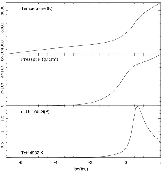
-6 -4 -2 0 2 log(tau)

dLG(T)/dLG(P)

Teff 4932 K Temperature (K)

Figure 2.2: For the same model in fig. 2.1 Temperature, pressure and thermal gradient against log(τross).

(40)

Figure 2.3: Same as in fig. 2.1, but with mass density and metric depth of the model in the two upper panels.

(41)

-6 -4 -2 0 2 log(tau)

dLG(T)/dLG(P)

Teff 4932 K Flux error

Flux derivative error

Figure 2.4: For the same model in fig. 2.1, the percent error over flux and flux derivative constancy and the thermal gradient are plotted against log(τross).

(42)

Figure 2.5: Comparison between the thermal gradients of the four models, plotted against log(τross).

(43)

First we look at the thermal gradient. Its shape appear to be very similar in all the four model, but various “scaling” differences are present. In fig. 2.5 they are plotted against log(τross); not surprisingly, the peak occurs at

very similar optical depth: the onset of convection is strictly related to the opacity. Lower temperature and higher gravity both reduce the height of the peak. Note, in fig. 2.6, the confrontation between the adiabatic thermal gradients. Formally, the so called adiabatic gradient is defined as:

∇ad = µ d log T d log P ¶ ad = P δ T ρcP

where cP is the specific heat at constant pressure and

δ = µ_{d log ρ} d log T ¶ P .

This means that its value is sensitive mainly to equation of state, chemical composition and degree of ionization of the gas. Anyway, if a perfect mono-atomic gas is assumed and any composition and ionization gradient is ex-cluded, it can be seen that the quantity assumes a constant value, ∇ad = 0.4.

The main cause of departure from this value is, in stellar atmospheres, the ionization gradients in the gas mixture: the hotter model in figure 2.6 ap-proaches better to the perfect gas in the outer layers, but it shows higher deviations in the inner zones, where H ionization becomes significant. It can be seen that, when the actual thermal gradient in the gas exceeds ∇ad, the

layer become unstable and convection sets on. In the innermost layers, a consistent depression in the adiabatic gradient contributes along with the in-creasing opacity to set on the convection. Note that the high gravity model differs here significantly from the low gravity model of same temperature, being very similar to the colder one. This can be correlated to the peaks in the thermal gradient: they are higher for the models with deeper adiabatic gradient sinks; even here, the high gravity model shows a peak much lower than the one of its low gravity “brother”, and more similar to the one of the 4532 K model.

Plotting the gradients against the column density ρx (fig. 2.7) shows

grater differences: hotter atmospheres are less dense, so, along the model, ρx

reaches smaller values. Finally, fig. 2.8 shows the gradients plotted against the metric depth of the atmosphere: the higher gravity of the fourth model leads to a far thinner atmosphere; the other three models become thicker as temperature increases, tending to “inflate” the atmosphere.

(44)

44 CHAPTER 2. ATLAS MODEL ATMOSPHERES -6 -4 -2 0 2 0 0.2 0.4 0.6 0.8

Figure 2.6: Confrontation between the adiabatic thermal gradients for the four models, against log(τross)

(45)

Figure 2.7: Confrontation between the thermal gradients of the four models, plotted against ρx.

(46)

Figure 2.8: Confrontation between the thermal gradients of the four models, plotted against the depth in kilometers from the outermost layer of the model.