UNIVERSITÀ DEGLI STUDI DI ROMA
"TOR VERGATA"
FACOLTA' DI ECONOMIA
DOTTORATO DI RICERCA IN
ECONOMIA INTERNAZIONALE
CICLO DEL CORSO DI DOTTORATO
XXII
Three Essays on International Trade
Putu Mahardika Adi Saputra
A.A. 2009/2010
Docente Guida/Tutor: Prof. Pasquale Scaramozzino and Prof. Giovanni Trovato Coordinatore: Prof. Giancarlo Marini
Three Essays on International Trade
By
Putu Mahardika Adi Saputra
SUBMITTED IN FULFILLMENT
OF THE REQUIREMENTS FOR THE DEGREE OF DOCTOR OF PHILOSOPHY IN ECONOMICS
AT
UNIVERSITY OF ROME TOR VERGATA VIA COLUMBIA 2, ROME
SUPERVISOR:
Prof. Pasquale Scaramozzino and Prof. Giovanni Trovato
Table of Contents
Table of Contents 3
Abstract 5
Acknowledgements 9
1 The dynamics of bilateral trade balance: The role of exchange rate, income and cash balance (An e mpirical case for ASEAN countries) 10
1.1 Introduction 10
1.2 Some principal facts around ASEAN trade 13
1.3 Empirical methodology 16
1.3.1 Model specification 16
1.3.2 Data source 25
1.4 Empirical results 27
1.4.1 The long run relationship 33
1.4.2 The short run relationship and the speed of adjustment 36
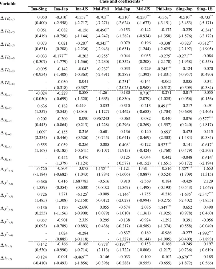
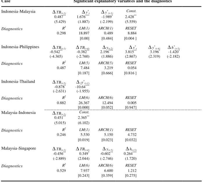
1.4.3 The estimation results of OLS 42
1.4.4 Dynamic relationships: the impulse response function and variance decomposition 48
1.4.4.1 Impulse response functions (IRFs) 48
1.4.4.1.1 Indonesia’s IRF 49
1.4.4.1.2 Malaysia’s IRF 52
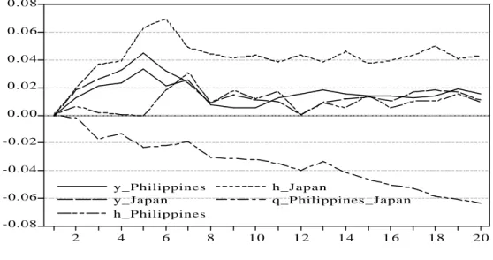
1.4.4.1.3 The Philippines’ IRF 54
1.4.4.1.4 Singapore’s IRF 55
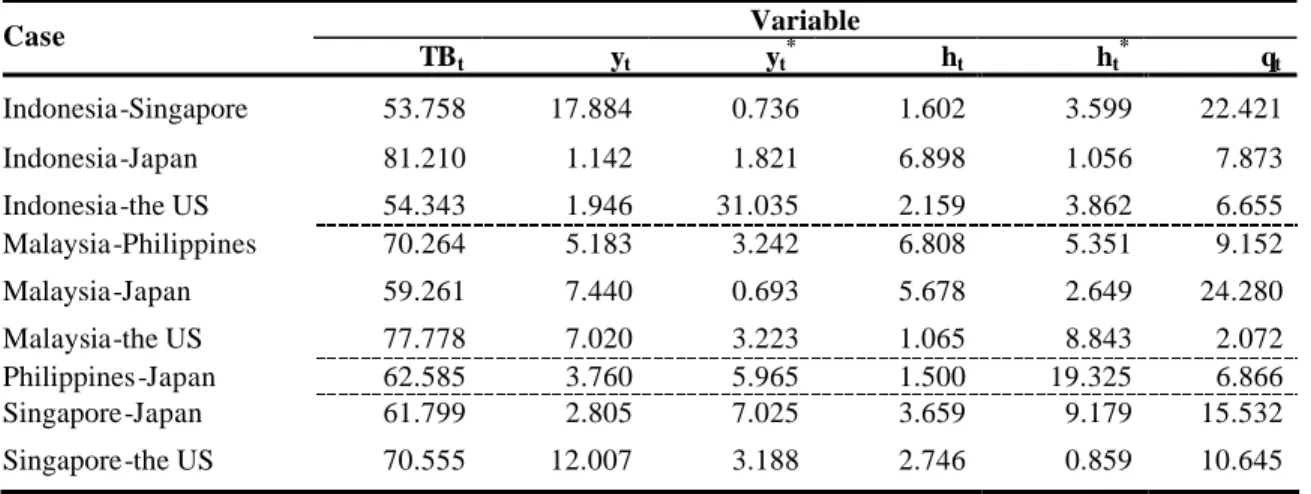
1.4.4.2 Variance decomposition 56
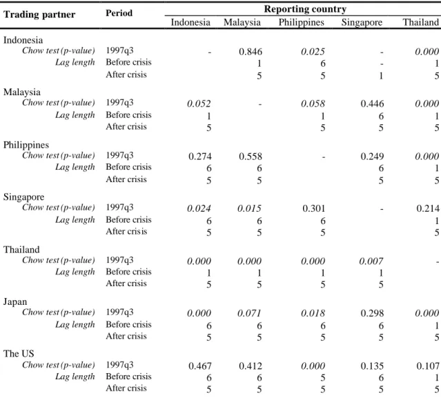
1.4.5 Is there a structural break? 59
1.4.5.1 Structural break with a known break point 60
1.4.5.2 Structural break with an unknown break point 75
1.4.5.2.1 Zivot and Andrews (1992) unit root test 75
1.4.5.2.2 Gregory and Hansen (1996) cointegration test 80
1.4.5.2.3 The long run relationship: in presence of a structural break 84
1.4.5.2.4 The short run relationship: in presence of a structural break 89
1.5 Summary of main empirical findings 93
1.6 Conclusion 96
2 Technical efficiency and export performance in Indonesian manufacturing: Evidence from sector-level data 105
2.1 Introduction 105
2.2 Empirical methodology and descriptions 110
2.2.1 Technical efficiency measurement using DEA 110
2.2.3 Export determinants: model specification and variables 115
2.2.4 The Indonesian context 117
2.2.5 Data source 118
2.3 Empirical results 120
2.3.1 DEA results 120
2.3.2 SPF results 121
2.3.3 Comparing the results 124
2.3.4 The determinants of export performance 128
2.4 Conclusion 130
3 The decision to export: Firm-level evidence from Indonesian Textile and apparel industry 141
3.1 Introduction 141
3.2 Empirical methodology 145
3.2.1 The estimating equation 145
3.2.2 Variable construction 146 3.2.2.1 Productivity 146 3.2.2.2 Size 150 3.2.2.3 Labor quality 150 3.2.2.4 Capital intensity 150 3.2.2.5 Foreign ownership 151
3.2.2.6 Region, Industry and time specific effect 151
3.2.3 Descriptive statistics 152
3.2.3.1 Data description 152
3.2.3.2 Comparisons of exporters versus non-exporters 154
3.2.3.3 Frequency of exporters and non-exporters firms 156
3.3 Empirical results 157
Abstract
This doctoral thesis consists of three independent chapters. However, those three chapters discuss a similar big issue, i.e. international trade. In depth, they talk about an empirical case of trade in Southeast Asian area (Chapter 1), and Indonesian manufacturing industries (Chapter 2 and 3). Chapter 1 will put its intention in the bilateral trade relationship among ASEAN (Association of Southeast Asian Nation) countries itself and between ASEAN and their major trading partners, Japan and the US. Chapter 2 will do an investigation on the level of efficiency of Indonesian manufacturing industries and study the determinants of export in Indonesian manufacturing. Finally, Chapter 3 observes the decision of doing export in a specific Indonesian manufacturing industry, i.e. textile and apparel firms.
In fact, we specifically put our intention on the theme of export. The discussion of it unifies those 3 chapters. However, each chapter has different emphasizes on its export idea. We stress our analysis on the effect of change in real exchange rate, real domestic income, and real domestic cash balance on the real bilateral trade balance in the first chapter, while in the second chapter; we observe the influence of capital intensity, size, export diversification and technical efficiency on the export performance, then for the last but not the least, third chapter will study the decision to export of Indonesian textile apparel firms.
Furthermore, efficiency also obtains our great concern, as we believe that efficiency is one of the important aspects that can positively affect country’s export performance (which is stated by self-selection hypothesis), thus country’s economy as well. When a firm or industry could achieve a higher level of efficiency, it should be able to enjoy a better export performance or a higher probability of becoming an exporter. More exports could be nearly related to more profit which can be collected by a firm, since export can be used by firm as a way for generating profit. Assuming firms will not do exports if they can not get any profit, then through the accumulation of the exporter’s profits, the
country’s trade balance and economy will also positively flourish. Efficiency is measured by technical efficiency in the second chapter and by total factor productivity (and labor productivity) in the third chapter. To explain shortly the discussion of the thesis, a concise description about each chapter can be shown as follows.
The first chapter examines the short run and long run effects of real exchange rate, real domestic (foreign) income, and real domestic (foreign) cash balance on the real bilateral trade balance in ASEAN region. Based on quarterly data set 1980q1 to 2007q3, investigations are carried out using VECM method. However, the impulse response functions, the variance decompositions, as well as the OLS are analyzed in order to capture further the dynamic perspective of the research. Expanding our analysis, we do test and analysis for a possibility of the presence of structural break. The Chow test is applied when a structural break with a known break point is considered. While, Zivot and Andrews (1992) unit root test, Gregory and Hansen (1996) cointegration test, and two steps Engle-Granger method are performed when a structural break with an unknown break point is measured. Results show that in the long run: (i) income effect is found to be dominant in determining the change in trade balance, either when a structural break is omitted or allowed; (ii) the cash balance effect do influence the bilateral trade; (iii) the exchange rate effect significantly plays a role only in the period before the regime shift where it is absent in the post regime shift, indicating that the structural break carries a significant impact in removing the positive long run effect of exchange rate on trade balance. With respect to that, the small economy effects are suspected to be present in ASEAN region. Meanwhile, in the short run: (i) the cash balance effect relatively plays a major role in influencing the improvement of trade balance, either when a structural break is omitted or allowed, (ii) compared to cash balance effect, the income effect is present with slightly less difference in contribution; (iii) the exchange rate effect is always observed in all types of analysis and is more discernible whe n a structural break is omitted, while a J-curve phenomenon is present in minor cases. On the contrary, once a structural break is allowed, we provide lack of evidence for the presence of the phenomenon.
The second chapter examines the technical efficiency of Indonesian manufacturing industry by estimating a stochastic production frontier (SPF) and the constant returns to scale (CRS) output-oriented DEA approach. In addition, this chapter also analyzes the determinants of export performance of the industries using panel analytical model. The results show that the estimated mean technical efficiency of Indonesian manufacturing industries which are found by those approaches are lower than 0.5. It indicates that there is substantial inefficiency problem in the industry. Comparing the scores obtained by SPF and DEA, we identify there are six relatively prominent industries in term of efficiency achievement, namely iron & steel, tobacco, transport equipment, food products, industrial chemicals, and machinery, electric. Our results which correspond to the technical efficiency indicate that the estimated mean technical efficiency in the DEA approach is larger than those obtained from the SPF. Utilizing Fixed Effect Model (FEM), we find that all export determinants, i.e. capital intensity (CAP), number of labor (SIZE), diversification (DIV) and technical efficiency (TE) shows the appropriate significant sign. The highest elasticity coefficient is provided by diversification (DIV) variable. With respect to the relationship between efficiency and export performance, we provide evidence for the presence of self-selection hypothesis.
This third chapter is devoted to the examination of factors which influence the decision to export of firms in Indonesian textile and apparel industry. Using a panel of firm- level data and a panel probit model, we test for the role of heterogeneous characteristics of firms in determining firms’ probability of exporting. We use two different definitions of firm productivity in our model, i.e. TFP and labour productivity. Besides executing the general estimation for whole observations, we execute as well the disaggregated specifications concerning the firm size (middle and large size). Mostly, the main findings in this study are in line with related previous works. In particular, we find that productivity increases the probability of exporting. Likewise, firm characteristics related to size and foreign ownership has a positive influence on the probability of exporting. On the other hand, variables accounting for capital intensity and Java region dummy affect negatively the decision to export. However, in the general estimation results, we find no significant effect of labor quality on our model. Concerning the estimation results of
disaggregated specifications, a consistent finding with the general estimation results is basically provided, except for labor quality variable which is significantly negatively related with exporting in middle-size firms’ case. This condition seemingly reflects the actual state of the textile and apparel industry in the developing economy, such as Indonesia. In which, exporters are generally inclined to be more labor intensive, and ‘cheap’ labors are specifically dominant to be employed among middle firms. Besides, the reason of less competitive in the international market also should be taken into account. Although still showing positive signs, the coefficients of productivity lose their statistical significance when the models are applied for large-sized firms. However, in general, our findings corroborate the self-selection hypothesis.
Keywords: Export, Bilateral trade balance, VECM, J-curve, Structural break, Efficiency,
Acknowledgements
This doctoral thesis has benefited very much from the help and generosity of many people. My sincere thanks go to all of them. I am particularly grateful to my supervisors, Prof. Pasquale Scaramozzino and Prof. Giovanni Trovato who kindly spared time to read my manuscripts, shared many great ideas and supported me with valuable guidance. This resulted in many comments and suggestions, which have clearly contributed to the many text improvements. I am also grateful to my external supervisor, Prof. Michael Reed (University of Kentucky) who has guided me how to create a good paper in economics area and shared much knowledge in international trade. His detailed explanations have been of inestimable value and very influential to this thesis. I would also like to thank the coordinator of the PhD program, Prof. Giancarlo Marini, for his support and advice. I would like to thank my colleagues at the Faculty of Economics, University of Brawijaya, who in all sincerity gave several ideas for the manuscripts and compelled me to think through some theoretical arguments. I am particularly indebted to the Rector of University of Brawijaya, Prof. Yogi Sugito, who has given his permission to me for studying abroad, and to the Dean of Faculty of Economic, University of Brawijaya, Dr. Gugus Irianto, who has also supported me with the faculty’s scholarship. I am also indebted to the Italian government and the University of Rome “Tor Vergata” for the scholarship assistance during my three years study period and the opportunity to expand my academic insight. Finally, I would like to acknowledge my profound gratitude to my parents, sisters (Ade and Iko), and my beloved wife, Ike Octamila, and my children, Ale and Dara. Without their spirit and support, my study and this thesis would not have been completed.
Rome, Desember 2009
Chapter 1
The Dynamics of Bilateral Trade Balance:
The role of exchange rate, income and cash balance
(An Empirical Case for ASEAN Countries)
1.1 Introduction
For more than four decades, the Association of Southeast Asian Nations (ASEAN) has been established1. So far, it is often classified as a prominent regional association in the world (see Imada, 1993; Severino, 2002; Sen, 2006). With more than 500 million inhabitants, consisting of 10 member states -Brunei Darussalam, Cambodia, Indonesia, Lao PDR, Malaysia, Myanmar, the Philippines, Singapore, Thailand and Vietnam- and whose a combined GDP around over US$ 1 trillion and total foreign trade of over US$ 1.4 trillion, in general ASEAN has became a potential partner for trading of two major economies in the world, i.e. US and Japan (ASEAN Secretariat, 2007).
After Asian financial crisis struck the region in 1997, ASEAN started to maintain intensively two fundamental internal actions in order to accelerate the recovery process and out of the downturn period rapidly. They are: first, doing intensification on trade cooperation among the member states and with other major trading partners (e.g. US, Japan, and EU); and second, doing expansion on financial cooperation among the member states itself, including China, Japan and Korea (Severino, 2002). From the first
1
ASEAN is initiated on August 8, 1967 through “Bangkok declaration” by five founding countries, i.e. Indonesia, Malaysia, the Philippines, Singapore and Thailand. In 1984, Brunei Darussalam joined ASEAN, then in 1995, 1997 and 1999, Vietnam, Lao PDR and Myanmar, and also Cambodia respectively joined.
point, we know that a consistent emphasizing on trade arrangement is still going to be a keyword and is also extremely reasonable since ASEAN has been recognized as: (i) an open organization that should liberalize its intra and inter-regional trade; and (ii) a regional bloc whose economy highly dependent on trade. With respect to the latter, Huang et al. (2004) finds that prior to the financial crisis (1996), ASEAN’s ratio of exports to GDP has achieved about 46% while the ratio of imports to GDP is around 49%. After crisis (2000), the declining of its GDP which accompanied by the growing of exports performance results in the ratio of exports to GDP increases by 71% while the ratio of import to GDP climbs to 62%. It shows the condition of ASEAN which apparently become s more trade-dependant, even after the crisis period.
The objective of this paper is to analyze the role of real exchange rates, real income and real cash balance on the bilateral trade balance among selected ASEAN countrie s (Indonesia, Malaysia, the Philippines, Singapore, Thailand) and between those ASEAN countries and the US and Japan, due to their position as the major ASEAN’s trading partners and two major economies in the world. As regarded by Tongzon and Felmingham (1998), study in bilateral trade provides a deeper insight in highlighting particular issues related to trade activity between countries, which usually are not addressed in studies of aggregate trade. Bilateral trade flows tend to respond differently to the factors (e.g. real exchange rate, income, and other monetary instruments) which determine aggregate trade flows, i.e. those variables may have different impacts on certain country where the impacts depend highly on the characteristics that owned by the country itself or its trading partner.
This paper will concentrate its discussion on ASEAN countries which are heterogeneous in numerous things, not only in cultures things, such as, languages, traditions, and religions but also in other aspects, e.g., the level of development and technology, the structure of economy, relative factor endowments and government policies. By performing particular empirical methods in the sample of heterogeneous countries, this paper expects to find interesting facts and conclusions concerning the determinants of bilateral trade, especially in each country which is analyzed.
To address the paper’s objective, a vector error correction model (VECM) is estimated. In this case, VECM treats all variables in the model as potentially endogenous. The model will analyze the impact of all considered variables on bilateral trade flows, both in the short run and long run. Additionally, the impulse response function, variance decomposition and OLS are also utilized to support the results of VECM. In order to expand our analysis, we consider the presence of a structural break. To accommodate that matter, the paper uses two types of structural break tests, namely structural break test with a known break point and structural break test with an unknown break point. Based on these tests, we investigate further whether the conclusions are sensitive to the inclusion or exclusion of a structural break.
The paper finds that in the long run, income effect is found to be dominant in determining the change in trade balance, either when a structural break is omitted or allowed. Bilateral trade appears affected too by the cash balance, and exchange rate movements. However, bilateral trade seems sensitive to bilateral exchange rate adjustments only in the period before the regime shift. The exchange rate effect is absent in the post regime shift. This condition brings us to a suspicion towards the possibility of the significant impact of financial crisis in blurring of the true relationship between real excha nge rate and trade balance.
Further, in the short run, the cash balance effect relatively plays a major role in influencing the improvement of trade balance, either when a structural break is omitted or allowed. With slightly less difference in contribution, the income effect also appears. The exchange rate effect is always observed in all type of analysis. When a structural break is omitted, the exchange rate effect is found to be more discernible. Our findings are supportive of the J-curve phenomenon in minor cases, once a structural break is neglected. However, when a structural break is allowed, we provide lack of evidence for the existence of this phenomenon. Overall, we find the exchange rate effect is sensitive to the presence of a structural break, while income and cash balance effect are less sensitive to the structural break.
The paper will be structured as follows. Section 2 discusses some principal facts around ASEAN trade. Section 3 provides the empirical methodology. While, in section 4, presents the empirical results, section 5 deals with the summary of main empirical findings, and finally section 6 concludes the paper.
1.2 Some principal facts around ASEAN trade
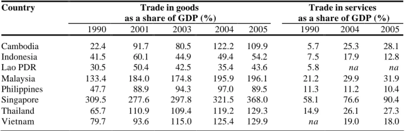
Two indicators which often used for explaining global trade and describing the importance of trade in the economy are the ratio of trade in goods to GDP and the ratio of trade in services to GDP. Trade in goods consist of all merchandise which are exported and imported by a country, while trade in services ha s a same meaning but it involves some different sectors, such as transport, travel, finance, insurance, royalties, construction, communication and cultural services (World Bank, 2006).
As seen in Table 1, the importance of trade in the economies of the region (as indicated by the ratio of trade in goods and trade in services to GDP) is quite varying for all considered periods. Singapore, one of the most open economies in the world could be expected to be superior to other economies in the region. It is verified by its ratio of trade in goods to GDP which has reached over 200%, ranging from about 277% to 368% and its ratio of trade in services to GDP which has achieved more than 50% ranging between 58% and 90%. The trades in goods/GDP ratios of other ASEAN countries move far lower than that of Singapore. The story seems still to be the same for the ratio of trade in services to GDP.
As a group, as indicated by Figure 1 and 2, the distributions of ASEAN trade are relatively concentrated in its own area. On average, during 1996-2005, intra-ASEAN trade accounted for more than 23% of export and 22% of import. Data show that intra-ASEAN trade is of growing importance, particularly for the import. Intra-intra-ASEAN import shows a gradual increase in share during 1996-2005, except for 2001, where the figure drops slightly to 21.9%. Generally, intra-ASEAN import grows from 18.4% of total in
1996 to 24.8% of total in 2005. In term of export, intra-ASEAN export always displays an increasing figure since 2001, though prior to that period, its distribution inclines to fluctuate.
Table 1. The importance of trade in ASEAN economies
Country Trade in goods
as a share of GDP (%) Trade in services as a share of GDP (%) 1990 2001 2003 2004 2005 1990 2004 2005 Cambodia 22.4 91.7 80.5 122.2 109.9 5.7 25.3 28.1 Indonesia 41.5 60.1 44.9 49.4 54.2 7.5 17.9 12.8 Lao PDR 30.5 50.4 42.5 35.4 43.6 5.8 na na Malaysia 133.4 184.0 174.8 195.9 196.1 21.2 29.9 31.9 Philippines 47.7 88.9 94.3 97.0 89.5 11.3 11.2 10.4 Singapore 309.5 277.6 297.8 321.5 368.0 58.1 76.6 90.4 Thailand 65.7 110.9 109.4 119.2 129.3 14.9 26.1 27.3 Vietnam 79.7 93.6 115.0 125.4 129.9 na 19.0 18.0
Source: World Development Indicators, 2003; 2005; 2006 and 2007, World Bank.
Notes: (1) Data are not available for Brunei Darussalam and Myanmar. (2) na means “not available”.
After ASEAN itself, developed countries are the next most significant trade partners of ASEAN. Three of them, namely the US, Japan and EU are noted as the countries whose contribution always dominate ASEAN’s export and import activities. Their contributions during 1996-2005 reach more than 11% each for both trade activities. The most dominant market for ASEAN merchandises is the US, which accounted for around 18% of total in 1996 and around 15% of total in 2005. It is followed by Japan which contributes 15% of total in 1996 and 12% of total in 2005. Meanwhile, as a group -EU market- gives its share around 14.8% on average during 1996-2005. Actually, the EU’s contribution has surpassed the Japan’s since 1997, reflecting the increasing of the importance of developed countries in Europe as the outlet for ASEAN total exports.
Developed countries are the most important import suppliers for ASEAN as well. During those periods, instead of the US, Japan places itself as the most significant key player in ASEAN market after the ASEAN countries. Even, for 1996 and 1997, the contribution of Japan is higher than ASEAN’s. In 1996, over 21% of ASEAN imports are originated
from Japan, followed by the US and EU with a similar share of around 15% each. Figure 2 presents a different tendency of contribution of intra-ASEAN imports and other three countries (the US, Japan, EU) to total ASEAN’s imports. The former tends to increase gradually during the period, and conversely, the latter inclines to decrease. Perhaps due to the deteriorating of purchasing power that encountered by ASEAN countries or due to the particular trade policy (trade agreement), for instance –in 2005-, the imports from Japan, the US and EU decline to about 14%, 11% and 13% of total, respectively. Figure 1 and 2 also describe that the import distributions of ASEAN countries match their export distributions, where similarly, they put the heaviest dependence on intra-ASEAN trading partners and then on two individual major countries, i.e. the US and Japan as their other trading partners.
Figure 1. Distribution of ASEAN exports by major destination (%), 1996-2005
ASEAN USA Japan EU 5 10 15 20 25 30 96 97 98 99 2000 01 02 03 04 05
1.3 Empirical methodology
1.3.1 Model specification
The bilateral trade balance model used is developed on the idea of Rose and Yellen (1989), Rose (1991) and Tongzon and Felmingham (1998). This paper adopts a trade balance model that relies on a standard two-country model as applied by the first two papers. However, significantly this paper also follows the work of Tongzon and Felmingham which puts the inclusion of real cash balance variable in the determination of bilateral trade flows.
Figure 2. Distribution of ASEAN imports by major destination (%), 1996-2005
ASEAN USA Japan EU 5 10 15 20 25 30 96 97 98 99 2000 01 02 03 04 05
Source: Direction of Trade Statistics Yearbook, 2003 and 2006, IMF.
As a starting point, let the paper applies two-country imperfect-substitutes model which assumes that exports and imports are imperfect substitutes for domestic goods (see Goldstein and Khan, 1985; Lindert, 1986; Rose and Yellen, 1989). On the demand side, the standard Marshallian functions which are derived from the consumer utility function
are modified with the addition of real cash balance effects. That modification is based on the work of Miles (1979) who argues that an increase of domestic real cash balance would stimulate domestic aggregate demand and increase expenditure on domestic and foreign products. This argument has been tested empirically by Bahmani-Oskooee and Malixi (1992) who have found the effect of real cash balance on import demand, notably among LDCs and by Tongzon and Felmingham (1998) who have confirmed the real cash balance effects on the bilateral trade among Australia, USA, Japan and Singapore. In this term, they justify the inclusion of the variable in our bilateral trade model. The following expressions will clarify more those points. It will be started by the equations which represent the import demand at domestic and a foreign country.
(
p y h)
p y h M M = m, , =−α1 m +α2 +α3 ………..(1)(
)
* * 3 * * 2 * * 1 * * * * * , ,y h p y h p M M = m =−α m +α +α ……….(2)Equation (1) and (2) describe the function of import quantity demanded by domestic and foreign country respectively. The dema nd for import by domestic country (M) depends negatively on the relative price of imported goods (pm) and positively on real income (y)
and real cash balance (h) while in the similar way, the demand for import by foreign country (M*) depends negatively on the foreign country’s relative import price (p*m) and
positively on foreign real income (y*) and foreign real cash balance (h*).
On the supply side, each country’s supply of exportables (X and X*) is assumed to depend positively only on the ir relative price of exportables (px and p*x) as shown by Equation (3)
and (4)2.
( )
px px X X = = β1 ………..…..……(3) 2In this case, the paper applies the argument of Bahmani-Oskooee and Kantipong (2001), Rose (1991) and Singh (2002). Their statement assumes perfect competition, in spite of there are some models of imperfect competition in supply as referred by Rose and Yellen (1989) can be utilized to get the reduced form equation.
( )
* * 1 * * * x x p p X X = = β ……..………..………(4)In the case of domestic country’s relative price, both cases, i.e. the relative price of imported goods (pm) and the relative price of exportables (px) are always measured in
domestic currency. We know that the domestic country’s relative import price (pm) is the
product of the real exchange rate (q) and the foreign country’s relative export price (p*x).
* * * * * . x x x m q p P P P P e P P e p = ⋅ ⋅ = ⋅ = ……….…. (5)
where e is the nominal or spot exchange rate where it expresses the domestic price of foreign currency and q is the real exchange rate which is defined as q =e.p* p. Meanwhile, the domestic country’s relative export price (px) is identified as the result of
the multiplication of foreign country’s relative import price (p*m) and the real exchange
rate (q). q p P P P P e P P e pm x x= x ⋅ ⋅ = ⋅ = * * * 1 1 …..……….… (6)
Due to the relative prices, then one can equilibrate supply and demand at domestic and foreign country as presented by (7).
M X M
X = *; * = ……….………(7)
The real trade balance (in terms of domestic currency), TB, is by definition expressed as the difference between the real value of export from domestic country to foreign country and the real value of import from foreign country by domestic country.
M p q M p TB x. . x. * * − = ……….……….……(8)
Equation (1) to (6) are all structural equations that can be solved together with the equilibrium conditions in (7) for the volumes and relative prices of domestic’s export and import. Through substitut ing those expressions into Equation (8), then we can find
+ − + − + + + + = * 2 1 * * 3 * 2 * 2 1 * * 1 * 2 * * 3 * * 1 * 2 1 * * 3 * 2 1 * * 1 α β α α α β α α α α α β α α β α q h q y h y q q h q q y TB + − + − + + + + − q hq q yq h y q hq q yq 2 * 1 3 2 2 * 1 1 2 3 1 2 * 1 3 2 * 1 1 α β α α α β α α α α α β α α β α ……..……(9)
Now Equation (9) may be rewritten
[
] [
]
+ + + = * 2 2 1 1 * 1 * 3 2 * * 2 * 3 2 * 2 * 1 2 * 1 2 ) ( 2 ) ( ) ( ) ( ) ( α β β α α α α β q q h y h y q TB[
] [
]
+ + + − 2 2 * 1 * 1 1 3 2 3 2 2 1 2 * 1 ) ( 2 ) ( ) ( q yhq h y q α β β α α α α β ………...(10)which can be simplified into reduced- form specification as
(
* *)
, , , ,y y h h q TB TB = ………(11)where, trade balance (TB) is expressed as a function of real exchange rate (q), the domestic (foreign) country’s real income (y, y*) and the domestic (foreign) country’s real cash balance (h, h*). According to Equation (10), TB will improve if y* and h* increase or if y and h decrease, but the influence of q still seems ambiguous.
However, there is a conventional wisdom which says that a country’s trade balance TB will improve (in the long run) when the real exchange rate q increases. The argume nt is derived from the Marshall- Lerner condition, where it states that all else equal, the trade balance will be positively affected by a real depreciation if export and import volumes are sufficiently elastic with respect to the real exchange rate, i.e. the absolute value of the
sum of the price elasticities for export and import must exceed unity (Isard, 1995; Krugman and Obstfeld, 2003)3. Assuming this condition holds, we believe that a currency depreciation will eventually lead to an improvement in the country’s trade balance.
Additionally, the literature also considers the role of time path in the relationship between the real exchange rate and trade balance. It distinguishes the time path into short and long run. Hence, after a real depreciation happens, an initial deterioration in TB occurs before an improvement is realized. This well-known phenomenon is called the curve effect. J-curve effect shows a condition where a country’s trade balance worsens suddenly after a real depreciation and improves only after a certain period of time. This effect is attributed to a lagged adjustment of quantities to changes in relative prices (Junz and Rhomberg, 1973; Pikoulakis, 1995). Basically, a real depreciation of domestic currency raises the competitiveness of prices for the domestic country’s products which then can stimulate export and reduces domestic import demand, thereby the trade balance improves. A real depreciation makes domestic products relatively cheaper than foreign products since prices of export products are sticky in sellers’ currencies. When px and p*x are assumed to
be fixed in Equation (8) and there is only a small immediate impact on the quantity of export (M*) and import (M), then we can find that the value of exports (pxM*) increases
only in a small amount, while the value of imports (qp*xM) increases significantly. This
situation results in a deterioration of trade balance in the short run. However, as time goes by for the long run, the increased price of imports brings the quantity of domestic import demand falls and due to the price elasticity of domestic export is larger in the long run than in the short run, the volume and value of domestic exports rise sufficiently to improve the trade balance so that the effect of the depreciation is cumulatively positive (Rose and Yellen, 1989; Tongzon and Felmingham, 1998; Wilson and Tat, 2001). Due to the importance of the issue, this paper decides to investigate the J-curve effect in its analysis in association with the investigation of the impact of q (the exchange rate) on TB (trade balance).
3
The exchange rate improves the bilateral trade balance if only in case Ex + Em – 1 > 0, which in turn requires Ex + Em > 1. This is a term which is known as Marshall-Lerner condition. So, when the real trade balance (TB) is initially zero, a real depreciation in domestic currency will lead to a TB surplus if the sum of Ex and Em is greater than one (Baek, 2007; Krugman and Obstfeld, 2003).
Regarding the model used, this paper starts by forming Equation (11) into a log- linear standard model and then modifies a VECM specification for the real bilateral trade balance (TB) conditional on the real exchange rate (q), real domestic (home country) income (y), real foreign income (y*), real cash balance of the home country (h), and real cash balance of the foreign country (h*). The model will be estimated in order to identify the dynamic bilateral trade relationship among selected ASEAN countries (Indonesia, Malaysia, Singapore, Thailand, and the Philippines) and between ASEAN countries and the US and Japan. The following vector error correction model (VECM) is designed for each country4: t i t k i i k t t V V u V = + + ∆ + ∆ − − = −
∑
1 1 0 δγ λ θ ……….………(12)where, Vt is the vector of endogenous variables (i.e. TB, q, y, y*, h and h*); ∆Vt is the
vector of those endogenous variables in difference; θ is (n x 1) vector of intercept terms; 0
δ is the adjustment coefficient matrix which reflects the error correction mechanism;
while the long-run equilibrium relationship between the variables are captured by the cointegrating term γVt−k; and λ is the (n x n) matrix which catches the short-run i
dynamics among variables with k-1 number of lags; finally ut is an (n x 1) vector of white
noise error terms. In addition, i and k stand for the lag order and the maximum number of the lag length, respectively. Generally, one can conclude δγVt−k as the error-correction
components and t i k i i V− − = ∆
∑
1 1λ as the vector autoregressive components in difference form.
This paper will only concentrate its analysis in variables relationship as shown by Equation (11), where all variables are expressed in natural logarithm. Real bilateral trade balance (TB) is measured as the ratio of the bilateral export value from domestic country to foreign country over the bilateral import value from foreign country by domestic country. There are two reasons why the study defines TB as a ratio of export over import:
4
First, according to Bahmani-Oskooee (1991), the ratio is insensitive to the units of measurement of export and import, whether they are measured in domestic country’s currency or foreign currency. Second, the ratio allows one to take natural logarithm of trade balance and then get the growth rates (Brada et al., 1997). Hitherto, many empirical papers in the area of the bilateral trade balance have used that ratio in their investigation, such as Arize (1996), Guptar-Kapoor and Ramakrishnan (1999), Weliwita and Tsujii (2000), Bahmani-Oskooee and Goswami (2003) and Bahmani-Oskooee and Bolhasani (2008).
After performing Equation (12), we expect the effect of domestic real income (y) to the real bilateral trade balance (TB) is negative. While, since an increase in foreign income (y*) improves TB, so their relationship should be positive5. Due to an increase in h*, which traditionally means there is an increase of foreign country’s ability to import, brings an increase in TB the n the positive sign is expected for their relationship. For h (domestic country’s real cash balance), the paper expects it to have an inverse relationship with TB.
As described in (q e p* p
.
= ); q is specified as the domestic currency price of the foreign currency. It indicates that a positive change in q implies a real depreciation of the domestic currency. If this variable gives a positive impact to TB, then one can says that the exchange rate effect is present. Marshall- Lerner condition will be satisfied, if the effect persists in the long run. Besides that, the paper will investigate deeper on the interpretation of the relationship between q and TB. That is related to an argument which is called the J-curve effect. The effect will be verified by the paper, if initially, real exchange rate (q) gives a negative impact to TB and then followed by positive impact
5
However, the relation between y and TB is still possible to be positive if: (i) increase in y is due to an increase in the production of import-substitute goods which cause the reporting country would import less, yielding an improvement in its trade balance and (ii) supply becomes the driving force in determining exports and imports (Bahmani-Oskooee and Ratha, 2004; Onofowora, 2003). By the same token, y* could also carry a negative coefficients if the increase in y* is due to an increase in the production of substitutes for reporting country’s goods which cause reporting country may export less, resulting in a deterioration of its trade balance.
after some particular periods6. In term of VECM specification, this paper also utilizes the impulse response functions for observing J-curve effect in each country.
Technically, we propose some steps in estimating Equation (12). As the first step, we do the determination of lag length for each case by employing Akaike Information Criterion (AIC) as suggested by Onafowora (2003). Then, due to the importance of the property of stationarity in a time series variable, we do the second step, i.e. the test for stationarity and unit roots of each variable by performing the Augmented Dickey-Fuller (ADF) test. A time series variable is called stationa ry if it possesses a finite mean, variance and autocovariance function which are all independent of time. Testing of unit root involves the testing of order of integration of the series. The series is said to be integrated of order
d if it requires differencing d times in order to achieve stationarity. So, a series Xt is said
to be integrated of order one, Xt ~ I(1), if its level series, Xt, is nonstationary but its
first-differenced series (∆Xt) is stationary, ∆Xt~ I(0). Using the Augmented Dickey-Fuller
test methodology, our fundamental regression equation to test unit root is:
t i t k i i t t a a y b y y = + + ∆ +ε ∆ −+ = −
∑
1 2 1 1 0 ………..………..(13)Above equation adds an intercept term to the pure random walk model which constitutes another version of the ADF test. The null hypothesis of unit root fails to be rejected if a1
= 0. If the null hypothesis a1 = 0 is rejected, the series is stationary.
After finding which series are nonstationary (in level) and have same order of integration, we test whether the linear combination of the series is stationary, i.e. they are cointegrated. Cointegration test is a test for equilibrium between nonstatio nary variables which have same order of integration. It becomes important since nonstationary variables may bring a possibility of the existence of the long-run relationship among variables in the vector auto-regression system (Engle and Granger, 1987).
6
Krugman and Obstfeld (2000), for instance, give a thorough explanation about the argument of J-curve effect
To accommodate the cointegration test for this paper, as the third stage, we perform the Johansen test. Johansen (1991) introduces two likelihood ratio test statistics for testing the hypothesis of r cointegrating vectors. They are broadly known as the trace statistic and the maximum eigenvalue statistic (λ ). The first statistic tests the null hypothesis max
r = r0 against the alternative r > r0 for r0 = (0, 1, ….., p). Where, if the null hypothesis of
at most r0 cointegrating vectors is true, then there should be p – r0 eigenvalues which are
not statistically different from zero. While, the latter tests the null hypothesis r = r0
against the alternative r = r0 + 1. In this case, if the null hypothesis is true, then we can
expect that r0 + 1 eigenvalues are not statistically different from zero. Actually, the
intuition of those tests is that since cointegrating relationships are connected with nonzero eigenvalues, thus testing the null hypothesis of r cointegrating vectors is alike to testing how many of the largest ordered eigenvalues are significantly different from zero (see Yousefi and Wirjanto, 2003).
In general, if the results conclude the absence of cointegrating vectors between the variables, it means that there is no long-run relationship among them. Conversely, if co-integration exists, then the long-run relationship among variables appears in the case and it can be presumed that a dynamic specification of the error correction mechanism is appropriate (Engle and Granger, 2000). For the last step, the paper executes the VECM in order to examine the short and long-run relationship of the model. Additiona lly, the impulse response function and variance decomposition are applied for complementing the dynamic perspective of the paper.
However, in order to expand our analysis, we investigate the short-run relationship between the trade balance and other cons idered variables for the bilateral cases which are excluded from the execution of VECM by using OLS. OLS is still employed based on Equation (11), in which all variables are treated at their appropriate integration order and optimum lag length. Furthermore, the presence of a structural break also becomes our consideration. To accommodate that matter, the paper uses two types of structural break
tests, namely structural break test with a known break point and structural break test with an unknown break point.
1.3.2 Data source
To carry out the empirical work, quarterly data for the first quarter of 1980 to the third quarter of 2007 (1980q1-2007q3) are used7. Data are collected from Direction of Trade
Statistics (DOTS) of IMF and International Financial Statistics (IFS) of IMF. The real
bilateral trade balance (TB) is measured as a ratio of merchandise f.o.b. exports to merchandise c.i.f. imports multiplied by 100. Since DOTS-IMF only covered 2003q1-2007q3 Singapore’s export-import data to and from Indonesia, then the paper will only used that series for the case without doing any techniques of data mining.
Due to the absence of quarterly GDP data in most countries during the research periods (1980q1-2007q3), following Wilson and Tat (2001), Bahmani-Oskooee and Goswami (2003) and Bahmani-Oskooee and Ratha (2004), this paper uses industrial production index (for Malaysia, Japan and the US) and manufacturing production index (for Indonesia, Philippines, and Singapore) as a proxy for the real domestic (foreign) income. All with index numbers (2000=100). Note that, since those two indexes are not available for Thailand, then this paper uses quarterly data of nominal GDP for that country but with a shorter research period (1993q1-2007q3)8. Thailand’s quarterly nominal GDP series was deflated by its CPI (2000=100) to express it in real terms. It then was expressed as an index with 2000=100.
Home country’s real cash balance (h), following Bahmani-Oskooee (1985) and Tongzon and Felmingham (1998), is obtained by adding currency outside banks (IFS, 14a) and commercial banks reserves (IFS, 20) and then deflated by the country’s CPI (IFS, 64). An
7
Note that for all Thailand cases and Singapore-Indonesia case, this paper uses quarterly data for 1993q1-2007q3 and 2003q1-1993q1-2007q3 respectively.
8
IFS-IMF data source only provides Thailand’s nominal GDP data from 1993q1 to 2007q3. Manufacturing production index data are used if a country does not have industrial production index data. For consistency, the paper uses industrial production index for Japan and the US.
equivalent procedure (as shown by h) is used to generate the foreign country’s real cash balance (h*) based on their respective data.
The bilateral real exchange rate (q) is computed by multiplying the spot or market exchange rate –e (IFS, rf) by the ratio of foreign price to the domestic price level and then multiplied by 100. Price level will be proxied by the CPI (IFS, 64). Note that, since the IMF provides all exchange rates in relation to the US dollar, then a conversion adjustment in relation to other currencies -outside the US dollar- are needed. If the bilateral exchange rate want to be generated against the Malaysian Ringgit, then domestic currency value of the Ringgit can be measured as the ratio of the domestic currency exchange rate against the US dollar to the Ringgit rate against the US dollar. Further explanation about data and variables used are summarized in Table 2. All variables are in natural logarithm form.
Table 2. Variables, definitions and data sources
Variable Definition Source
TB The real bilateral trade balance. It is measured as a ratio of merchandise f.o.b. exports to merchandise c.i.f. imports multiplied by 100. Singapore-Indonesia case (but not Indonesia-Singapore) used data from 2003q1 to 2007q3.
DoTS (Direction of Trade Statistic), IMF, various years
y(y*) The domestic (foreign) country’s real domestic income. Following Wilson and Tat (2001), Bahmani-Oskooee and Goswami (2003) and Bahmani-Oskooee and Ratha (2004), this paper uses industrial production index (for Malaysia, Japan and the US) and manufacturing production index (for Indonesia, Philippines, and Singapore) instead of real GDP. Since those two indexes are not available for Thailand, then this paper uses quarterly data of nominal GDP for the country with a shorter research period (1993q1-2007q3).
IFS (International Financial Statistics), IMF, various years
h(h*) Domestic (foreign) country’s real cash balance. Following Bahmani-Oskooee (1985) and Tongzon and Felmingham (1998), they are obtained by adding currency outside banks (IFS, 14a) and commercial banks reserves (IFS, 20) and then deflated by the country’s CPI (IFS, 64).
IFS (International Financial Statistics), IMF, various years
q The real bilateral exchange rate; it is computed by multiplying the spot or market exchange rate –e (IFS, rf) by the ratio of foreign price -foreign country’s CPI (IFS, 64) to the domestic price level -home country’s CPI (IFS, 64) and then multiplied by 100.
IFS (International Financial Statistics), IMF, various years
1.4 Empirical results
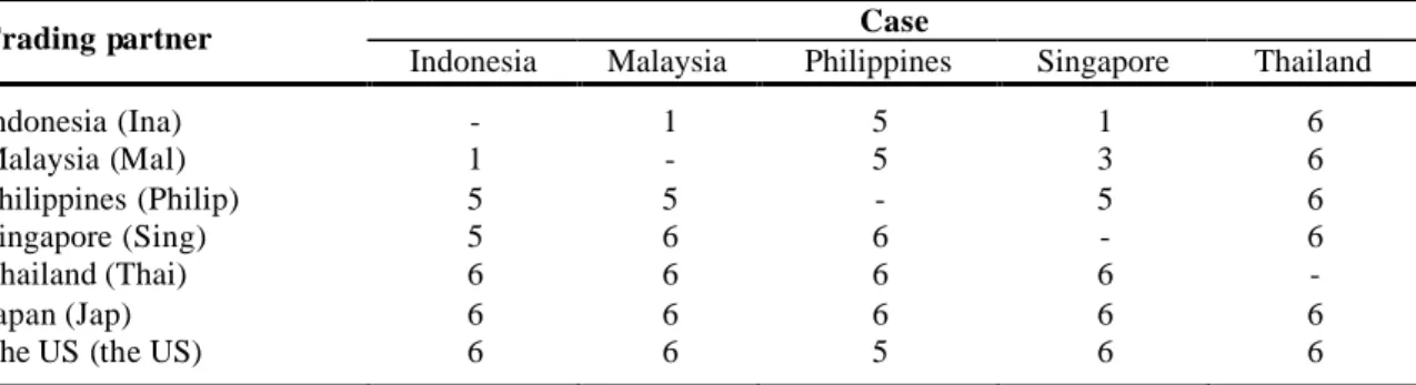
As the first step, this paper determines the lag length of each bilateral case by using Akaike Information Criterion (AIC). In order to get the optimum lag length, following Moura and Da Silva (2005), we estimate a vector auto regression (VAR) for the variables in levels, where it imposes a maximum of six lags on each variable and employs AIC to select the optimum lag length9. The results are reported in Table 3.
Table 3. The optimum lag length based on AIC for each country case
Case Trading partner
Indonesia Malaysia Philippines Singapore Thailand
Indonesia (Ina) - 1 5 1 6 Malaysia (Mal) 1 - 5 3 6 Philippines (Philip) 5 5 - 5 6 Singapore (Sing) 5 6 6 - 6 Thailand (Thai) 6 6 6 6 - Japan (Jap) 6 6 6 6 6
The US (the US) 6 6 5 6 6
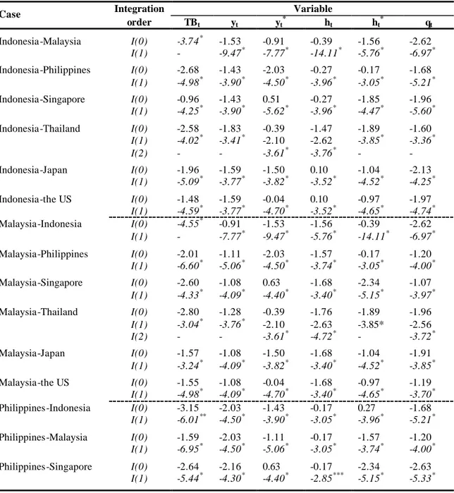
For the next step, we test for stochastic trends in the autoregressive representation of each individual time series using the augmented Dickey - Fuller (ADF) test. Through ADF, we check the variables for unit roots to examine their order of integration, since cointegration requires the variables to be integrated in the same order. For this test, intercept terms in the test regression are included.
According to Table 4, the ADF test finds two individual time series are stationary in level [I(0)], namely (i) the trade balance (TB) between Indonesia and Malaysia, and (ii) the trade balance between Malaysia and Indonesia. For the majority of remaining series, the ADF tests provide a strong indication of unit roots, in which they are [I(1)] processes in their respective bilateral case. However, there are exceptions to these ten series which are
9
Due to the limitation of data availability, the paper imposed a maximum of one lag on each variable for Singapore-Indonesia series.
stationary in second differences [I(2)], namely y data for Thailand and the US (in Thailand-US case), h data for Indonesia, Malaysia and Philippine (when they do trade with Thailand), q data for Malaysia-Thailand, Singapore-Indonesia, Thailand-Malaysia, Thailand-the US, and TB data for Singapore-Thailand.
Table 4. Summary results of unit root tests
Integration Variable Case order TBt yt yt* ht ht* qt Indonesia-Malaysia I(0) -3.74* -1.53 -0.91 -0.39 -1.56 -2.62 I(1) - -9.47* -7.77* -14.11* -5.76* -6.97* Indonesia-Philippines I(0) -2.68 -1.43 -2.03 -0.27 -0.17 -1.68 I(1) -4.98* -3.90* -4.50* -3.96* -3.05* -5.21* Indonesia-Singapore I(0) -0.96 -1.43 0.51 -0.27 -1.85 -1.96 I(1) -4.25* -3.90* -5.62* -3.96* -4.47* -5.60* Indonesia-Thailand I(0) -2.58 -1.83 -0.39 -1.47 -1.89 -1.60 I(1) -4.02* -3.41* -2.10 -2.62 -3.85* -3.36* I(2) - - -3.61* -3.76* - - Indonesia-Japan I(0) -1.96 -1.59 -1.50 0.10 -1.04 -2.13 I(1) -5.09* -3.77* -3.82* -3.52* -4.52* -4.25* Indonesia-the US I(0) -1.48 -1.59 -0.04 0.10 -0.97 -1.97 I(1) -4.59* -3.77* -4.70* -3.52* -4.65* -4.74* Malaysia-Indonesia I(0) -4.55* -0.91 -1.53 -1.56 -0.39 -2.62 I(1) - -7.77* -9.47* -5.76* -14.11* -6.97* Malaysia-Philippines I(0) -2.01 -1.11 -2.03 -1.57 -0.17 -1.20 I(1) -6.60* -5.06* -4.50* -3.74* -3.05* -4.00* Malaysia-Singapore I(0) -2.60 -1.08 0.63 -1.68 -2.34 -1.07 I(1) -4.33* -4.09* -4.40* -3.40* -5.15* -3.97* Malaysia-Thailand I(0) -2.80 -1.28 -0.39 -1.76 -1.89 -1.96 I(1) -3.04* -3.76* -2.10 -2.63 -3.85* -2.56 I(2) - - -3.61* -4.72* - -3.72* Malaysia-Japan I(0) -1.57 -1.08 -1.50 -1.68 -1.04 -1.91 I(1) -3.24* -4.09* -3.82* -3.40* -4.52* -3.85* Malaysia-the US I(0) -1.55 -1.08 -0.04 -1.68 -0.97 -1.19 I(1) -4.98* -4.09* -4.70* -3.40* -4.65* -3.70* Philippines-Indonesia I(0) -3.15 -2.03 -1.43 -0.17 0.27 -1.68 I(1) -6.01** -4.50* -3.90* -3.05* -3.96* -5.21* Philippines-Malaysia I(0) -1.59 -2.03 -1.11 -0.17 -1.57 -1.20 I(1) -6.95* -4.50* -5.06* -3.05* -3.74* -4.00* Philippines-Singapore I(0) -2.64 -2.16 0.63 -0.17 -2.34 -2.63 I(1) -5.44* -4.30* -4.40* -2.85*** -5.15* -5.33*
Table 4. (Continued) Integration Variabl e Case order TBt yt yt* ht ht* qt Philippines-Thailand I(0) -1.76 -1.75 -0.39 0.48 -1.89 -1.87 I(1) -3.07* -3.03* -2.10 -1.37 -3.85* -3.02* I(2) - - -3.61* -4.61* - - Philippines-Japan I(0) -1.86 -2.16 -1.50 -0.17 -1.04 -2.38 I(1) -4.02* -4.30* -3.82* -2.85*** -4.52* -4.44* Philippines-the US I(0) -2.23 -2.03 0.18 -0.17 -0.91 -1.97 I(1) -4.39* -4.50* -3.76* -3.05* -3.80* -4.33* Singapore-Indonesia I(0) -2.83 -1.10 -3.07 1.91 -1.72 -1.32 I(1) -3.32* -3.86* -5.18** -3.57* -4.41* -2.60 I(2) - - - -3.97* Singapore-Malaysia I(0) -1.72 0.49 -1.02 -1.81 -1.50 -1.29 I(1) -5.04* -4.02* -4.98* -5.18* -3.97* -5.05* Singapore-Philippines I(0) -1.79 0.51 -2.03 -1.85 -0.17 -2.62 I(1) -5.46* -5.62* -4.50* -4.47* -3.05* -5.51* Singapore-Thailand I(0) -0.21 0.61 -0.39 0.14 -1.89 -1.74 I(1) -2.19 -3.45* -2.10 -4.01* -3.85* -2.77*** I(2) -5.34* - -3.61* - - - Singapore-Japan I(0) -0.24 0.63 -1.50 -2.34 -1.04 -2.74 I(1) -5.20* -4.40* -3.82* -5.15* -4.52* -3.83* Singapore-the US I(0) -1.88 0.63 -0.04 -2.34 -0.97 -1.92 I(1) -4.57* -4.40* -4.70* -5.15* -4.65* -2.68*** Thailand-Indonesia I(0) -3.47 -0.39 -1.83 -1.89 -1.47 -1.60 I(1) -5.60** -2.10 -3.41* -3.85* -2.62 -3.36* I(2) - -3.61* - - -3.76* - Thailand-Malaysia I(0) -2.72 -0.39 -1.28 -1.89 -1.76 -1.96 I(1) -3.52* -2.10 -3.76* -3.85* -2.63 -2.56 I(2) - -3.61* - - -4.72* -3.72* Thailand-Philippines I(0) -2.87 -0.39 -1.75 -1.89 0.48 -1.87 I(1) -3.65* -2.10 -3.03* -3.85* -1.37 -3.02* I(2) - -3.61* - - -4.61* - Thailand-Singapore I(0) -0.57 -0.39 0.61 -1.89 0.14 -1.74 I(1) -3.51* -2.10 -3.45* -3.85* -4.01* -2.77*** I(2) - -3.61* - - - - Thailand-Japan I(0) -2.07 -0.39 0.25 -1.89 -1.44 -1.19 I(1) -3.50* -2.10 -3.04* -3.85* -3.11* -2.66*** I(2) - -3.61* - - - - Thailand-the US I(0) -1.52 -0.39 -1.34 -1.89 -1.21 -1.56 I(1) -3.47* -2.10 -2.32 -3.85* -3.24* -2.32 I(2) - -3.61* -4.47* - - -3.84*
Notes: (1) All variables in natural logarithm form. (2) These tests are carried out over the period 1980q1 to 2007q3 except for all Thailand cases which are carried out over 1993q1 to 2007q3 and Singapore-Indonesia case which are carried out over 2003q1 to 2007q3. (3) This paper tests the null hypothesis of a unit root in levels and also in first differences and second differences of variables. (4) *, ** and *** mean to reject the null hypothesis at 5%, 1% and 10% level, respectively .
Since some series are integrated of different order and we have considerable evidence that the majority of the series are getting stationary in first differences [I(1)], hence this paper only consider to identify the long-run relationships among variables for each bilateral case which are stationary at [I(1)]. All bilateral cases which posses variables that get stationary in second differences [I(2)] are excluded from the cointegration test.
Table 5. Summary results of Johansen cointegration tests
The statistic value of The p-value of
Case (r) Eigenvalues Trace
max λ Trace λmax Indonesia-Philippines r=0 0.244 87.684 29.317 0.158 0.470 r=1 0.231 58.367 27.603 0.289 0.232 r=2 0.154 30.764 17.612 0.679 0.528 r=3 0.062 13.152 6.704 0.884 0.965 r=4 0.047 6.448 5.022 0.643 0.739 r=5 0.013 1.426 1.426 0.232 0.232 Indonesia-Singapore r=0 0.398 137.009** 53.319** 0.000 0.001 r=1 0.274 83.689** 33.662*** 0.002 0.053 r=2 0.235 50.027* 28.136* 0.031 0.043 r=3 0.123 21.891 13.827 0.305 0.379 r=4 0.068 8.064 7.426 0.459 0.440 r=5 0.006 0.637 0.637 0.425 0.425 Indonesia-Japan r=0 0.303 114.386** 37.570*** 0.001 0.093 r=1 0.244 76.817* 29.120 0.012 0.167 r=2 0.178 47.697*** 20.325 0.052 0.319 r=3 0.168 27.371*** 19.089*** 0.093 0.094 r=4 0.069 8.282 7.410 0.436 0.442 r=5 0.008 0.872 0.872 0.351 0.351 Indonesia-the US r=0 0.316 123.022** 39.427*** 0.000 0.059 r=1 0.282 83.595** 34.505* 0.003 0.042 r=2 0.187 49.090* 21.476 0.038 0.249 r=3 0.142 27.614*** 15.937 0.088 0.229 r=4 0.075 11.677 8.114 0.173 0.367 r=5 0.034 3.563*** 3.563*** 0.059 0.059 Malaysia-Philippines r=0 0.326 104.313* 41.357* 0.011 0.036 r=1 0.219 62.957 25.953 0.156 0.324 r=2 0.159 37.004 18.190 0.347 0.480 r=3 0.093 18.814 10.242 0.506 0.722 r=4 0.056 8.573 5.998 0.406 0.614 r=5 0.024 2.575 2.575 0.109 0.109 Malaysia-Singapore r=0 0.285 105.238* 34.880 0.010 0.172 r=1 0.251 70.358* 30.107 0.045 0.132 r=2 0.173 40.251 19.748 0.214 0.359 r=3 0.138 20.502 15.421 0.389 0.261 r=4 0.047 5.081 4.972 0.800 0.745 r=5 0.001 0.109 0.109 0.741 0.741
Table 5. (Continued)
The statistic value of The p-value of
Case (r) Eigenvalues
Trace λmax Trace λmax
Malaysia-Japan r=0 0.309 118.733** 38.422*** 0.001 0.076 r=1 0.245 80.311** 29.161 0.006 0.165 r=2 0.219 51.151* 25.675*** 0.024 0.086 r=3 0.107 25.475 11.756 0.145 0.572 r=4 0.099 13.719*** 10.879 0.091 0.160 r=5 0.027 2.840*** 2.840*** 0.092 0.092 Malaysia-the US r=0 0.345 140.455** 43.951* 0.000 0.018 r=1 0.314 96.503** 39.166* 0.000 0.011 r=2 0.233 57.337** 27.524*** 0.005 0.051 r=3 0.116 29.813* 12.837 0.049 0.467 r=4 0.083 16.976* 9.056 0.030 0.282 r=5 0.073 7.921** 7.921** 0.005 0.005 Philippines-Indonesia r=0 0.252 76.318 30.440 0.495 0.396 r=1 0.177 45.878 20.407 0.802 0.728 r=2 0.105 25.471 11.622 0.905 0.947 r=3 0.064 13.850 6.936 0.849 0.956 r=4 0.040 6.913 4.284 0.588 0.828 r=5 0.025 2.630 2.629 0.105 0.105 Philippines-Malaysia r=0 0.257 94.950*** 31.221 0.057 0.347 r=1 0.224 63.729 26.636 0.139 0.283 r=2 0.138 37.093 15.560 0.343 0.703 r=3 0.120 21.533 13.438 0.325 0.413 r=4 0.044 8.095 4.732 0.455 0.775 r=5 0.032 3.363*** 3.363*** 0.067 0.067 Philippines-Singapore r=0 0.266 98.278* 32.129 0.033 0.296 r=1 0.211 66.149*** 24.616 0.095 0.412 r=2 0.177 41.533 20.199 0.172 0.328 r=3 0.117 21.335 12.902 0.337 0.461 r=4 0.061 8.432 6.581 0.420 0.540 r=5 0.018 1.852 1.852 0.174 0.174 Philippines-Japan r=0 0.345 118.052** 44.025* 0.001 0.017 r=1 0.282 74.028* 34.525* 0.022 0.042 r=2 0.156 39.503 17.616 0.241 0.527 r=3 0.109 21.887 12.046 0.305 0.543 r=4 0.059 9.842 6.336 0.293 0.571 r=5 0.033 3.506*** 3.506*** 0.061 0.061 Philippines-the US r=0 0.289 108.926** 35.761 0.005 0.142 r=1 0.253 73.165* 30.583 0.026 0.118 r=2 0.153 42.581 17.380 0.143 0.548 r=3 0.128 25.202 14.403 0.154 0.333 r=4 0.060 10.799 6.457 0.224 0.555 r=5 0.041 4.342* 4.342* 0.037 0.037 Singapore-Malaysia r=0 0.223 79.808 27.014 0.371 0.632 r=1 0.209 52.795 25.131 0.514 0.376 r=2 0.104 27.663 11.787 0.828 0.941 r=3 0.074 15.876 8.266 0.721 0.887 r=4 0.068 7.611 7.581 0.508 0.423 r=5 0.0003 0.030 0.030 0.862 0.862 Singapore-Philippines r=0 0.280 92.176*** 34.505 0.086 0.182 r=1 0.218 57.671 25.794 0.314 0.333 r=2 0.137 31.877 15.522 0.619 0.706
Table 5. (Continued)
Notes: (1) r denotes the number of cointegrating vector. (2) *, ** and *** denote rejection of null hypothesis at 5%, 1%
and 10% level, respectively.
So as the consequence, the paper cannot conduct cointegration test in the bilateral case of: (i) Indonesia-Malaysia, (ii) Indonesia-Thailand, (iii) Indonesia, (iv) Malaysia-Thailand, (v) Philippines-Malaysia-Thailand, (vi) Singapore-Indonesia, (vii) Singapore- Malaysia-Thailand, (viii) Thailand-Indonesia, (ix) Thailand-Malaysia, (x) Thailand-Philippines, (xi) Thailand-Singapore, (xii) Thailand-Japan, and (xiii) Thailand-the US.
This paper uses Johansen cointegration test to find out the possibility of long run relationship among the variables in each case. In applying the test, the optimum lag length employed can be different for every case. They are chosen according to the minimum AIC as reported by Table 3. Using the procedure proposed by McKinnon et al. (1999), the p-values of trace and the maximum eigenvalue test results are reported in Table 5.
Based on the computed p-values, we reject the null hypothesis of no cointegration (r=0) in 9 out of 17 cases. Those 9 cases have at least one cointegrating relationship among the variables, hence as a result; we only can apply VECM in those bilateral cases. They are: (i) Indonesia-Singapore; (ii) Indonesia-Japan; (iii) Indonesia-the US; (iv)
Malaysia-The statistic value of The p-value of
Case (r) Eigenvalues
Trace λmax Trace λmax
r=3 0.106 16.355 11.821 0.687 0.566 r=4 0.041 4.534 4.388 0.856 0.816 r=5 0.001 0.146 0.146 0.702 0.702 Singapore-Japan r=0 0.358 121.814** 46.059* 0.000 0.010 r=1 0.235 75.754* 27.832 0.016 0.221 r=2 0.188 47.922* 21.698 0.049 0.236 r=3 0.159 26.224 17.996 0.122 0.130 r=4 0.061 8.229 6.502 0.441 0.550 r=5 0.016 1.727 1.727 0.189 0.189 Singapore-the US r=0 0.472 169.842** 66.378** 0.000 0.000 r=1 0.340 103.464** 43.191** 0.000 0.003 r=2 0.242 60.273** 28.864* 0.002 0.034 r=3 0.168 31.409* 19.153*** 0.032 0.093 r=4 0.106 12.256 11.614 0.145 0.126 r=5 0.006 0.642 0.642 0.423 0.423
Philippines; (v) Malaysia-Japan; (vi) Malaysia-the US; (vii) Philippines-Japan; (viii) Singapore-Japan; and (ix) Singapore-the US.
The last step constructs the VECM which will estimate the long run and the short run relationship between the trade balance and other variables of interest. However, in order to expand our analysis, we investigate also the short-run relationship between the trade balance and other considered variables for the cases which are excluded from the execution of VECM by using OLS. For that purpose, all variables will be estimated based on Equation (11) at their appropriate integration order and optimum lag length.
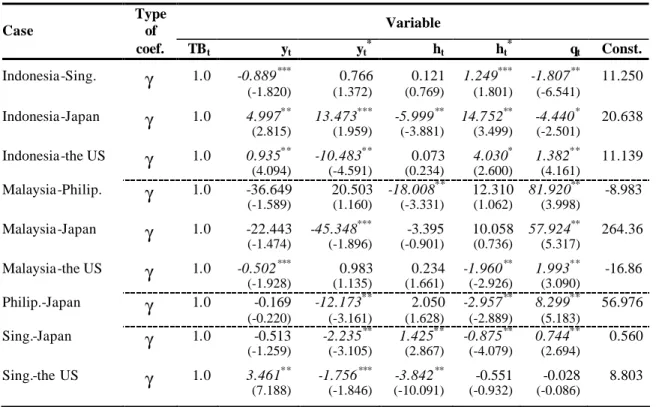
1.4.1 The long run relationship
Since the results of Johansen cointegration test show various numbers of cointegrating vectors in the bilateral cases which reject the null hypothesis, this suggests that the long run relationship is not unique. With respect to that, following Singh (2004), we decide to use the first cointegrating vector as the most likely vector in our not unique long run analysis due to it provides the maximal eigenvalue statistics in the test10. So, hereafter we consistently hold the idea when applying Johansen cointegration test.
In Table 6, the estimated coefficients of the first cointegrating vector (γ ) are normalized with respect to the coefficient of the Ln TB. Among all of bilateral cases which are reported, only the case of Indonesia-Singapore and Indonesia-Japan indicate an expected positive long run relationship between the real exchange rate (q) and the real bilateral trade balance (TB). With a long run elasticity of 1.81 and 4.44, respectively, they provide strong empirical support to the theoretically predicted real depreciation improves the trade balance in the long run. Marshall- Lerner condition holds in those bilateral cases. On the contrary, for other bilateral cases, this paper fails to find such a rela tionship. However, the case of Singapore-the US still shows an expected positive sign though it is statistically insignificant.
10