Ph.D. PROGRAM IN EARTH SCIENCES
XXXII CICLE
Integration of object-oriented modelling and geomorphometric
methodologies for the analysis of landslide systems
SSD GEO/05
Ph.D. Student
Mario Valiante
Tutor
Professor Francesca Bozzano
Co-Tutors
Professor Marta Della Seta
Index
Extended Abstract... i
1 Introduction ... 1
2 Theoretical background ... 4
2.1 Object-oriented data modelling ... 4
2.1.1 The object-oriented paradigm ... 4
2.1.2 Object-oriented databases ... 5
2.1.3 Object-oriented modelling for geospatial data ... 6
2.1.4 Hierarchy ... 7
2.2 Spatio-temporal data analysis ... 7
2.2.1 Topological models ... 8
2.2.2 Temporal models ...10
3 Object-oriented model for landslides ...11
3.1 Landslide classes (Focal level) ...11
3.2 Landslide complex classes (level +1) ...13
3.3 Landslide system class (level +2) ...15
3.4 Landslide component classes (level -1) ...15
3.5 Temporal characterization and vertical relations...16
4 Methods ...18
4.1 Top-Down approach ...18
4.1.1 Topographic Position Index ...18
4.1.2 Slope-Area plots ...21
4.1.3 TPI and S-A plots integration...22
4.2 Bottom-Up approach ...23
4.2.1 Landslides inventory and landslide maps ...23
4.2.2 Database design ...24
4.2.3 Reference hillslope ...28
4.3 Top-Down and Bottom-Up comparison ...30
5 Case studies ...32
5.1 Corniolo – Poggio Baldi ...32
5.1.1 Geological and geomorphological settings ...32
5.1.2 The Poggio Baldi landslides ...34
5.1.5 Approaches comparison ...43
5.2 Mt. Pruno – Roscigno ...45
5.2.1 Geological and geomorphological settings ...45
5.2.2 The Old Roscigno town ...47
5.2.3 Top-Down approach ...48
5.2.4 Bottom-Up approach ...50
5.2.5 Approaches comparison ...54
5.3 Rocca di Sciara ...55
5.3.1 Geological and geomorphological settings ...55
5.3.2 The 2015 Scillato landslide ...57
5.3.3 Top-Down approach ...58
5.3.4 Bottom-Up approach ...61
5.3.5 Approaches comparison ...66
6 Discussions ...68
6.1 The object-oriented model and its database implementation ...68
6.2 Top-Down vs Bottom-Up ...68
6.3 The reference hillslope ...70
7 Future developments ...71
8 Conclusions ...73
9 References ...75
Appendix ...88
Topographic Position Index (TPI) plugin for Grass GIS ...88
Extended Abstract
The main objective of my PhD research is to develop an object-oriented, hierarchical and multi-scale geomorphological approach to studying “landslide systems” meaning sets of landslides of different type evolving on the long-term with mutual interaction (sensu Guida et al. 1988, 1995; Coico et al. 2013; Valiante et al. 2016). The proposed approaches aim: 1) to improve the existing or new inventories, defining an object capable of storing both spatial and temporal relations between landslides in a single dataset, avoiding physical data fragmentation and logic inconsistency; 2) to build a robust conceptual model for the practical management of complex arrangements of landslides and their evolution.
This work also aims to contribute to the overall theme of landslide hazard assessment and mitigation, focusing on those cases where complex spatio-temporal arrangements of landslides interacts with engineering structures or infrastructures, for better understanding and quantify the interactions at various spatio-temporal scales between engineering works and natural processes. The research has been conducted following three main strategies: 1) a “Top-Down approach” based on morphometric analyses on Digital Elevation Models (DEMs) to find whether a portion of landscape shows a set of “topographic signatures” ascribable to landslide systems; 2) a “Bottom-Up approach” based on the reconstruction of the landslide system through field activities starting from any of the landslides composing the system itself; 3) comparison of the above strategies using a training-target approach on selected case studies significant for different Italian landscapes.
The “Top-Down” approach is based on the application of morphometric techniques using Digital Elevation Models, such as Topographic Position Index (TPI) (Weiss 2001; Paron and Vargas 2007; De Reu et al. 2013), useful for the semi-quantitative delineation of main landforms, and Slope – Area Plots (Montgomery and Foufoula-Georgiou 1993; Booth et al. 2013; Tseng et al. 2015), exploited for the estimation of the erosional processes type acting on the slopes, and extended also to gravity-driven processes. Basically, the graphical plot of the topographic steepness as function of the drainage area can be subdivided in four main plot regions or curve segments, each one representing a dominant geomorphic process: I) hillslopes; II) hillslope-to-valley transition; III) debris flow dominated channels or landslides driven channels; IV) alluvial channels.
The “Bottom-Up” approach follows the GmIS_UniSA method proposed in Dramis et al. 2011. In the first steps data collected from field activities were stored referring to a symbol-based representation (SGN 1994; APAT 2007; ISPRA 2018) similarly to what has been done by many authors (Gustavsson et al. 2006; Devoto et al. 2012; Miccadei et al. 2012; Del Monte et al. 2016 among the others), in the next steps the original data is extended from the symbol-based to a full-coverage representation. The latter is then reclassified using the proposed object-oriented data model.
Such object-oriented data model is based on the assumption that any entity can be represented by exactly one object regardless of its complexity or inner structure (Egenhofer and Frank 1992). Complexity is then handled through the classification process: a real-world feature and its behaviour is described and encapsulated in a class definition, then any operation of simplification or generalization can be performed defining a set of sub-classes and super-classes. Any feature
the description of a feature and its behaviour while an object is the feature itself (Atkinson et al. 1990; Chaudhri 1993; Kösters et al. 1997).
The described classification process results in a set of classes linked by parent-child relationship (generalized and specialized classes) and sibling relations (classes sharing a common super-class) in a hierarchical structure. Hierarchies are usually exploited to model, and therefore better handling complexity of natural systems; in this perspective a hierarchy is defined as a multi-level or layered system where each level can be decomposed in a number of interrelated subsystems until a non-decomposable elementary subsystem is defined (Simon 1962; Odum and Barrett 2005; Wu 2013). Depending on the objectives of a particular study or analysis, the hierarchical level closer to the study object is called focal level or level 0 which sets the starting point for decompositions (levels -x) or generalizations (levels +-x) (Wu 1999).
Applying the previous concepts, the basic landslide inventory is built by means of usual techniques, such as field survey, remote sensing, desk studies, etc., then an object-oriented hierarchical model is applied resulting in a hierarchical classification of landslides. The focal level is set at the input inventory containing individual landslides as one object differentiated by type of movement. The proposed model assumes that a “functional interaction” (i.e. dynamic interaction) exists if the condition of spatial and temporal overlap between landslides is verified. This assumption can be evaluated through the integration of two topological models. The Dimensional Extended nine-Intersection Model (DE-9IM) (Egenhofer and Herring 1990a, b; Egenhofer and Franzosa 1991; Clementini et al. 1994) and the Region Connection Calculus (RCC8) (Randell et al. 1992; Cohn et al. 1997). Starting from the focal level, 2 levels of generalization are defined based on the topological relation between landslides: i) if two or more landslides of the same type have a 2-dimensional relation between their interior portion, they can be simplified in a landslide complex object having the same type of movement as the input features; ii) if two or more landslide complexes have a 2-dimensional relation between their interior portion or with the interior of another landslide which is not part of the input complex, they can be simplified in a landslide system object. A level of decomposition has been also implemented describing landslide components.
Once derived a landslide system, it is useful to define its Reference Hillslope, meaning the minimal portion of territory in which it is likely to evolve. To address this task Surface Networks can be a valid technique in order to objectively define the minimal portion of the topographic surface in which a gravitational process can develop and evolve. The extraction of Surface Networks from DEMs (Pfaltz 1976; Wolf 1991; Schneider 2003; Rana 2004) is based on the detection of the characteristic features of a surface called critical elements, such as critical points (local minima, local maxima and local saddles) and critical lines (ridgelines, connecting peak and passes, and courselines, connecting pits and saddles). This data structure has been exploited to decrease complexity of topography representing just its “mathematical skeleton” (Guilbert et al. 2016). In order to test these methodologies, three italian case studies have been selected choosing sites with different geological settings and thus landsliding style. The choice of the study areas has been made also picking landslide recently reactivated with a great impact on anthropic activities. The selected case studies are:
· Roscigno (SA) on the south-western slopes of Mt. Pruno;
· North-eastern slope of the Rocca di Sciara relief in the valley of the Northern Imera river, close to Scillato village (PA).
The Corniolo – Poggio Baldi case study has been selected for the last reactivation of the Poggio Baldi landslide in March 2010. The movement developed as a rock-wedge slide evolving in a flow-like movement that produced the damming of the Bidente river and the formation of the Corniolo Lake, which is partially still present today. The main geological settings of the area are made of a sandstone-marly flysch with a dip-slope attitude.
The case of Roscigno refers the history of the abandoned “Old Roscigno” rural village. This ghost town has been transferred from about sixty years due to landsliding activity and is nowadays part of the Cilento UNESCO - Global Geopark. The village was built on the south-western slope of Mt. Pruno, mainly composed of terrigenous deposits such as calcarenitic-marly flysch, tectonically overlapping a clayey-marly flysch. The main movement affecting the slope is a deep-seated rock slope deformation, on top of which several shallow landslides developed, such as rotational slides and mud flows.
The Rocca di Sciara case study has been chosen for the last reactivation of the lower portion of the slope in April 2015. The event caused severe damages to the road network, also involving the Palermo – Catania highway leading to the failure of the Imera viaduct. The geological settings of the slope are made of a dip-slope bedding heterogenous sequence of limestone megabreccias and thick-bedded calcarenites, thin-thick-bedded or laminated calcilutites and clayey flysch.
During these three years of research, several survey activities have been performed in order to reconstruct the geological and geomorphological setting of the case studies. All these activities were supported by the object-oriented perspective defined before, allowing objects definition and description directly on the field.
Both the “Top-Down” and the “Bottom-Up” strategies have been applied to the case studies. As for the first strategy, the contributing area reclassification shows mainly the hypothetical landslide-related channel as linear features, while the TPI reclassification highlights concave morphologies that can be related to landslides components, such as detachment areas, trenches, counterslopes, and so on. Both these methods can be useful techniques to assess potential landslides affected areas for a better planning of further activities such as field surveys, which are the starting point of the second strategy. Following the data collection, by direct surveys, desk studies or remote sensing, all the information has been rearranged within the object-oriented logic perspective; then, the hierarchical model allows to derive higher rank units, such as landslide complexes and landslide systems. Based on these derived objects, through the integration of Surface Networks it is possible to define the so-called “Reference Hillslope” for each landscape object.
Every landslide is characterized not only by its attributes but also by it spatial and temporal relations with the other movements. Coupling this object-oriented hierarchical approach with a temporal characterization of landslide features in the form of “events”, semantically defined, it is possible to build an object-oriented and event-based database capable of storing both spatial and temporal
The Top-Down approach showed some limitation in the recognition of deep-seated movements, while the Bottom-Up approach allowed the automatic reconstruction of the landslide hierarchies starting from the landslide inventory. A landslide system built with an accurate spatio-temporal inventorying of landslides can be a tool for the fast retrieval of useful information such as “how many events affected a slope and how they developed, their magnitude and frequency and how they interacted”. All these data regarding the past and present activity of a slope are the assumption for understanding its most likely evolution, thus, to contribute to the formulation of reactivation scenarios. Moreover, the definition of the “reference hillslope” allow to objectively define the area/volume to be investigated starting from a reference object – a landslide, a landslide complex or a landslide system - , both for the planning of remediation and monitoring activities and as a starting point to search whether a landslide interacts with other geomorphic processes or anthropogenic activities.
1
Introduction
In the field of natural hazards, landslides are one of the most widespread and frequent occurrences, related both to natural and anthropic triggers, sometimes with catastrophic outcomes such as loss of lives (Evans et al. 2007; Cascini et al. 2008; Petley 2012; Barla and Paronuzzi 2013; Froude and Petley 2018). Landslides also often interfere with human activities, impacting on urban areas, various infrastructures such as roads, tunnels, bridges, pipelines and so on, and areas related to other socio-economic activities causing great economic losses (Alexander 1988; Fiorillo et al. 2001; Crosta et al. 2004; Evans and Bent 2004; Gattinoni et al. 2012; Genevois and Tecca 2013; Maiorano et al. 2014; Pankow et al. 2014; Schädler et al. 2015; Uzielli et al. 2015; Klose 2015; Bozzano et al. 2016; Smaavik and Heyerdahl 2016; Valiante et al. 2016; Bozzano et al. 2017; Esposito et al. 2017; Marinos et al. 2019 for example). In this framework, sometimes, structures or infrastructures are faced with complex arrangements of landslides rather than a single movement (Barredo et al. 2000; Borgatti et al. 2006; Corsini et al. 2006; Guida et al. 2006; Guerricchio et al. 2010; Di Martire et al. 2015; Schädler et al. 2015; Uzielli et al. 2015b; Bozzano et al. 2016; Lupiano et al. 2019). Such complexity can be related to different spatio-temporal arrangements of landslides: there can be a frequent occurrence of phenomena in a relatively small area (Haigh et al. 1993; Corbi et al. 1996; Crozier 2010a, b; Berti et al. 2013; Roback et al. 2018), or the spatial overlap of successive landslide events, like converging flow-like movements (Zuosheng et al. 1994; Cascini et al. 2008; Schädler et al. 2015), or relatively shallower phenomena developed over deep-seated movements (Guida et al. 1987; Guerricchio et al. 2000; Murillo-García et al. 2015), or partial mobilizations of previous landslides in nested structures (Lee et al. 2001), or various superimpositions of different landslide types (Stefanini 2004; Guida et al. 2006; Di Martire et al. 2015; Valiante et al. 2016) . Overlapping landslides derive from the temporal sequence of events and some authors already noticed that such cases need further attention and cannot be managed as a simple landslide (Corbi et al. 1999). Other authors also suggested the concept of path dependency for landslide susceptibility analysis, stating that pre-existing landslides could be a predisposing factor for future phenomena (Samia et al. 2017a, b). Besides spatial arrangements of landslides, even dealing with a single landslide implies to face its inner complexity, i.e. describe its components (Parise 1994, 2003; Fiorillo et al. 2001; Dai and Lee 2002; Niethammer et al. 2012; Dufresne et al. 2016; Morelli et al. 2018; Wang et al. 2018b; Catane et al. 2019). In this framework, when an active landslide considered in an engineering problem is part of a broader deformation/failure/flow context, define the reference area for remediation works or monitoring activities is quite a challenge, ideally it should be addressed taking into account the state of activity, hence frequency, of movements and their temporal evolution related to the temporal persistence of the geotechnical project object of the study.
Even in the cases where the object of the study is clear, being it a single landslide or a set of them, define the corresponding minimal portion of landscape to analyse is an open question. Sometimes geotechnical investigations or monitoring activities are planned and executed within the active landslide area or in its closer surroundings (Borgatti et al. 2006; Torreggiani 2009; Romeo et al. 2014; Abolmasov et al. 2015; Di Martire et al. 2015; Mazzanti et al. 2017), leaving out the geomorphological context in which the referenced phenomenon developed. Defining an objective “area of interest” starting from a well-known object may be an interesting task to address, in order to optimize
landscape units as a basis for landslides analysis is not an easy task as well. Various methods have been proposed defining landscape partitions with different methodologies, such as grid-cells, terrain units, unique-condition units, slope units and topographic units (Carrara et al. 1991; Guzzetti et al. 1999 and references therein; Alvioli et al. 2016). All of them have been exploited for landslide susceptibility analyses (Carrara et al. 1991; Aleotti and Chowdhury 1999; Chung-Jo and Fabbri 1999; Van Westen et al. 2003; Yesilnacar and Topal 2005; Piacentini et al. 2012; Budimir et al. 2015; Luo and Liu 2018; Reichenbach et al. 2018). They are not suitable for site-specific scale studies, as they are usually computed at smaller scales and do not consider pre-existing landslides in their definition. Existing inventories currently do not have the capability to store and retrieve such complexity in landslide arrangements, both because of the lack of a model describing spatio-temporal overlapping phenomena and because, most of the times, is not even possible to store or represent overlapping features within the same dataset as this is treated as a topological error (ESRI 2019). Despite this is extremely useful for various applications, such as administration boundaries or cadastral management, dealing with landslides, it is a crude limitation. Representing nested or overlapping landslides as a coverage of adjacent tiles produce a logic inconsistency between the topology of the data and the topology of the real-world features, as vertical relations between landslide events such as under-over, contained-contains, overlapping-overlapped, are not preserved causing a loss of information. Besides, current approaches in multi-temporal landslide inventories are usually based on the snapshot or “time-slices” model (Dragicévić 2004; Guzzetti 2006; Samia et al. 2017a), representing with different datasets the landslide inventory at a specific time or landslide events occurred in a specific time frame. Having multiple datasets for representing multitemporal information results in data fragmentation and a poorly management of temporal relations.
In order to describe spatial and temporal arrangements of landslides Guida et al. 1988 introduced the concept of landslides system as “a set of complex landslides (sensu Varnes 1978; Cruden and Varnes 1996) ascribable to a common initial deformation which, on long-term evolution, develops into differentiated morphotypes referring to type of movement, age and state of activity”. The authors further differentiated the description of landslides associations based on movement types and state of activity (Guida et al. 1995) and since then, such terminology has been rarely used for the description of landsliding phenomena in southern Italy (Guida et al. 2006; Coico 2010; Sinistra Sele River Basin Authority 2012; Coico et al. 2013; Valiante et al. 2016).
Starting from the overall topic of the definition of the relations between complex arrangements of landslides and engineering works, this research aims to: i) define a conceptual model, based on the concept of “landslide system”, for the description of associations of landslides and their spatial and temporal relations; ii) implement such a model in a database structure capable of storing both spatial and temporal information in a single dataset, avoiding physical fragmentation and logic inconsintency of the data, allowing to quickly retrieve information about the number of interacting phenomena, their temporal occurrence, hence the slope evolution, their spatial relations and so on; iii) define an objective methodology to bound the minimal area to be attentioned for a landslide or a set of landslides.
The model has been developed defining an original object-oriented and hierarchical classification for landslides. In this hierarchy, landslides are preliminarly defined at the focal level and two levels of aggregation based on topological relations describe various association of landslides. After, just
one level of decomposition containing landslide components was defined, leaving a second one (landslide element) for further geospatial, topological and mereo-logical researches.
The object-oriented data model has been chosen as optimal knowledge reasoning and representation of the geospatial domain of interest, because of its intrinsic hierarchical structure, its flexibility in the classification procedures, adapting to any natural system, and the capability to define procedures (called methods or functions) to dynamically access and manipulate classes attributes reducing the volume of information needed to be actually stored (Egenhofer and Frank 1987; Worboys et al. 1990; Worboys 1994; Kösters et al. 1996). This model is not a new landslide classification technique as it relies on existing classifications for movement types (Varnes 1978; Cruden and Varnes 1996; Hungr et al. 2014), but it is intended for the description of landslide associations, their spatial and temporal relations and as a tool to build, update and manage landslide inventories.
2
Theoretical background
2.1
Object-oriented data modelling
In the field of geosciences, words as “object-oriented” or “object-based” usually refer to the well-known technique of the Object-Based Image Analysis (OBIA). This practice is based on the classification of raster datasets mainly by clustering pixels sharing common properties defining vector polygons called “objects”, which can be further decomposed or aggregated following user-defined rules (Hay and Castilla 2008; Blaschke et al. 2014; Louw and van Niekerk 2019). This segmentation procedure can be applied on any raster dataset for several purposes such as on Digital Elevation Models (DEM) and their derivatives (slope, curvature, hydrology, etc…) for landforms recognition (Drǎguţ and Blaschke 2006; Eisank et al. 2011; Guida et al. 2012; Barzani and Salleh 2016), as well as on multispectral or panchromatic remote sensing imagery for land-use/cover analysis (Zhou et al. 2009; Li et al. 2014; Wang et al. 2018a). Efforts have been made also in the automatic recognition of landslides using OBIA both on DEMs and various remote sensing products (Fernández et al. 2008; Van Den Eeckhaut et al. 2012; Feizizadeh and Blaschke 2013; Moosavi et al. 2014; Mezaal and Pradhan 2018). The common foundation of all the OBIA techniques is that every image (digital domain) depict real-word features (concept domain), thus every “image object” derived through OBIA should correspond to a “geographic (geomorphological) object” (Castilla and Hay 2008; Eisank et al. 2011). However, all these concepts are borrowed from the original object-oriented paradigm, OBIA is just one of its applications.
2.1.1 The object-oriented paradigm
Object-orientation concepts were developed in the ‘60s as structures for programming languages in order to overcome existing limitations. Then-existing simulation languages, based on procedural standards as a set of instructions, were not sufficient to model real-world systems (Holmevik 1994; Kindler and Krivy 2011). The need to develop a programming language containing both a system description and the functions describing its processes, led to the invention of Simula, considered the first full-fledged object-oriented programming language (Dahl and Nygaard 1968; Dahl 2002). Most of the languages used nowadays for scientific applications are object-oriented, the most relevant are C++, Java, Python and partially R and MATLAB. According to Lewis and Loftus (2015) and Phillips (2018), the key concepts or main features of any object-oriented language are:
· Abstraction: features can be described through a classification, i.e. any feature is modelled with a class definition containing both its description and variables (attributes) and the procedures or functions available for that class (methods). Any instance (practical example) of that specific class is called object. Relations between classes are modelled through generalization, association and aggregation;
· Encapsulation: variables and functions definition inside a class allow final users to manipulate objects through methods without interfering with the original properties of the class itself (data hiding);
· Inheritance: classes can contain sub-classes which share their super-class attributes and methods;
· Polymorphism: different object types have their own different implementation of the same function or method.
2.1.2 Object-oriented databases
With the spreading of object-oriented programming languages, users started to think whether Database Management Systems (DBMS) could also benefit of the object-oriented paradigm features. The well-established Relational model (Codd 1970) (RDBMS) proved some limitations such as lack of complex data types, data structures limited to the table format, atomic values, etc. (Chaudhri 1993; Ghongade and Pursani 2014; Aziz et al. 2018).
According to The Object-Oriented Database System Manifesto (Atkinson et al. 1990), a DBMS to be defined as such, must ensure at least:
· Support for complex objects: tuples, lists, arrays, multimedia data types, etc., as well a set of operators to handle them;
· Object identity: any object exists regarding of its values, meaning that any values alteration (updates) do not compromise object persistence. This can be extremely useful for referencing and assignment operations;
· Encapsulation: as in the original concept, both the data describing a model and the procedures available for that model are stored within the database;
· Classification: any object is described by a set of attributes and can be manipulated with a set of functions both declared by a class definition;
· Class hierarchies: subclass definitions allow to share attributes and methods among classes related by parent-child relation;
· Overriding: this is a derivation of the polymorphism concept. Different classes can have the same names for attributes or methods, but the underlying behaviour is different;
· Extensibility: users can add their custom classes, data types and functions;
· Persistence: obviously, as required for any DBMS, data must survive the execution of the process defining them to be reused in another process;
· Secondary storage management: the DBMS should be able to manage any kind of support for the storage of data;
· Concurrency: data should be accessible by different users at the same time; · Recovery: data integrity should be ensured in any case of system failure; · Ad Hoc Query Facility: data should be queryable.
Even if Object-Oriented Database Management Systems (OODBMS) have been developed and existed in the last 20 years, they struggled to be a valid competitor for RDBMS. This is due mainly to the lack of standards, in fact RDBMS can rely on a strong mathematical basis and on a unified Structured Query Language (SQL) while OOBDMS strongly depends on the language they are conceived (Aziz et al. 2018). However, different DBMS, though being notoriously based on the Relational model, started to implement several features of the Object-Oriented model in the last years. Such hybrids have been defined Object-Relational Database Management Systems (ORDBMS) ant two renowned examples are the open-source PostgreSQL and the commercial Oracle DB (Oracle® 2019; The PostgreSQL GDG 2019).
Figure 1 – The relational model (a) compared to the object-oriented model (b)
2.1.3 Object-oriented modelling for geospatial data
OODBMS have been widely acknowledged as the optimal structure for the storage and manipulation of geographical information (Löwner 2013). Egenhofer and Frank (1987) firstly proposed an object-oriented model for the manipulation of spatial information based on the abstraction concepts of classification, generalization and aggregation, introducing a hierarchical structure with single or multiple inheritance of attributes and methods. Following their pioneering work, a series of concepts and structures have been proposed. To better model interactions among the defined classes, Worboys et al. (1990) introduced functional relationships between object as links describing their mutual connections. Later they characterize geo-objects having a four-dimensional structure (Worboys 1994):
· Spatial dimension, which defines geometrical and topological properties; · Temporal dimension, where their persistence in time and evolution is stored; · Graphical dimension, storing properties regarding the graphical representation; · Textual-numerical dimension, storing attributes and data.
Upon these bases, several data structures have been proposed both for general-purposes spatial databases (Egenhofer and Frank 1992; Kösters et al. 1996; Fonseca and Egenhofer 1999; Borges et al. 2001; Khaddaj et al. 2005) and specialised data, such as census/administrative units (Worboys et al. 1990), topographic information (Shahrabi and Kainz 1993), archaeology (Tschan 1999; Holt 2007) and city planning (Gröger et al. 2004). Moreover, different specialized applications have been developed based on object-oriented models (Câmara et al. 1996; Kiran Kumar et al. 1996; Kösters et al. 1997; Posada and Sol 2000; Holt 2007; Chen et al. 2012).
Abstraction mechanisms to describe a system are based on the assumption that any entity can be represented by exactly one object regardless of its complexity or inner structure using classification (Dittrich 1986). Complexity is modelled through generalization, association and aggregation (Egenhofer and Frank 1992). Generalization groups several classes of objects with common operations into a more general super-class, and it is described by the relations is-a or can-be-a, the inverse process is specialization; association relates two or more independent objects which can have an identity as a group, it is described by the relations member-of or a-set-of; aggregation relates an
entity with its components and is described by the relations part-of or consists-of, the inverse process is decomposition (Figure 2).
Figure 2 – Generalization (a), association (b) and aggregation (c). (modified from Hegenhofer & Frank, 1992)
2.1.4 Hierarchy
As described before, object-oriented methods strongly rely on relationships among classes. These relations can be such as generalization-specialization, aggregation-decomposition or association: all these connections define a hierarchical structure.
In a hierarchical structure, classes and sub-classes are related by parent-child relationship, while classes sharing a common super-class are called siblings (Tsichritzis and Lochovsky 1976; Singh et al. 1997; Glover et al. 2002; Malinowski and Zimányi 2004). A hierarchy is defined as a multi-layered system, where each level can be decomposed until a non-decomposable level is defined (Simon 1962; Odum and Barrett 2005; Wu 2013). While the object-oriented classification defines specific relationships among classes, hierarchical levels are a relative structure and depend on the purpose to which they are applied. Based on the objective of an analysis, the centre of the hierarchy (Focal level) can be any object of interest, and its parents define levels of generalization or aggregation (levels +x), while its children define levels of specialization or decomposition (levels -x) (Wu 1999, 2013) (Figure 3).
Figure 3 - Hierarchical structure (modified from Wu, 2013)
2.2
Spatio-temporal data analysis
Typical queries and operations on geographical objects often are based on their spatial properties and temporal attributes. A major benefit of spatial databases over general-purpose databases is indeed the integration of common functions capable of reading and manipulating the basic spatial characteristic of an object in order to retrieve more complex spatial relationships. Such capabilities are the foundation of all the modern Geographic Information Systems (GIS) (Heywood et al. 2006).
Spatial relationships can be classified in three main categories (Egenhofer and Herring 1990a): · Geometric relationships: anything that can be measured within a referenced system, such as
distances, directions and angles, areas, volumes, etc.
· Spatial order relationships: regarding the objects ordering in a referenced space. These properties are usually dualistic and common examples are in front – behind or above – beneath; · Topological relationships: describing the relative arrangements of objects in space. These properties are usually invariant under common transformations or distortions such as translation, scaling, rotating, stretching, etc.
Temporal queries require the modelling and storage of temporal information. Time could be expressed as a point or as an interval where time points represent exact moments and time intervals represent any time span. However, both these two definitions can be generalized in time intervals, as time points are a relative concept and depend on the time scale in which they are referred (Allen 1983; Nebel and Bürckert 1995; Van Beek and Manchak 1996). Relations among time intervals are defined in Allen 1983, describing their relative position in the time dimension (Figure 4). Temporal Geographic Information Systems (T-GIS) are defined as GIS capable of storing and manipulating temporal information in order to perform spatio-temporal queries (Yuan 2008).
Figure 4 - Allen's temporal predicates (modified from Nebel & Bürckert, 1995)
2.2.1 Topological models
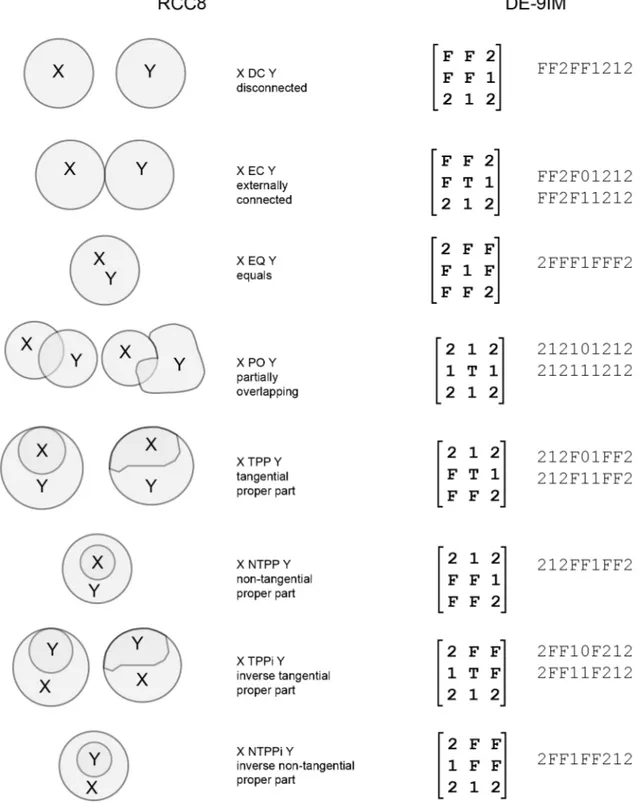
To describe spatial relations between objects, two topological models for spatial reasoning have been exploited in this work: the Dimensionally Extended nine-Intersection Model (DE-9IM) (Egenhofer and Herring 1990a, b; Egenhofer and Franzosa 1991; Clementini et al. 1994) and the Region Connection Calculus (RCC) (Randell et al. 1992; Cohn et al. 1997). The DE-9IM is a topological model used to describe the spatial relations of two geometries (points, lines, polygons) in two dimensions. The basic assumption for this model is that every object in the R2 space has an interior ( ( ) = ), a boundary ( ( ) = ) and an exterior ( ( ) = ) and the spatial relation of two geometries is evaluated in the form of a 3x3 intersection matrix with the form:
9 ( , ) =
dim ( ∩ ) dim ( ∩ ) dim ( ∩ ) dim ( ∩ ) dim ( ∩ ) dim ( ∩ ) dim ( ∩ ) dim ( ∩ ) dim ( ∩ )
where dim is the maximum number of dimensions of the intersection of the interior, boundary, and exterior of geometries a and b (dim(point) = 0, dim(line) = 1, dim(polygon) = 2). These values can be expressed as boolean values where FALSE means non-intersection and TRUE any other value. The resulting matrix can be also expressed as a 9 characters alphanumeric string. RCC describes regions by their possible relations to each other. RCC8 consists of 8 basic relations that are possible between two regions. Integrating the two models, RCC8 relation can be converted in 12 DE-9IM matrices and thus in 12 alphanumeric strings which can bel implemented in a database dictionary (Figure 5).
2.2.2 Temporal models
Time can be handled in different ways in GIS, thus in databases. Two recurrent models are the snapshot model and the event-based model. In a snapshot model, each dataset represent the state of a system in a precise time frame, it could be considered as a photography of a system’s state in a specific instant (Peuquet and Duan 1995; Dragicévić 2004; Gutierrez et al. 2007). In event-based approaches, objects within a dataset are characterized with temporal attributes describing their time persistence (Peuquet and Duan 1995; Worboys and Hornsby 2004). Referring to landslides, an event can be described as a set of landslides mobilized by the same trigger (Napolitano et al. 2018) or by domino-effect (Martino 2017). The main difference between these two models is that in the snapshot model the temporal characterization is assigned to the whole dataset, while in the event-based approach, objects within the dataset have their own temporal characterization. Using an event-based approach reduce data fragmentation, allowing to store all the information within one dataset and, at the same time, reduce data redundancy which reflect a reduction in data volume.
3
Object-oriented model for landslides
The object-oriented model developed in this research relies on terminologies and concepts previously introduced for the study of peculiar spatial arrangements of landslide phenomena. Guida et al. 1988 introduced the concept of “landslide system” as “a set of complex landslides (- a slope movement that involves a combination of one or more of the principal type of movements - sensu Varnes 1978; Cruden and Varnes 1996) ascribable to a common initial deformation which, on long-term evolution, develops into differentiated morphotypes referring to type of movement, age and state of activity”. Later on, they defined a more detailed classification for interconnected landslides based on the comparison of their type, age and state of activity (Guida et al. 1995):
· Landslide association – having same type of movement, same age and same state of activity; · Landslide group – having same type of movement, same age and different state of activity; · Landslide family – having same type of movement, different age and different state of
activity;
· Landslide system – having different type of movement, different age and different state of activity.
Following the hierarchical and multi-scalar model for geomorphological mapping described in Dramis et al. 2011, the previous classification has been simplified. The focal level (level 0) of the hierarchy is composed by the landslides themselves while two levels of generalization describe sets of landslides: i) landslide complexes result from the aggregation of landslide with the same type of movement spatially connected (level +1); ii) landslide systems are defined as a set of landslides of any type spatially connected (level +2). A level of decomposition stores landslide components (level -1). In this work the defined hierarchical and multi-scale classification has been structured in an object-oriented model suitable for database design and rules for the aggregation of landslides based on topological relations have been defined. An event-based approach has been also implemented in order to store and manipulate the temporal characterization of landslides.
3.1
Landslide classes (Focal level)
In this level landslides are classified referring to the updated classification of Hungr et al. 2014 (Figure 7). Classes are defined primarily considering the main type of movement, then the involved material. The original 32 types (48, if movements involving soils and rock-ice are distinguished) proposed by the authors are grouped into 21 landslide classes. This merging operation has the only purpose to simplify the aggregation procedure for the next level of generalization (§ 3.2) and does not intend to generalize the original classification, in fact, every class here defined as two movement type attributes, in which types are picked from the original 48 types discussed in Hungr et al. 2014 (§ 4.2.2). The 21 classes that have been identified are:
1. Rock fall class – class containing rock falls;
2. Soil fall class – includes granular materials falls, such as boulder falls, debris falls and silt falls;
3. Rock topple class – includes topple phenomena involving rock materials, such as rock block topples and rock flexural topples;
5. Rock rotational slide class – contains rock slides with a main rotational movement component;
6. Rock planar slide class – contains rock slides on a planar surface; 7. Rock wedge slide class – rock slides on a wedge-like surface; 8. Rock compound slide class – contains rock compound slides; 9. Rock irregular slide class – containing rock irregular slides;
10. Soil rotational slide class – includes clay rotational slides and silt rotational slides;
11. Soil planar slide class – contains clay planar slides, silt planar slides, gravel slides, sand slides and debris slides;
12. Soil compound slides class – class containing clay compound slides and silt compound slides; 13. Rock slope spread class – contains rock slope spreads;
14. Granular soil spread class – includes sand liquefaction spreads and silt liquefaction spreads; 15. Cohesive soil spread class – class containing sensitive clay spreads;
16. Rock avalanche class – class containing rock avalanches;
17. Soil dry flow class – includes sand dry flows, silt dry flows and debris dry flows;
18. Granular soil wet flow class – contains sand flowslides, silt flowslides, debris flowslides, debris flows, debris floods and debris avalanches;
19. Cohesive soil wet flow class – includes sensitive clay flowslides, mud flows, earthflows and peat flows;
20. Deep-seated slope deformation class – contains mountain slope deformations and rock slope deformations;
21. Shallow slope deformations class – includes soil creep processes and solifluctions.
Currently, all these classes share the same set of basic attributes, which are described in the next chapter where the database design is discussed. Methods (functions) developed so far are also shared among these classes and mainly deal with spatial and temporal properties of the objects:
· Events – retrieve the recorded events involving the referenced landslide;
· First-event – retrieve the first recorded event involving the referenced landslide; · Last-event – retrieve the last recorded event involving the referenced landslide;
· Siblings-complex – retrieve all the landslides forming the landslide complex in which the referenced landslide is contained, spatial and temporal relations are specified;
· Siblings-system – retrieve all the landslides forming the landslide system in which the referenced landslide is contained, spatial and temporal relations are specified;
· Parent-complex – retrieve the landslide complex in which the reference landslide is contained;
· Parent-system – retrieve the landslide system in which the reference landslide is contained; · Components – retrieve the referenced landslide components.
Figure 7 - The revised Varnes classification for landslides (from Hung et al., 2014)
3.2
Landslide complex classes (level +1)
The definition of the landslide complex classes relies on the concept of functional interaction between objects (Worboys et al. 1990). To form a landslide complex object, referring to the DE-9IM topological model, a functional interaction is defined as a 2-dimensional topological relation between objects members of the same landslide class (§ 3.1). Based on the RCC8 model, two or more landslide objects are eligible for the aggregation in a landslide complex object if their topological relation is partially overlapping, tangential proper part, inverse tangential proper part, non-tangential proper part or inverse non-tangential proper part. The equals relation, even satisfying the functional interaction requirements is unrealistic (Figure 8). Landslide objects that do not share functional interaction with other landslide objects, are reported as “isolated landslides” and do not reach the aggregation phase (Figure 9a).
Having 21 landslide classes, the same amount of landslide complex classes is derived: 1. Rock fall complex class;
2. Soil fall complex class; 3. Rock topple complex class; 4. Soil topple complex class;
5. Rock rotational slide complex class; 6. Rock planar slide complex class;
8. Rock compound slide complex class; 9. Rock irregular slide complex class; 10. Soil rotational slide complex class; 11. Soil planar slide complex class; 12. Soil compound slides complex class; 13. Rock slope spread complex class; 14. Granular soil spread complex class; 15. Cohesive soil spread complex class; 16. Rock avalanche complex class; 17. Soil dry flow complex class;
18. Granular soil wet flow complex class; 19. Cohesive soil wet flow complex class;
20. Deep-seated slope deformation complex class; 21. Shallow slope deformations complex class.
As for the landslide classes, currently, all these classes share the same set of attributes and methods. Attributes will be discussed in the database design chapter (§ 4.2.2), while the defined methods are: · Events – retrieve the recorded events involving landslides contained in the reference
complex;
· First-event – retrieve the first recorded event for the reference complex; · Last-event – retrieve the last recorded event for the reference complex;
· Siblings – retrieve all the complexes forming the landslides system in which the reference complex is contained;
· Parent – retrieve the landslide system in which the complex is contained;
· Movement types – retrieve all the movement types contained in the reference complex; · Landslides – retrieve all the recorded landslides forming the reference complex.
3.3
Landslide system class (level +2)
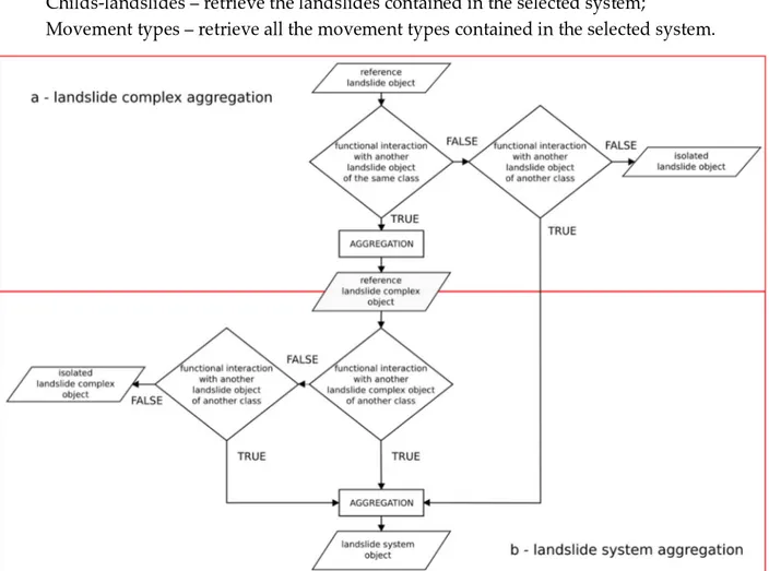
The landslide system class is built upon the aggregation of the previous declared classes. In this case the condition of functional interaction is defined as a 2-dimensional topological relation between two or more landslide complex objects or landslide objects of any type. In this case, landslides that do not form a complex can be aggregated in a system directly if they have a functional interaction with complexes or other landslides of different type. The topological relations that satisfy the functional interaction condition are the same as for the landslide complex classes. Landslide complex objects that do not share a functional interaction with other objects, as for landslide objects, are reported as “isolated landslide complex” (Figure 9b).
Methods available so far for this class are:
· Events – retrieve the recorded events involving the landslides contained in the selected system;
· First-event – retrieve the first recorded event for the selected system; · Last-event – retrieve the last recorded event for the selected system;
· Childs-complex – retrieve the landslide complexes contained in the selected system; · Childs-landslides – retrieve the landslides contained in the selected system;
· Movement types – retrieve all the movement types contained in the selected system.
Figure 9 - Logical model for the aggregation of landslide complex objects and landslide systems objects
3.4
Landslide component classes (level -1)
be considered for a further level of detail (level -2) but are not included in this work. Moreover, the implementation has been limited at the actual classes needed for the training sites.
Referring for example to the rock rotational slide class, the sub-classes defined are: · RRS detachment area class – containing detachment areas;
· RRS body class – containing rock rotational slides accumulation areas.
3.5
Temporal characterization and vertical relations
Every landslide object has attached temporal attributes for the time of occurrence which define an event. The relationship between landslides and events is many-to-one, meaning that one landslide object corresponds to a single event while one event can contain multiple landslide objects. Time of occurrence can be expressed as an exact value, when the date of occurrence is known, or as a range, when the exact time of occurrence is unknown, but a time interval can be deduced. For landslides contained in the same time interval a relative chronology can be implemented, based on field observations, remote sensing data analysis or any other mean.
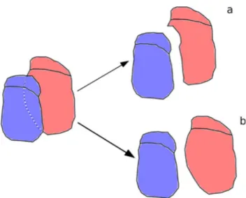
Temporal characterization of landslides is crucial for the correct management of vertical relationships. In this framework, vertical relationship means both spatial sorting of the type under – over and temporal sorting of the type older - younger. As for the law of superimposition, older objects lie under younger objects while younger objects lie over older objects. In particular cases where an older object is entirely mobilized by a deeper, younger object (tangential proper part or non-tangential proper part topological relations), the older object, even being physically over the younger object, loose its “status” of landslide object and became part of the new landslide object debris. Within the temporal dataset it will be displayed under the younger object, being older. In the case of several overlapping phenomena within the same event, an overlap index is introduced as secondary sorting parameter.
For better space-temporal data handling, basic topological relations have been integrated with temporal relationships. Based on the 8 relationships of the RCC model and Allen’s paradigms, referring to the object “A” and the object “B”, their topological relationship may vary whether A is younger than B or vice-versa (Figure 10):
· o → ∧ o → ∧ · ⋁ o → ∧ o → ∧ · ∨ o → ∧ o → ∧
The Equals relationship, as mentioned before, is not considered, while the Disconnected and the Externally Connected relationships are not affected by the temporal statement as their vertical sorting is invariant.
4
Methods
In order to test the proposed object-oriented hierarchical model, two main parallel strategies and a final comparative one have been developed and applied on three training sites in Italy.
In the Top-Down approach, morphometric analyses have been applied to investigate if complex arrangements of landslides, such as landslide systems, have a peculiar “topographic signature”. To this end, Slope-Area plots and Topographic Position Index have been used, the first for the topographic classification of slope processes, the latter for the definition of morphometric features ascribable to landslide processes. For all the raster elaborations, the open-source software Grass GIS©7.8.0 (current version) has been used, both for data storage and manipulation. For the computation of Topographic Position Index, a custom plugin written in python has been implemented inside Grass GIS©, the code can be found in the appendix.
At the same time, the Bottom-Up approach has been applied for the direct recognition of landslides, both from field activities and remote sensing data analysis. After landslide inventorying, the object-oriented hierarchical model has been applied and landslides hierarchies have been derived. Finally, results from the previous approaches have been compared to test the strength of the Top-Down approach for landslides identification.
4.1
Top-Down approach
4.1.1 Topographic Position IndexTopographic Position Index (TPI) has been defined as the integer difference between a point elevation ( ) and the mean elevation of its surrounding neighbourhood ( ̅) (Weiss 2001).
= (( − ̅) + 0,5)
So defined, TPI provides information about the relative position of a point in the landscape. Positive values mean that the elevation of the point is higher than the surrounding mean elevation, so the point is in a prominent-convex position, while negative values result from points having an elevation lower than that of their surroundings, so the point is in a depressed-concave position. Values near 0 represent points with an elevation about the same of the mean elevation of its neighbours, this is possible on flat areas or straight slopes (Figure 11).
On Digital Elevation Models (DEM) the algorithm compares the elevation of each cell with the mean elevation of the neighbourhood in which, usually, the reference cell is the central point. The neighbourhood needs to be defined in terms of shape and dimension. The most common neighbourhood geometries have been compared: circular, square and annulus (Jenness 2006; Tagil and Jenness 2008; De Reu et al. 2013). The annulus neighbourhood has a wider range of values but excludes data contained in the inner radius, while the square geometry has a short range of values. In this perspective, the circular neighbourhood has been selected as optimal both for completeness and resolution (Figure 12).
Figure 12 - Comparison of the resulting TPI values from different neighbourhood shapes, test on one of the case studies (§ 5.2) Once defined the neighbourhood geometry, the radius needs to be defined. Usually this step is an iterative procedure as the radius is set once the output meets the purpose of a particular study (Tagil & Jenness, 2008). To address the subjectivity in the choice of the radius, the analysis has been carried out on the aggregation of several outputs computed with an increasing value of radius following an exponential sequence of 2n cells, from 20 to 210, corresponding to a range of 5 m to 5120 m using a 5 m – resolution DEM. The various levels of TPI have been also standardized using the formula proposed in Weiss, 2001:
=
−
∗ 100 + 0,5
In this relation, mean and standard deviation parameters are derived from each raster dataset at every step. The result of this operation consists of two stacks of eleven raster datasets each, the first containing the effective TPI data and the last containing the standardized TPI data for every radius. Lastly, both the stacks have been aggregated by calculating mean and standard deviation (Figure 13). For the effective TPI values, datasets computed with larger neighbourhood have a major impact on the result because of their large values, while, for the standardized datasets, values are much more comparable as they are reduced at the same distribution size. In a morphometric perspective, this means that the mean of the effective values is more representative of the small-scale
raster datasets containing the mean values of both TPI and standardized TPI have been then reclassified using the 6 slope position scheme also suggested in Weiss, 2001, useful for basic landscape classification (De Reu et al. 2013; Kriticos et al. 2015; Gruber et al. 2017) (Figure 15).
Figure 13 - TPI datasets used for this study
Figure 14 - Comparison of the TPI values derived from the mean of the effective datasets and the mean of the standardized datasets, peaks of the TPIstd function are cut for readability; example profile from one of the case studies (§ 5.2)
Figure 15 - Slope positions
4.1.2 Slope-Area plots
Slope – Area Plots (Montgomery and Foufoula-Georgiou 1993; Booth et al. 2013; Tseng et al. 2015) have been exploited for the estimation of the erosional process types acting on the slopes, including also landslide phenomena. The purpose of this analysis is to detect the hypothetical landslide-related channels as a preliminary tool for landslides detection.
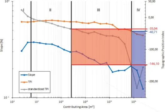
Basically, the graphical plot of the topographic steepness as function of the drainage area can be subdivided in four main regions or segments, each one representing a dominant geomorphic process: I) hillslopes; II) hillslope-to-valley transition; III) debris flow dominated channels or landslides driven channels; IV) alluvial channels (Figure 16a).
Slope and contributing area values have been plotted for each case study and domain thresholds have been defined analysing the slope derivative values (Vergari et al. 2019). Threshold for the I – II boundary has been set at the first zero value of the slope derivative, corresponding to the maximum value of the Slope – Area function; threshold between II and III domains has been set at the next zero of the derivative function which reflects an interruption in the steady decreasing trend of the II domain; the last threshold is marked by the last zero of the derivative values corresponding to the transition from fluctuating values to a steady decreasing trend in the slope function (Figure 16b).
4.1.3 TPI and S-A plots integration
For the recognition of landslide-related features an original comparison of TPI and slope values has been made as a new approach. Values from the mean TPI dataset and the mean standardized TPI dataset have been also plotted against the contributing area, defining a “TPI function” and a “Standardized TPI function”. Using thresholds derived from the S-A function, a range of values can be delimited on the Standardized TPI function corresponding to region III of the S-A plot defining a range of values that allow the reclassification of the mean standardized TPI raster into a set of morphometric features probably related to landslides. In the same way, a “fluvial domain” can be defined on the TPI function, corresponding to the IV region of the S-A plot. This new “fluvial region” obtained reclassifying the mean TPI raster has been used to filter features in the “landslides domain” obtained with the Standardized TPI function (Figure 17). The standardized TPI function has been chosen for landslide features identification as its values emphasize local morphological variations, while the effective TPI function is more suitable for the definition of the fluvial domain as its values reflect small-scale morphologies such as major valleys (Figure 18).
The range of standardized TPI values segmented with this approach is entirely composed of negative values. As negative TPI values correspond to concave morphologies, this analysis returns only concave features probably related to landsliding processes and not the entire landslide, convex portions of a landslide, such as bulgings and debris accumulations are not detected.
Figure 18 a c) mean values of the standardized TPI, continuous and reclassified using threshold shown in the previous figure; b -d) mean valued of the TPI values, continuous and reclassified; example from a case study (§ 5.3)
4.2
Bottom-Up approach
4.2.1 Landslides inventory and landslide maps
The basic landslides inventory has been built by means of field survey, remote sensing data analysis, such as aerial photographs and collecting data from previous existing inventories. Following the procedure proposed by Dramis et al. 2011 for general geomorphological mapping, inventoried features have been first stored with a symbol based approach (SGN 1994; APAT 2007; Gustavsson et al. 2008; Gustavsson and Kolstrup 2009; ISPRA 2018). Then, data have been processed in a GIS environment, converting symbols in proper landslide objects, producing a full coverage landslide map (Dramis et al. 2011; Guida et al. 2015) (Figure 20). In this full-coverage representation, the overlapping portions between landslides are preserved and not cut as usual, as they are crucial for the aggregation procedures (Figure 19). After these operations, data have been imported in the database designed following the proposed object-oriented model (§ 3).
Figure 19 - representing overlapping features a) as adjacent tiles cutting the overlapping portion, b) maintaining the overlapping portion ensuring correct topological relations
Figure 20 - GmIS-UniSA mapping model, the red square highlights the operations performed in the framework of this research (from Dramis et al., 2011)
4.2.2 Database design
The database used for this work is PostgreSQL© 11.0 with PostGIS© 2.5 extension (current versions). Database maintenance and manipulation is achieved using PgAdimn4 and the pgcli command line tool, while QGIS 3.4 LTR© is used for data query and visualization.
PostgreSQL© is an relational database management system (ORDBMS) and is not fully object-oriented, but a set of object-oriented features is already available:
· Inheritance – generalization and specialization are fully supported;
· Support for complex objects and extensibility – custom data types and functions can be declared;
· Overriding – the same function can have different behaviours based on the input arguments. Some other features are not natively implemented, but can be emulated with a few workarounds:
· Encapsulation and classification – these features can be emulated with custom data types for the attributes, and custom functions for methods;
· Aggregation – automatic aggregation based on class membership can be reproduced using PostgreSQL views and/or materialized views along with PostGIS aggregate functions like ST_Union or ST_Collect.
Lastly, object identity is not available as it is a concept strictly related to the object-oriented paradigm and as such, it is a feature only available in fully object-oriented languages and there is no way to implement such feature in a RDBMS. As for now, objects are stored as table records.
Based on the model described in § 1, the database has been structured into three main blocks: a dictionary block, a data block and a visualization block.
In the dictionary block, tables containing reference terminology are included. The main purpose of this data is to prevent errors during the process of data entry, therefore, to maintain data integrity. These tables are accessed through foreign key by the tables contained in the data block and by some of the dictionary tables themselves. The terminology contained in this block is about landslides (Hungr et al. 2014) and spatio-temporal topology semantics (Allen 1983; Egenhofer and Herring 1990b; Randell et al. 1992). The defined tables are:
· Landslides material types, containing reference information about landslides material; · Landslides movement types, containing reference information about landslides movement
type;
· Landslides types, containing reference terminology about landslide types, this table also refer to the material and movement type tables;
· Topological predicates, containing predicates for the RCC8 topological model and their corresponding matrixes for the DE9IM topological model;
· Temporal predicates, containing Allen’s predicates for temporal relationships;
· Spatio-temporal predicates, containing spatio-temporal predicated defined in § 3.5, this table also refer to the RCC8 and temporal table.
The data block is structured to contain the instances of the object-oriented model. Here, a table is defined for every class declared in the model (§ 1), meaning that the final result will be having 21 tables for landslide objects, 21 tables for landslide complex objects and one table for landslide systems. As for now, landslide tables are not further specialized as they share the same set of attributes:
· Landslide id, string type (‘LNS_nnn’) manual, contains the landslides id, this id is shared with reactivations of the same landslide;
· Event id, integer type mandatory, contains the event id for that landslide, these ids must be sequential, their ordering is the same of the temporal sequence of the events;
· Landslide event id, string type (‘LNS_nnn_nnn’) mandatory, this is the landslide unique id and derives from the combination of landslide id and event id and id used to distinguish between different reactivations of the same landslide, this is also the primary key of the table; · Overlap index, integer type mandatory, contains the overlap index for landslides of the same
event, default value is 0;
· Movement type 1, string type mandatory, contains the main type of movement of the landslide, refers to the movement types dictionary table;
· Movement type 2, string type optional, contains the secondary type of movement of the landslide, refers to the movement types dictionary table;
· Insert time, date type automatic, this field contains the time of data entry; · Date, date optional, this field contain the date when the landslide occurred;
· Date range start, date type optional, this field contains the starting date for the range of time in which the landslide occurred,
· Date range end, date type optional, this field contains the ending date for the range of time in which the landslide occurred.
· Geometry, geometry type mandatory, contains the geometry of the landslide.
Even though date, date range start and date range end are all optional fields, at least one of them is required for the correct temporal characterization of landslides. These fields are generic date types (YYYY-MM-DD), but if the only information available is a month or a year, they can be expressed as YYYY-MM-01 for months and YYYY-01-01 for years.
Landslide complex tables are materialized views derived from the aggregation of the landslide tables following the procedure described in § 3.2. These objects have not an exact temporal characterization as they can contain different landslides occurred at several times, but their vertical sorting is achieved computing the “mean event” from the aggregated landslides event ids, so that the most active complexes are ensured to be on top. Attributes for these tables are:
· Complex id, string type (‘CPX_nnn’) automatic, this is the landslide complex unique id and the primary key of the table;
· Mean event id, float type mandatory, this is the mean event id computed from the aggregation of the landslide tables;
· Geometry, geometry type automatic, contains the geometry of the landslide complex derived from the aggregation of the landslide geometries.
The landslide systems table, as for the previous tables, is a materialized view built upon the aggregation of the previous data. Attribute available for this table are:
· System id, string type (‘SYS_nnn’) automatic, this is the landslide system unique id and the primary key of the table,
· Geometry, geometry type automatic, contains the geometry of the system derived from the aggregation of the complexes and landslides geometries.
As for landslide complexes, systems have not an exact temporal characterization. Moreover, considering how they are built, for landslide systems vertical sorting is invariant as they do not overlap.
It is worth noting that attributes in this tables are essentials, meaning that the only data that is physically stored is about information that cannot be retrieved in any other way, for everything else, methods (functions) are used instead.
Landslide component table derive from the generalization of two main component groups, as far for the ones needed in this research:
· Detachments · Accumulations
These two categories branch themselves into the basic landslide components classes, as discussed in § 3.4. Attributes defined for these classes are:
· Landslides id, string type mandatory, contains the landslide unique id where the component belongs, referenced with the relative landslide table;
· Component id, string type (‘XXX_nnn’) automatic, contains the component id, it’s the primary key of the table;
· Geometry, geometry type mandatory, contains the geometry of the component.
In the visualization block, objects from the data block are re-arranged for the correct visualization. The vertical sorting is applied using the temporal characterization of landslides. This process only applies to components, landslides and complexes as systems, as for their definition, do not overlap, thus do not need vertical sorting (Figure 21).
Figure 21 - Database design for the proposed object-oriented model, acronyms for landslide tables and landslide complex tables refer to the classes defined in § 1
4.2.3 Reference hillslope
Once defined a landslide object or any other super-object, its interior could be described as the portion of landscape in which any observer is certain that that specific phenomenon (or several) is occurred or is occurring. On the other hand, its exterior should be the portion of landscape in which any observer is equally certain that the same phenomenon is not occurred or is not occurring. However, the latter statement could be not so true in the closer proximity of a landslide boundary, this area could be described as the portion of landscape in which there is no occurrence at the observation time but at the same time has the highest likelihood to be involved in a future reactivation. In this regard, referring to the egg-yolk model (Clementini 2004; Bittner and Stell 2008; De Felice et al. 2011), a landslide, or its generalizations, can be defined as a landform, or a complex or a system considering super-objects, with broad boundaries, with a core region and a vague or uncertain boundary (Cohn et al. 1997; Guilbert et al. 2016; Guilbert and Moulin 2017) (Figure 22).