A multi-robot system : from design to intelligent cooperation

(1)

UNIVERSITÀ DEGLI STUDI

ROMA

TRE

Scuola Dottorale in Ingegneria - Sezione Informatica e

Automazione

XXIII Ciclo

A multi-robot system: from

design to intelligent cooperation

Maurizio Di Rocco

A.A. 2010/2011

Tutor: Prof. Giovanni Ulivi

(2)

(3)

1. Reviewer: Achim J. Lilienthal

2. Reviewer: Paolo Robuffo Giordano

(4)

Maurizio Di Rocco

Scuola Dottorale in Ingegneria - Sezione Informatica e Automazione XXIII Ciclo

A thesis submitted for the degree of PhilosophiæDoctor (PhD)

(5)

Abstract

The proposed work aims at giving a contribution in the domain of multi robot systems. In the last years these architectures, thanks to their flexibility and robustness with respect to monolithic structures, have been deeply investigated in various applications. Looking at commercial platforms, one of the main limitations relies on the hard-ware configuration. In most of cases, the low-level control softhard-ware is not open source, compromising a detailed customization of the robot. This drawback can be partially overcome by the usage of plug-in boards which ease the use of a particular sensor. How-ever, whenever an application requires heterogeneous transducers, the management of several boards increases the computational burden of the CPU, the energy consumption and costs.

The first contribution of this thesis is the description of the prototyping of a multi robot platform. The robots, based on a dual layer architecture, have been designed to be low-cost and flexible in order to cope with several scenarios. The reduced di-mensions allow the units to execute experiments in small environments, like the ones typically available in a research laboratory, even interacting with commercial platforms like sensor networks.

Afterward, several experimental research activities are covered.

In the field of motion control, two techniques for the encircling problem, i.e. the task in which a set of robots rotates around a target, are presented. This toy problem is very appealing to the scientific community because it deals with a series of technological issues which involve communications, motion estimation and control design.

Also the data fusion, which is one of the most treated problem in robotics, has been taken into account. One of the traditional approaches resides on the Bayesian framework. This approach allows a straightforward combination of data gathered by several sensors. In this dissertation, such technique has been used in environmental

(6)

techniques can be used. In particular a focus on the Transferable Belief Model (TBM) is provided. Unlike the probabilistic formulation, the TBM is able to effectively repre-sent the concept of ignorance and contradiction, concepts which, for example, belong to the human kind of thinking. In this work a technique for the data fusion in a multi agent context is proposed. The theoretical results have been validated by extensive experiments concerning the cooperative topological map building.

Finally a lookup view about the integration between mobile and static sensor net-works (SN) is provided. One of the main issues for a static network is to know about the interdistances between nodes. In this work a localization algorithm, based on a modified Extended Kalman Filter, is showed. As for the previous topics, experimental results support the theoretical approach.

(7)

To every person who transparently and selflessly gave me the gift of his time,

(8)

This thesis represents the work of 3 years. During these years, I learned tons of things and I really would like to thank all of those people who helped me. First of all, I really would like to thank all of the students who worked in a passionate way: they gave me enthusiasm during the hours spent in the lab. A particular thanks goes to Giovanni and Enrico. Second, I really thank people who contributed to develop my skills during this period: the biggest thanks goes to Alessandro. In a very short period, he gave me many advices. By these advices, I truly realized that my PhD has been a valuable engineering work but, at the same time, a modest research contribution. Although this is a difficult matter to realize, I am happy to have understood many, probably too much, mistakes that have been present during those years: however, in my opinion, it is better to accept this situation than to ignore what happened. I truly thank him for the time he spent with me speaking about how to approach a problem and how to organize things. I really would like to thank Achim: he contributed with many advices, too. Similarly to Alessandro, he gave me a new and orthogonal point of view about what the word ”research” means: whenever we spoke, he always stressed points which, in my opinion, a researcher should always keep in mind.

A great contribution was also given by Prof. Lorenzo Sciavicco: although he was not in contact with my research studies, he always demonstrated a great curiosity and interest whenever we spoke: in my opinion, he is a great example of how people should approach the research. Thank you very much.

I really would like to thank all the colleagues who actively contributed in those years: Antonio and Paolo, and all the guys, first of all friends,

(9)

from ¨Orebro. Thanks to Matteo, he was simply amazing when I arrived in ¨

Orebro: MITICO !. A special thank to Marco, Marcello, Federico, Tosho and Robert: it was a priceless experience (apart from TOFU :-D). You are a great group:TACK !

A special thanks to all other people who withstood me in those three years: unfortunately I think it has been a very useful experience although not happy, thus I apologize for the moments during which I was really stressed. Last, but not least: I would like to thank people that, similarly to me, made mistakes. I learned a lot of things from these situations, too. I hope this experience taught to all of us something.

(10)

(11)

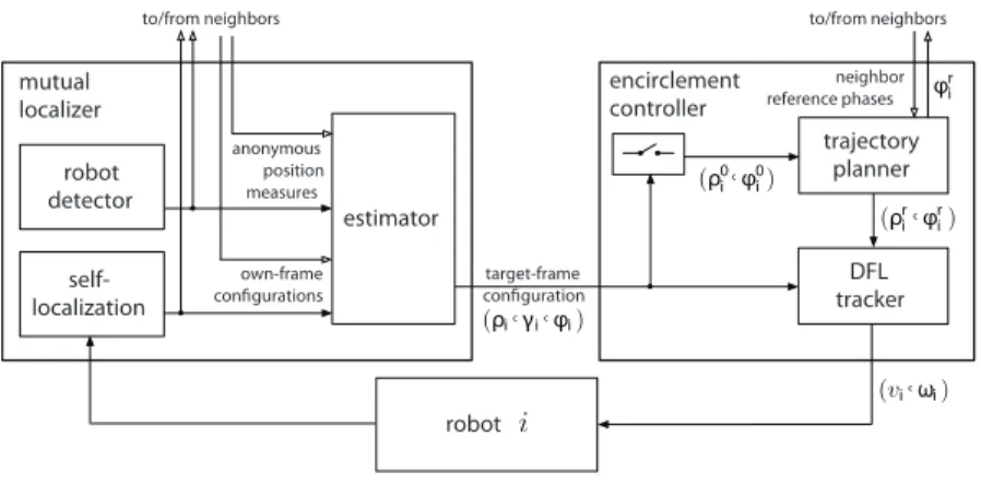
3 Formation control: the encirclement case 37 3.1 Introduction . . . 37 3.2 Problem setting . . . 40 3.3 Mutual Localization . . . 42 3.4 Orbital Controller . . . 43 3.4.0.1 Encirclement – Version 1. . . 45 3.4.0.2 Encirclement – Version 2. . . 45 3.4.0.3 Encirclement – Version 3. . . 46 3.5 Tangential Controller . . . 47

3.6 Conditions for Task Achievement . . . 52

3.7 Experiments . . . 53

3.7.1 Experimental results - Orbital controller . . . 55

3.7.2 Experimental results - Tangential controller . . . 55

4 Data fusion with the Transferable Belief Model approach 63 4.1 Introduction . . . 63

4.2 Transferable belief model . . . 65

4.3 A Transferable Belief model applied on formation pattern selection . . . 67

4.3.1 Problem setting . . . 67

4.3.2 Environmental categorization . . . 67

4.3.3 Simulations . . . 69

4.4 Distributed TBM for multi agent systems . . . 71

4.4.1 Problem Setting . . . 72

4.4.2 Static version . . . 74

4.4.3 Dynamic version . . . 84

4.4.3.1 Local Aggregation . . . 85

(13)

CONTENTS

4.5 An experimental case: the topological map building . . . 95

4.5.1 Problem Setting . . . 96

4.5.2 Environmental Patterns . . . 97

4.5.3 Local Topological Features Extraction . . . 100

4.5.4 Local Topological Map Building . . . 100

4.5.4.1 Topological Maps Aggregation . . . 102

4.5.4.2 Computational Complexity and Implementation Details 104 4.5.5 Experimental Results . . . 104

4.7 Example of Distributed Data Aggregation . . . 110

5 A stigmergic approach for environmental monitoring 115 5.1 Introduction . . . 115

5.2 Background . . . 117

5.2.1 Olfaction maps . . . 117

5.2.2 Building the artificial gradient . . . 120

5.3 Building the map . . . 120

5.3.1 Phase I : map seeding . . . 121

5.3.2 Phase II : gradient map . . . 123

5.3.3 Simultaneous building: the Olfaction gradient map . . . 124

5.4 Experimental results . . . 125

5.4.1 Experimental setup . . . 126

5.4.2 Data set validation . . . 128

5.4.3 Mapping with no obstacles . . . 128

5.4.4 Mapping with obstacles . . . 129

5.4.5 Concurrent seeding . . . 131

6 Static Sensor network localization: an initial step toward integration between static and mobile systems 135 6.1 Introduction . . . 135

6.2 Probabilistic localization . . . 137

6.3 Problem Setting . . . 139

(14)

6.4.1 Distributed Complete EKF . . . 141 6.4.2 Local EKF . . . 142 6.4.3 Compressed EKF . . . 142 6.5 Experiments . . . 143 6.5.1 Simulation tests . . . 143 6.5.2 Experimental tests . . . 144 6.6 Conclusion . . . 148 7 Conclusions 149 Bibliography 151

(15)

Chapter 1 Introduction

In the last years, Multi robot systems have gathered a lot of interest. This topic

represents the 9_{− 10% of the titles in the IEEE International Conference on Robotics}

and Automation in the last decade.

The great advantage in using multi robot architectures resides in an enhanced ro-bustness, flexibility and efficiency with respect to monolithic structures. The usage of multiple units intrinsically allows a greater resiliency to faults, a parallelization of the task execution among multiple agents and consequently a shortening in time execu-tion. The development of these systems has gone hand in hand with the technological improvements in the micro-machining fields. Nowadays the miniaturization, i.e. the en-ergy consumption reduction, allows the development of intelligent electro-mechanical devices keeping low the costs. Current embedded CPUs can run standard OS and consequently can mount conventional sensors/devices. De facto, these robots can be considered like small wireless units equipped with a considerable computation power.

The enhancement with respect to single robot architectures relies largely on the ability of exchanging information by wireless channels. In this manner, the team can instantaneously have a perception regarding different zones and consequently achieves a better understanding of what happens within the operating scenario.

On the other side, such advantages are paid with sophistication in the dynamics involving the overall system. This architecture can be represented by a set of simple, possibly different, systems linked each other by communication channels.

As a consequence, the stability of the algorithms running over a distributed system is much more difficult to analyze with respect to the past. Indeed, the communication

(16)

topology, which in most of cases changes rapidly over the time, couples the dynamics of the interconnected systems.

In last years, a big effort has been given to the study of ”networked” systems, especially those concerning coordinated motion and the data fusion.

The first topic aims at moving a set of agents in a coordinated manner while the sec-ond one tries to achieve useful considerations taking into account observations coming from different units, possibly dislocated over the operating scenario.

1.1 Movement control

The motion ability is one of the distinctive features of a multi-robot system with re-spect to conventional sensor networks. While the control for a single agent has been deeply studied and can be considered an achieved goal by the scientific community, the extension to multiple units is still susceptible of improvements.

The proposed techniques can be currently divided into two main areas: the first one tries to steer the agents into precise geometrical shapes by means of analytical control laws, while the second one finds inspiration from the biological world.

The former approach results effective to mathematically characterize the behavior of the system in terms of stability. However these algorithms rely on assumptions which hardly fit real scenarios, although they are very precise and well posed.

The bio-inspired algorithms instead aim to create an emergent behavior. They are based on the principle that local interactions, based on very simple rules, can lead to a complex global behavior when a large swarm is considered. With respect to analytical approaches, the convergence properties are rather difficult to demonstrate even if results can be very impressive.

However, in both cases the interaction between agents plays the fundamental role. The interaction is mainly based on the sensorial and communication capabilities of the robots.

Sensors are important in order to gather relative information, e.g. distance and possibly angular displacement, among agents. They vary from simple noisy transducers to sophisticated and expensive range finders which are able to gather very precise measurements. The kind of measures and their quality directly influence both the control design and the quality of the movement.

(17)

1.2 Sensor fusion

The kind of communication is instead strictly related to the task time comple-tion: power transmission and bandwidth tune the propagation speed of the informa-tion among agents. As for the sensors, these devices can be very simple, e.g. a light emitter, or very expensive, e.g. a large-bandwidth modem. Besides performance and costs analysis, a particular care about power consumption has also to be taken into account: especially when small devices are considered, the capacity of accumulators plays a fundamental role in the overall design.

1.2 Sensor fusion

Data fusion is a fundamental topic in robotics and in the overall scientific community. To have a full autonomy, a robot has to effectively process the data gathered by sensors in order to decide what to do.

Multi agent systems naturally enlarge the amount of information that a unit has to process: data coming from different places allow a better understanding of what is happening in the operating scenario.

This advantage is paid with sophistication in the model description: the estima-tion processes running on each robot are coupled by means of wireless communicaestima-tion channels.

Furthermore, this coupling, i.e. the topology of the communications, is dependent on the transmission capabilities and on the movements of the robots, i.e. it can rapidly change over the time.

In last years, a big effort has been made to study the behavior of these systems: a large amount of studies exploits the Bayesian framework. It allows a straightfor-ward combination of data coming from different sources. In this context, a multi robot system can be modeled like a network whose nodes are the robots and the edges rep-resent the communication links. Each node samples a given probability distribution and consequently fuses data coming from other sources by the probability theory. This approach is very effective when the probability distributions can be described by spe-cific characteristics, i.e. the noise affecting the transducers can be described with a Gaussian function. In this case the approach is computationally efficient and very easy to implement. However, even in this case, the topology of the communication links can lead to complicate situations which have to be carefully taken into account.

(18)

If the Bayesian framework provides an effective and easy-to-implement method to process data gathered from transducers, on the other side it does not provide the same expressivity in high level reasoning. For example, its rigid structure does not provide a natural representation of contradiction between sources. Furthermore, it difficulty handles the concept of ignorance: when an ambiguous measure is considered, typically the amount of belief is equally split among the most prominent hypotheses; this approach, for example, differs from the human kind of thinking which takes into account the union of prominent hypotheses and not its specifications.

Related to these situations, alternative frameworks have been proposed in liter-ature. These techniques describe an effective paradigm in cases where complex, i.e. contradictory and ambiguous, situations raise. However, this flexibility is paid with a huge increase of the computational burden. This is the main reason why they are often relegated to monolithic and static structures. On the other side, the advent of multi agent systems may naturally enhance the execution of these techniques. Currently, the application of alternative paradigms over distributed systems is still an open field susceptible of improvements.

1.3 Contributions

The main contributions of this thesis can be stated in three points.

The first one concerns about the prototyping of a mobile platform. This robot, replicated in 12 units, has been designed in order to execute multi robot algorithms. Differently from commercial platforms, this architecture is fully accessible in terms of control software and can be easily adapted to several scenarios without the insertion of adjunct boards. These peculiarities are demonstrated by several experiments which are described in this dissertation. At the moment, related publication about this topic has been published in (1). Currently, (2) has been submitted.

The second contribution is related to the formation control: in particular the encir-clement problem is treated. This topic has been deeply studied and many techniques have been proposed over the years. However, the majority of the algorithms require the knowledge of certain parameters which are difficult to estimate: to overcome this drawback, an external and centralized monitoring system is often used. In this disserta-tion, a fully autonomous multi robot system has been considered. Furthermore, control

(19)

1.3 Contributions

laws have been designed in order to avoid the use of parameters which are particularly sensitive to error estimate. At the moment, the related publication about this topic is (3).

The last contribution is related to data fusion. In this context, a big effort has been given by the scientific community to the enhancement of the Bayesian framework for multi robot systems. In this thesis, the Bayesian approach has been used in the domain of environmental monitoring in combination with a stigmergic approach in a smart environment. In particular, extensive experiments concerning the gas source localization have been conducted. Another contribution relies on the study of non-conventional paradigms in multi agent systems: in particular, an algorithm concerning the data fusion upon the Transferable Belief Model framework is presented. In this case as well the algorithm is supported by real experiments concerning the cooperative topological map building. At the moment, the related publications about this topic are (4), (5), (6), (7). Currently, (8) and (9) have been submitted.

In the final part of the dissertation, some notes are devoted to the integration between static and mobile systems. The related chapter does not pretend to go in deep about this topic: it just presents some preliminary technique about the static sensor network localization. In particular, this task can be viewed like a fundamental prerequisite in order to achieve the aforementioned integration. Before starting any task execution, in fact, a static sensor network has to know the location of the nodes. Here we propose a discussion about a distributed technique based on the Extended Kalman Filter. The algorithms are supported by experiments conducted using real

(20)

(21)

Chapter 2 An experimental platform for

multi robot algorithms

In this Chapter a mobile platform built from scratch is described. The main peculiarity relies in its flexibility: it mounts several sensors and others can be added in order to cope with several scenarios. A particular care regarding mechanical and electrical design has been taken in order to keep low the costs. Furthermore the communication capabilities allow the interaction with standard sensor networks. All these components are managed by dedicated software architecture

2.1 Introduction

A rather new and very interesting research field in mobile robotics investigates the cooperation of several units and in particular the possibility of getting a collaborative behavior by decentralized algorithms. Indeed, decentralized algorithms show definite advantages over centralized ones. They are naturally resilient to one point failure (the loss of one unit), can easily reconfigure themselves and don’t require a leader in the team. Moreover, they can take benefit from the increase of computing power that can be achieved parallelizing the activities of all the computers of the team. At the same time, the number and the length of inter-robot communications can be kept smaller than those necessary for centralized activities.

The field of decentralized algorithms can be roughly divided in two areas. The first and older one is that of swarm robotics where the control is performed by rule-based

(22)

de-signed behaviors (e.g. (11), (12), (13)). Tuned by a trial and error approach, they can provide a very good performance and can be adapted to different robots and environ-ments. Research works in the other area try to decompose well posed (in an analytical sense) algorithms in fragments that can be run onboard each robot using its small computing and communication capabilities (e.g. (14), (15)). Under these regards, the latter area shows several similarities with sensor networks and can even be useful to consider each robot as a moving node of such a network. The analytical demonstration of their convergence to the correct results is often carried on under milder assumptions than their centralized relatives and often assuming far from reality characteristics as Gaussian, zero mean errors, lossless communications, strict inter robot synchronization. In both cases, the results are strongly influenced by the available onboard sensors, the reliability and the range of the communication system and obviously the working en-vironment.

A serious assessment about the effectiveness of these algorithms requires therefore a good deal of experimental work and a team of robots. Thus, our research group decided to develop a prototype of a mobile robot that is low priced, in order to be replicated in many copies, and at the same time is equipped with many sensors, able to communicate over different channels, endowed with a sufficient computing power and easy to program.

SAETTA has been designed to fit these requirements. To have a low cost, we made some mechanical choices that positively influenced also the electronic part. The first is to build a standard differential-drive wheeled robot for indoor use and give up interesting, exotic locomotion approaches that are useful in more challenging environ-ments. Low cost derives also from the recent improvements of computer boards and even more from the advance of micromachined sensor technology. Several kinds of kinematic transducers are indeed included in the design, the utility of which will be discussed in the sequel. Moreover, we gave up any aesthetic concern, at least till now. The size of the robot was chosen in order to conduct experiments in a limited space with, say, ten units but at the same time sufficiently large to require no complex (and costly) miniaturization and to allow a few limited expansions.

(23)

2.2 Mechanical and traction design

Figure 2.1: Saetta robots: a part of the 12 Saetta robots developed at DIA.

Figure 2.2: The Saetta robot: along the body IR sensors are visible, while in the rear part, above the cap, the compass is located. On the top, a beacon allows to acquire the ground truth for performance comparison by an external camera.

2.2 Mechanical and traction design

The traction system of the robot and its mechanical structure play an important role in keeping simple the overall project and low the cost of each unit. One important choice has been the use of stepper motors instead of the more common d.c. ones. They offer several advantages. First of all, a stepper motor needs neither a tachometer nor an encoder nor, as a consequence, the circuitry associated with the transducer. As for the controller, the situation is not so clear, as a stepper motor requires no kinematic control loop, but it implies a rather complex timing, in particular when micro-stepping is used.

(24)

Thus, for this specific point, the difference is made by the hardware resources of the control processor that, in our case, are sufficient to perform all the needed operations. Moreover, a stepper motor requires lower supply voltages as it has a very low back EMF; this means less cells in the accumulator and a simpler circuitry. Finally, the provided torque is sufficient to move the robot without a gearbox even using large diameter wheels.

On the other hand, a stepper motor leads to longitudinal vibrations whose level has been kept low by a proper choice of the motor and of the driving technique (see Section

2.4.3).

The case of the robots has been kept as simple as possible without paying attention to the aesthetical results. We started from a standard PVC wiring box that is cheap and offers a sufficient mechanical robustness. Its rigidity, already good when the cover is inserted, has been enhanced by an internal aluminium bar that also carries the accumulators while the motors are screwed on the long sides of the box. The motors can carry a rather heavy transversal load that is several times the weight of the robot. Therefore, they can be placed so that the center of gravity of the finished unit is about aligned with the motor axes that support the wheels. In this way, a simple plastic sphere can be used for the third rest avoiding the use of a castor. The castor has been coupled with a small part of neoprene which acts like a damped spring. This choice was evaluated in order to reduce the amount of longitudinal vibrations induced by the stepper motors which resulted in a discontinuous floor/sphere contact. In this way the vibrations do not disturb the motion of the robot, that indeed shows a very good

odometry. The relevant data of the robot are referred in Table2.1.

Table 2.1: Robot specifications

Size 14_{× 29cm}

Battery voltage 9,6 V

Current consumption 600_{÷ 1000 mA}

Wheel radius 3.6cm

(25)

2.3 System architecture

The electronics of the robot is organized as a two tiers architecture. The first tier takes care of motors and sensors while the other one executes higher level control and communication tasks. This conceptual division has an immediate correspondence in the hardware realization: each tier is realized on a separate electronic board and has its own CPU.

The first board is custom designed around a Programmable Interface Controller (PIC) while the other is a commercial ARM9 board running embedded Linux (NETUS). The two boards communicate via a high speed serial interface. Interboard connectors provide, besides the electrical connections, the mechanical support to the ARM9 board. At the moment, a 2 axis gyroscope, a 3 axis magnetometer (only two used), a 3 axis accelerometer and 5 infrared (IR) sensors are connected to the lower level board.

2.4 Low level tier

This tier is implemented on a 18F87J50 PIC from Microchip. It is hosted by a board

whose size is approximately 13_{×27cm that, besides the CPU, accommodates the sensors}

(that are actually mounted on mini piggy-backs), the motor drivers, the power supply and the connectors carrying the other board.

The power source is constituted by the series of 8 AA cells providing a nominal voltage of 9.6V and a total capacity of 2.3Ah. Two supply voltages are needed: 5V and 3.3V. The conversion from the battery pack voltage is obtained by the cascade of two high efficiency converters. The overall autonomy depends on the characteristics of the experiment, i.e. the traversed space and the used peripheral and sensors. On average, the robot has a 90-minutes autonomy.

The board can work in a stand-alone way when the ARM9 board is not installed, connecting the PIC by jumpers to a dedicated connector for a wireless ZigBee module, thus obtaining a simpler but cheaper configuration.

2.4.1 Central processing unit tasks

The PIC is an 8 bit controller. The main features which are interesting for the project are detailed below:

(26)

Figure 2.3: System architecture: each peripheral is connected to a specific controller. The two controllers are linked (red arrow) by an RS232 communication.

• Clock frequency 48MHz • Supply voltage 3.3V

• Flash program memory 128KB • A serial RS232 communication port • 12 analog inputs with 10 bit converter • 4 timers/counters

• several digital I/O lines

A timer has been used to trigger the control cycle TP IC of the processor, in our case

25ms. The control period is responsible for managing the synchronous operations like channel sampling, data filtering and the coordination with the high level tier.

The main activities the PIC has to perform are: transducers sampling, control of the actuators by means of digital lines and communication with the high level tier and eventually with a ZigBee module if no upper level tier is used. In the latter case, the PIC is also used to run all the subtasks of the mission.

Asynchronous operations, like actuation and communication management, have to be taken into account, too. To this aim, some interrupts originated by the internal PIC hardware are used: the related description is detailed in Section 2.4.2.

(27)

2.4 Low level tier

2.4.2 Software

The software architecture is similar to the interrupt design pattern described in (16). The program is constituted by two main blocks: an infinite loop that executes low speed operations, and a very frequent and short routine. The latter is triggered by a timer which expires every 50µs: it checks for events related to some peripherals (serial port, motors, analog sampling, etc) and, if needed, it performs some fast actions (setting a flag, buffering of a received character, step movement, storage of acquired data, etc). It performs only very simple operations and is not preemptive.

Flags enable the execution of slower operations in the infinite loop: if a flag is set, the launch of the related long term action (like message parsing, notification of served positions, data filtering, etc) is performed.

2.4.3 Motor Control

Each motor is controlled by a dual full-bridge pulse width modulation (PWM) driver. The driver is a 24 pins dual inline package (DIP). It provides both electrical and thermal protections. Stepper motors provide a 200 steps resolution with a nominal torque of 12 Ncm. The motor windings are independently controlled: four current levels can be imposed, ranging from 0% to 100% of the max current value. The control is done acting on a couple of pins controlled by the PIC. Furthermore, another pin is used to impose the current direction in the winding. Globally, six digital lines per motor are used by the PIC to perform the control which results in a PWM of fixed period. The electrical period is at least constituted by four intervals. When using micro-stepping, the intervals are multiple of four and in our case eight or twelve intervals have been tested. As a

consequence a resolution respectively of 400 and 600 steps can be achieved. Figure2.4

shows the vibration analyses on the mechanical structure for these two kinds of control when the wheel rotates at 2.5Hz. Data were collected by a Type 4371 accelerometer from Bruel & Kjaer. The twelve intervals solution clearly shows lower vibration levels and it is used for the whole range of operation even if it is slightly more demanding in terms of CPU operations. As a result, the robot odometry on a typical floor is very good. After estimating the wheel diameter by calibration, the error along a straight line is less than 1%.

(28)

0 20 40 60 0 2 4 6 8 12 steps 8 steps Hz

Figure 2.4: Vibrations gathered with twelve (continuous blue) and eight intervals control (dotted red). On the x-axis Hertz units are represented while on the y-axis the magnitude of the signal gathered from the accelerometer is showed. The eight intervals control shows a peak centered at about 20Hz.

2.5 Sensor characteristics and calibration

The robot is provided with a rather complete set of kinematic sensors. In particular, the proprioceptive ones are a 3-axes accelerometer, a 2-axes gyroscope and a 3-axes magnetometer (to be used as a compass); odometry sensors have not been included as stepping motors are used. The range of exteroceptive sensors connected to the PIC comprehends just five IR range finders as more sophisticated units are driven by the upper tier processor. In this tier, the transducer furnishes analog sources which are sampled by the analogical to digital converter provided by the PIC. When needed, a small circuitry constituted by an amplifier and low pass filter is put between the transducer and the PIC.

All the channels are sampled with a burst acquisition: in each control cycle TP IC,

the PIC collects N (in our case N = 8) samples for every channel at maximum sampling

rate (60− 100µs per channel). The acquisitions are then averaged to reduce random

fluctuations. It is worth noting that the number of samples is a power of 2 to improve the computation time using shift operators.

In the following the aforementioned sensors are described, together with their per-formances and calibration, when needed.

2.5.1 Infrared sensors

Each infrared sensor, a GP2Y0A02YK from Sharp, is composed by an emitter and a separate detector. The analog range measurement is obtained by a triangulation of

(29)

2.5 Sensor characteristics and calibration

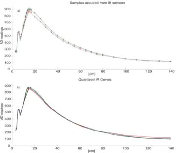
the spot projected on the obstacle. Intensity is discarded, thus the sensor is insensitive to the obstacle reflectance. However, differently from the other sensors mounted on the robot, the relation between the output voltage of the sensor and the distance is not monotonic and shows a maximum near 20cm. Therefore the same reading can

refer to two different distances (see Figure 2.5-a) and this ambiguity is located in a

range that can be very dangerous with respect to the safety of the robot (e.g. collision avoidance). Thus, a dangerous and safe zone must be considered in the IR curve. One way to overcome this problem is considering subsequent readings to disambiguate from the two zones. For each unit, the calibration was effected using a standard polynomial

fitting considering a separate subset of data for each zone. As shown in Figure 2.5

-a, a small difference results between the tested units, however it can be reduced to acceptable values by a simple vertical translation of the calibration curve: the result of

this operation can be viewed in Figure2.5-b. The operative range can be considered to

be from 7cm to 120cm: out of this range, measures are useless due to the noise and the discretization of the converters. Errors are particularly important for distances greater than 80 cm: the standard deviation of the measure, even averaging 64 samples, is near 10cm and affects in particular localization and mapping tasks. Instead, for distances between 25cm and 50cm, the repeatability is about 1cm. Along this range, the mean error is under 2cm.

Each IR sinks about 50mA, thus the PIC can turn ON or OFF their supply line by a transistor.

2.5.2 Accelerometers

The accelerometer device is a 3 axes unit (MMA7260QT from Freescale semiconductor). Its range can be chosen among four values from 1.5g up to 6g by 2 pins. This setting is typically applied at power up, but online changes are possible. Actually, considering the noise superimposed to the measures and the difficulty to get rid of the offsets, these sensors cannot be reliably used for velocity or position estimation and they find the main application to state the position with respect to the horizontal plane, an information that can be very useful in connection with the sensors connected to the upper tier, e.g. the camera. In particular, supposing that initially the robot starts the mission on a horizontal plane, a different posture is recognized if the values gathered on the axes differ from the initial ones. To this purpose, the maximum sensitivity is

(30)

Figure 2.5: Calibration curves obtained from different sensors: (up) original data; (down) curves after the unbiasing. Y axis are AD units, on the x axis distance in cm is reported.

used. As in this case two axes are sufficient, it is possible to leave out one axis by a jumper (the one oriented along the non-holonomic constraint of the vehicle) to sense the battery voltage.

2.5.3 Rotation sensors

This section briefly describes the behavior both of gyro and magnetometer sensors. The gyro is a 2-axes ADXRS150 sensor from Analog Devices, oriented along the roll and yaw axes of the robot. At the moment, the most used part is the one oriented along the yaw axis, which measures the rotational speed of the robot.

The magnetometer is a three-axes HMC1043 sensor from Honeywell. To spare an analog input, only two axes were considered, being them sufficient to determine the position of the Earth magnetic field on the horizontal plane. To adapt the chip output levels to those of the analog/digital converter, two operational amplifiers are needed. The two components can be affected by a bias related to the residual magnetization of the sensitive core. Each of these biases cannot be estimated as they change randomly at every power-on. To overcome this drawback, a calibration, consisting in a full self-rotation of the robot, has to be performed at the beginning of each experiment. Alternatively, the magnetometer provides a procedure consisting in a reset driven by

(31)

2.5 Sensor characteristics and calibration

a train of current pulses injected into a digital line of the chip. Although effective, in our case the amount of current needed by this operation is too much onerous for the battery capabilities.

Also in the case of gyro, a calibration at each power-on is performed by self-rotations. The gyro calibration curve revealed a linear behavior with respect to the rotational velocity of the robot (see Figure 2.6).

The magnetometer outputs instead showed the expected profile: each axis returned a sinusoidal curve representing the projection of the magnetic field on that direction. Two remarks are in order: first, the currents flowing in the robot’s circuits has a negligible effect on the readings of the magnetometer; second, the gyro is very sensitive to temperature conditions. In our experiments, we noted that these variations were not negligible. In order to reduce this phenomenon, we tried to estimate the bias whenever the robot stopped: tough that some improvements was obtained, the gyro did not result reliable over long periods to achieve velocity and nevertheless position measures, especially over long periods.

Consequently the velocity integration is unreliable on long time intervals.

During the navigation experiments, however, the two sensors showed rather different error characteristics. While the gyro maintained the expected behavior, the compass resulted unreliable in some areas of the arena where experiments were performed: these situations were observed when passing over big iron beams installed under the floor.

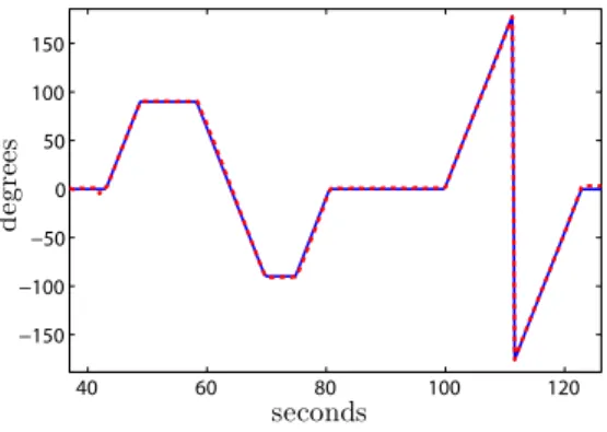
One typical behavior is depicted in Figure 2.8. In this test, SAETTA traveled two

straight paths interleaved by a 90 degrees rotation. During the self rotation, the field direction was constant and the angle was correctly measured (the sensor returned 88.8 degrees); on the contrary, during the straight paths, the reading exhibited large errors because they passed over a beam that modified the magnetic field. Obviously, any large ferromagnetic mass induces the same problems. When no disturbing mass is present, the compass is highly reliable as can be seen by Figure2.14. In this graph the magnetometer measures are compared with the odometry ones that can be considered reliable due to the very slow velocity imposed to actuators. The maximum error in this experiment was 7o.

Thus, we can have some indications on the use of the two kinds of sensor. When self rotating, compass is reliable for rotational measures but cannot provide an indication of the absolute position of the robot wrt the North direction. Absolute angle can be

(32)

400 420 440 460 480 500 −1.5 −1 −0.5 0 0.5 1 1.5 ra d/s digit units

Figure 2.6: Calibration curve for the gyroscope sensor: red asterisks represent the mea-sured data, the blue line is the calibration curve achieved by the least square estimation. Robot rotation speed is on the y axis (radiant/sec), digit units on the x one.

40 60 80 100 120 −150 −100 −50 0 50 100 150 d eg re es seconds

Figure 2.7: Magnetometer measures compared with the bearing achieved by odometry: continuous line (blue) is the odometry of the robot, dotted line(red) is the magnetometer reading. The signals are expressed in degrees units over a temporal scale (seconds). The maximum displacement is about 7 degrees.

relied upon only if there is an a priori knowledge about the presence and the position of disturbing masses, or after a long straight path during which the compass readings are constant. Moreover, the compass can be used to go back on a path already followed, as in each point the error is the same in the two ways. For paths with a sufficiently fast velocity and a large radius of curvature, it is safer to rely on the integration of the gyro readings if the bias can be estimated in some way (for example during stop phases).

(33)

2.6 High-level tier 0 20 40 60 80 100 120 −0.5 0 0.5 1 1.5 ra d seconds

Figure 2.8: Curve acquired by the magnetometer: continuous line (blue) is relative to straight motion affected by iron beams, the dotted (red) one is relative to a self rotation of π/2. Signals are represented in degrees units over a temporal scale (seconds).

2.6 High-level tier

The high level tier is implemented on a Linux embedded board, the NETUS board from ACME SYSTEMS srl. It has an AT91SAM9G20 Atmel processor at 400MHz. The board comes with 64MB RAM and 8MB FLASH. It sinks 60mA from a 5V source and offers 5 serial, 2 USB and 1 ethernet ports plus several digital input/output lines. It carries an expansion board hosting a ZigBee module for communications in an un-structured environment. Linux offers the advantages of a solid open source Operating System that can be tailored on the user needs and gives the possibility to easily access the low level resources. The availability of many widespread interfaces as the USB and the RS232 in a standard OS opens the system to the use of an almost unlimited number of peripherals. At now we have connected webcams for vision and inter-robot distance estimation, standard Wi-Fi keys, an RFID tag reader for navigation in par-tially structured environments and a small laser scanner. With a careful programming, even rather complex vision algorithms can be implemented and, at the moment, the actual bottleneck seems to be in the batteries, since all these expansions sink a lot of current.

2.6.1 ZigBee communications

In a multirobot scenario, the ZigBee wireless communication channel is very important for the system architecture. In particular, the ZigBee module from Maxstream has

(34)

been used. This module can communicate with a baud rate up to 250000bps within a range up to 20m in an indoor environment and up to 100m in outdoors without

an infrastructure 1. The protocol enables the robots to interact also with ZigBee

compliant sensor networks. The use of this chip makes it possible to embed SAETTA in etherogeneous systems including both sophisticated devices as well as tiny platforms (see for example (17) ) .

Differently from Wi-Fi devices, ZigBee ones have low power consumption: supplied at 3.3V, our module sinks 55mA and 270mA respectively in RX and T X modes and less than 1mA when idle. On the contrary, they show a smaller bandwidth that is anyway more than sufficient for most cooperation purposes.

Furthermore, several options using the ZigBee API are available. It is worth to underline the main features related to the typical multirobot scenarios. The module is able to work in different modes, which can be switched at run time: sleep, receive, transmit, idle and command mode. The last one allows the master device to set con-figuration parameters of the chip. Furthermore, it is possible to establish either a connection with implicit management of the acknowledgement (similar to TCP/IP) or without it (similar to UDP) depending on the specific application. Due to the cost of transmitting a packet, it is possible to send data in a broadcast mode or to a specific subset of other nodes (specifying the Personal Area Network ID to which the nodes of interest belong). These options (that are completely managed by the module without further computational load for the processor) find a direct correspondence in multi

robot applications where the communication graph plays more ((18)) or less ((19))

importance, requiring a strictly connected net or a sporadic exchange of information without acknowledgements.

When an interaction both with sophisticated hardware and with a sensor network is required in the same experiment, it is possible to use at the same time both the ZigBee (802.15.4 standard) and the standard Wi-Fi channels (802.11 standard).

2.6.2 Software

Relying on a Linux OS, the software architecture has been developed in a more sophis-ticated manner than the PIC code.

(35)

2.6 High-level tier

In literature several frameworks have been proposed. In (20), the Player project is introduced. It is a multi robot framework where each robot can be seen like a node of the network. Even in the internal architecture of each agent, devices and algorithms can be implemented as nodes connected each other: this approach is very effective in terms

of abstraction but has the inconvenient in the overhead of communications. In (21)

an interesting approach to domestic robotic networks is described: in this framework, every piece of data, referred as ”a tuple”, is ”published” in a distributed and connected network. Also in this case the overhead introduced into the communication was not appropriate for tiny devices. To overcome this issue, an optimized version running even

on very limited platforms is described in (22). Another interesting approach is given

in the Multi-Robot Integrated Platform(MIP) 1_{: this framework is an object oriented}

environment which divides algorithms, tasks and devices into categories. Within each category, a component can be easily substituted by another one, resulting in short time-to-develop new experiments. Furthermore the algorithms can be executed both on real platforms (Khepera III) and in a simulated environment based on Player: the swapping between the two environments is easy as the change of one flag. Although very flexible, the use of OOP programming introduces an overhead which highs the computational burden, especially for embedded platforms like the one used on SAETTA.

In our case, we have chosen to develop a framework which encompasses both the overhead about sophisticated communications and OOP programming. A particular care about the timing performances was taken at the price of losing the abstraction level previously described.

The developing system is based on the C language. Our board mounts a standard Ubuntu 9.10 version, thus we could take all the advantages of the standard programming techniques. Currently, we chose a multi-threading approach to separate the kind of activities to be executed.

The critical ones are put in the main thread. This thread has a cyclic structure whose period is 200ms. It contains the routines to communicate with the PIC, motion commands and all the subtasks which concern about the safety of the robot. The control period is triggered by an interrupt deriving from the interface with the PIC

(see Section2.7) which starts the communication exchange between the two CPUs.

(36)

200ms MOTOR CONTROL LOW LEVEL DATA PROCESSING ZIGBEE MAIN THREAD COMM THREAD GENERIC THREAD SV SV PIC COMM MOTOR CONTROL LOW LEVEL DATA PROCESSING PIC COMM ZIGBEE ZIGBEE … … … … … … ZIGBEE INT INT t

Figure 2.9: High level program structure: on the left the vertical time line is depicted. The first block, the main thread, is constituted by the periodic execution of subtasks: the communication with the PIC (PIC COMM block), motor control, and low level data processing. It can be seen that the periodicity of this thread is triggered by the interrupt INT which raises every 200ms. Conceptually, other parallel periodic threads can be run at the same time: they can be executed by subtasks whose execution can be shorter than the control cycle (e.g. COMM THREAD) or longer (GENERIC THREAD). The communication between threads is performed by shared variables SV.

This thread can be flanked by other ones which contain auxiliary activities: cur-rently one is used for wireless communication (ZigBee or Wi-Fi), another for an RFID reader and so on. Typically each thread has a cycle which depends upon the activity it has to do: if a precise synchronization is needed, semaphores can be adopted. Com-munication between threads is implemented by the use of shared variables (see Fig.

2.9).

It is worth to note that whenever a thread doesn’t have to perform any operation, it is put in idle mode, i.e. it is not time consuming, by the OS (23).

2.7 Communication between the two tiers

The interaction between the two tiers, i.e. between the NETUS and the PIC boards, is

performed under the RS232 communication protocol. Denote with TN ET U S and TP IC

respectively the NETUS and the PIC control period cycle. The exchange of information

is made at the beginning of TN ET U S (see Figure 2.10). The starting message, sent by

(37)

2.8 Basic Testing TNETUS TPIC 25 ms 200 ms START COMMAND SENSOR DATA NETUS PIC HEADER PAYLOAD CRC a) b) 1 byte L byte 2 byte

END 1 byte

Figure 2.10: System timing. a) Communication process between the two controllers. The PIC sends a starting message (red arrow), the NETUS replies with a command (blue) and finally the PIC send processed data (green). b) Packet structures: header (1 byte ID), payload (varying length), a crc code (2 bytes) and an end character (END). The end character is unique as it cannot compare in the other fields: a masking technique is used to avoid this condition.

run. The NETUS board answers with a packet containing commands computed by the previous cycle. Finally, after receiving the command packet, the PIC board sends the data collected and processed over the 8 previous sub-periods. Each message, in both directions, is composed by the following fields:

• header: it is an ID that identifies the kind of packet • payload: it is the information owned by the packet • crc: it is a verification code

• end: it identifies the end of the packet

The commands that the upper tier can send are: system state conditions, refer-ence velocities or displacements and stop commands. The lower tier sends data about odometry, sensor readings and acknowledgments about correct command execution.

2.8 Basic Testing

In this section two simple experiments are described in order to show the performances of the platform. In each test the robot was asked to execute some well known task

(38)

in robotics. The first experiment is devoted to characterize the interaction between multiple units: robots have to meet in a common point using the consensus algorithm

(18). In this scenario both communication and odometry performances were tested.

The second experiment is related to infrared sensors: one robot explores a small area

in order to build a map of the surrounding environment. In Section2.9a more detailed

experiment about localization will be provided.

2.8.1 Consensus algorithm

In this scenario a set of 3 robots was used. The test was made to evaluate the perfor-mances of the system about motion precision in presence of heavy inter-robot commu-nications.

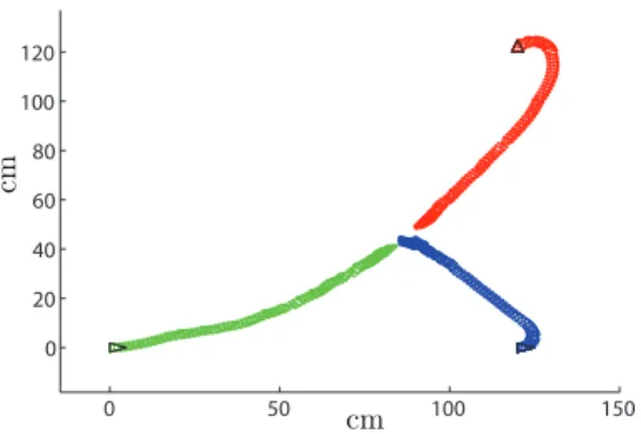
Each agent, having a prior knowledge of its own state with respect to a common frame, broadcasted repeatedly its position to the others. Applying the consensus filter, the robots would meet to the mean of the initial positions if the dynamics of the robots were linear. Due to the nonholonomic constraints, the input generated by this control

law had to be filtered by a Cartesian controller (24). As depicted in Fig. 2.11, this

controller overcomes the drawback: the trajectories of the robots converge to a common point, which obviously is not the mean of the initial states. In detail, in this test, each robot traveled meanly for 84.3cm: the maximum linear speed was set to 8 cm/s while the rotational one was 0.98 rad/s. Each robot broadcasted its state with a frequency of 10 Hz (double with respect to the control cycle to prevent data loss): on average

each robot sent 137 packets. In tab. 2.2it can be seen that the number of lost packets

is negligible as well as the computational load: the algorithm took about 3ms per iteration and could be furthermore reduced avoiding the use of trigonometric functions with lookup tables and integer implementations.

Similarly, the odometry furnishes precise data. Robots arrived to a common point without having feedback about their positions. As mentioned before, several tests revealed errors smaller than one percent over long straight paths (about 12m) and contained angular displacements as well.

2.8.2 Mapping

In this test a robot explored a small area to build a map by the IR sensors. In

(39)

2.8 Basic Testing

Table 2.2: Consensus experiment data

Robot 1 Robot 2 Robot 3

Path (cm) 59 98 96

max speed (cm/s) 7.54 7.36 7.25

mean speed (cm/s) 3.15 3.85 3.99

Packets sent∗ 129 152 130

Total data loss 3.5% 2.9% 2.1 %

Max data loss with respect to one target 3.7% 3.1% 2.4 %

∗_{different numbers of packets sent are due to different power-on time of the robots: the broadcasting is related}

to the power-on time while the consensus algorithm starts in a synchronous manner with an external starting command.

0 50 100 150 0 20 40 60 80 100 120 cm cm

Figure 2.11: Consensus algorithm for 3 agents: black triangles represent the robot initial positions. The axes units are centimeters.

dimensions were chosen in order to effectively exploit the IR sensors.

In the test the robot made a smooth trajectory: along a straight path it stopped for two times to span the surrounding environment. The results of this experiment can be

seen in Figure2.13. The maximum linear speed was likely 6cm/s with a mean speed,

without taking into account the resting, of 2.79cm/s while the maximum rotational speed was 0.3 rad/s.

The mapping results are good (see Fig.2.13): the sides of the open square are

estimated with an error less than 5cm without using any sophisticated data processing. When more demanding mapping is needed, more performing sensors, e.g. laser range finders, can be mounted on SAETTA.

(40)

Figure 2.12: Test bed for the map building: the sides of the square are 60cm long; the two slanted sides are 1m long.

−20 0 20 40 60 80 100 120 −50 0 50 cm cm

Figure 2.13: Map built by IR sensors. the robot trajectory is represented in violet, asterisks show the sensor acquisitions. Each color identifies an IR sensor: the front side ones are blue and red dots, front central one is yellow and the rear lateral ones are green and black.

2.9 A modified particle filter for low performance robotic

platforms

In this section a localization algorithm, for small platforms like SAETTA, is presented. These experiments were conducted with a previous version of the NETUS board, the FOX one mounting a chip of 100MHz, making the scenario more demanding. Due to the limited processing capabilities, some ad hoc solutions have been used: the lack of processing resources has been compensated by an efficient implementation of the estimator and by the use of compass measures which ease the computational load. The

(41)

2.9 A modified particle filter for low performance robotic platforms

results show how a careful design allows the implementation of sophisticated algorithms even on small platforms.

2.9.1 Problem setting

The localization problem can be approached using a probabilistic framework. It ba-sically consists in the state estimation of a system whose temporal evolution can be modeled as:

qk = f (qk−1, uk−1, νk) (2.1)

where k _{∈ N, f(·, ·) is a generic nonlinear function, q}k ∈ Ω represents the state of the

system at the k _{− th time step, u}k represents the control input, νk ∈ N(0, σν2) is a

zero mean Gaussian noise with variance σ2

ν and Ω is the set of all the states x. To

improve the estimation process, an observation system is used to gather measures that are function of the state x. It can be modeled as:

zk = h(qk, λk) (2.2)

where h(_{·, ·) is a nonlinear function and λ}k ∈ N(0, σλ) is a zero mean Gaussian noise

with variance σλ. It is assumed that the sequence of states qkcan be modeled as a first

order Markov process, e.g.

p(qk|Qk−1, Uk−1) = p(qk|qk−1, uk−1) (2.3)

and also that the observations zk are conditionally independent, hence:

p(zk|Qk) = p(zk|qk) (2.4)

where Qk represents the sequence of states up to the instant k. Similarly, denote with

Zk and Uk respectively the set of measurements and control inputs up to the generic

instant k.

Under the previous assumptions, a prior and posterior belief about the state estimation can be introduced. The first represents the degree of belief about a certain state based on the knowledge of the previous estimates, the control input, that is assumed to be

perfectly known, and the observations, all of them up to instant k_{− 1:}

(42)

the latter instead represents the degree of belief after acquiring a new measure zk; due

to the assumptions described by eq. 2.3 and eq. 2.4 and using the Bayes rule, the

posterior belief can be defined as:

bel+(qk) = p(zk|qk)bel

−_(q k)

p(zk|Uk−1,Zk−1) (2.6)

where p(zk|qk) is the perceptual model. In this way, the recursive estimation can be

performed by defining the prior belief as: bel−(qk) =

R

Ωp(qk|qk−1, uk−1)× bel+(qk−1)dqk−1 (2.7)

Particle filter adopts the aforementioned recursive model by a sampling approach. The posterior belief function is approximated by a set of N samples extracted by a normalized importance sampling distribution π(qk|uk−1, zk):

bel+(qk)≈ _N1 PN_i=1wi· δ(x − qi) (2.8)

where δ(·) represent the Dirac pulse, and qi, i ∈ 1, . . . , N is a sample extracted by

the distribution π which, in the robotics field, is commonly represented by the prior distribution bel−(qk) ((25)). Under this assumption, using the Bayes rule, the weight

assigned to each particle is:

w(i)_k = w(i)_k−1·p(zk|q(i)k )bel−(qk)

π(qk|uk−1,zk) = w

(i)

k−1p(zk|q_k(i)) (2.9)

Furthermore the prior belief can be achieved in a recursive fashion as:

bel−(qk) = p(qk|qk−1, uk−1)· bel+(qk−1) (2.10)

This recursive procedure has to be supported by a re-sampling technique. As new data become available, most of the particles have a negligible weight. These ones, with a re-sampling procedure, can be substituted with particles which fit better the new measures. To determine when a re-sampling iteration has to be done, the following performance index is commonly used:

Tk = PN 1

i=1(w∗ik)2 (2.11)

where w∗i_k is the normalized weight:

w_k∗i= _Pwik N i=1wik

(43)

Whenever this value is less than a constant T , a re-sampling process is started. This consists in choosing a new set of particles according to the distribution p(qk|Zk):

p(qk|Zk)≈PNi=1wikδ(qk− qki) (2.13)

in other words, the new particles are sampled with a major probability in the neigh-borhood of the most promising particles of the previous iteration.

2.9.2 Algorithm implementation

In this section the implementation of the algorithm on the SAETTA robot is discussed. In its complete formulation, for each particle the algorithm computes the intersections between the five beams originating by the infrared sensors and all the walls and then selects the feasible (shortest distance) intersection to compute p(zk|qk). These

com-putations involve multiple rototranslations, each of which makes use of trigonometric function. This kind of operation represent the main bottleneck in the algorithm exe-cution, thus the attention will be focused just on this part.

Denote with F0 the frame origin and omit the temporal index k. Let the generic pose

of the particle with respect to F0 be qi ={pi, θi}, with pi = (pxi p y

i)T ∈ R2 and θi ∈ S.

Furthermore denote with Fb a frame related to a generic sensor b = (pb θb)T ∈ R2× S,

centered at pb and oriented like θb with respect to F0. Similarly, let bz = (bpz bθz)T

the representation of the pose z∈ (R2_{× S) with respect to F}

b. It is assumed that each

particle i is equipped with M sensors (in our case M = 5), each of which having a pose sji = (qjiβji)T,j = 1, . . . , M , with respect to F0.

Consider a generic particle qi and define a fitness function g : R × R → R, for sji, as

the Gaussian: g(dj, ˆdji) = √1 2πσ2 s e (dj − ˆdji)2 2σ2s (2.14)

where dj is the measure actually acquired by the j-th sensor, ˆdji is the measure the

sensor would acquire if the robot were in the particle pose qi, and σsis a fitness function

parameter.

The most of computation relies on the determination of ˆdji. Consider a linear obstacle

Odelimited by the endpoints ξ1 = (ξ1x ξ1y)T and ξ2 = (ξ2x ξ2y)T, with ξ1, ξ2 ∈ R2. A

(44)

means of a rototranslation, the endpoints with respect to Fsji:

sji_ξ

o= R(−(βji+ θji))(ξo− qji), o = 1, 2 (2.15)

where R(_−(βji+ θji)) is the rotation matrix along the axis orthogonal to theR2 plane.

The computation of the distance is performed whenever at least one of the x coordinate is positive and the y coordinate of the two points are opposite each other. If these two conditions are satisfied, the distance between the sensor ji and the obstacle O is:

ˆ

dji|O =−sjiξ1y

sji_ξ_1x₋sji_ξ_2x

sji_ξ_1y₋sji_ξ_2y +sjiξ1x (2.16)

Consider the environment E = SP

i=1Oi like the union of the all P linear obstacles

present into the environment, P _{∈ N. To determine the expected reading of a generic}

sensor, its minimum distance from the obstacles in E must be considered; ˆ

dji = minp dˆji|O=Op (2.17)

where the term ˆdji|O=Op denote the distance between sensor pose sji and the obstacle

Op. The complexity for the determination of the distances for the whole population of

samples is O(N_{· M · P ). This requires a lot of computations and constitutes the worst}

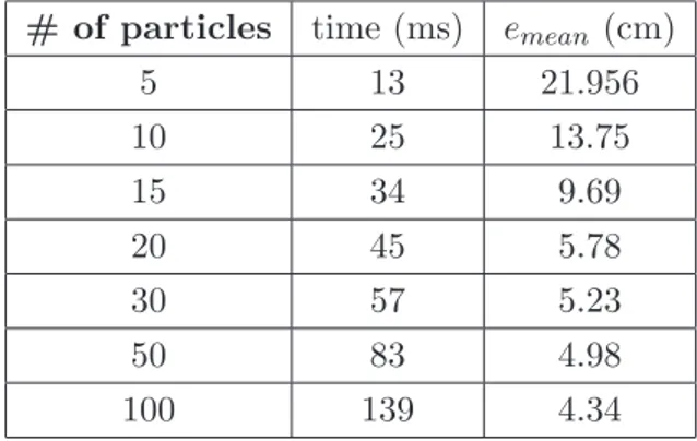
bottleneck of the implementation. Each iteration of the aforementioned algorithm, using floating point numbers, takes about 2.6s considering a population of 20 particles. In the optimized implementation, shown in the next section, the same iteration takes about 40ms.

2.9.2.1 Optimized algorithm

The efficiency improvements are based on three actions. The first one consists in using the compass readings to impose the particle bearings. The feasibility of this action is related to the precision shown by the compass, at least in our experiments. In this case the computing time for p(zk|qk) is only 1.5 seconds, which is about one half of

the original one. Note that the particle number (equal to 20) has been kept the same. Therefore it is used to span a 2-dimension space instead of a 3-dimensional one thus improving the particle “density” which in turn provides a smaller error and a better convergence of the algorithm as shown by the reduced number of effected re-samplings. Actually, to get the same properties of the original algorithm, this number could be reduced with a consequent improvement of the iteration speed.

(45)

Furthermore, because the execution time is still unsuitable for real time use, an

integer representation has been adopted (26) for the numeric variables and a lookup

table Tcos has been used for the cosine operator. These actions make much faster the

rototranslation of walls. In fact, every wall is rotated by the same angle given by the sum of the compass reading and the sensor relative angular position. It is worth of

note that the same approach is applied to shorten the computation of sji by rotating

the vector position of the sensor wrt the robot center of the angle.

In particular, being our scenario confined in few meters, the 32 bit length which is native of our processor for integer variables makes it negligible the loss of precision due to the quantization (27). As for the angles, the range from 0 to π/2 has been discretized into 128 levels. The correspondent cosine range, [1, . . . , 0], has been represented by the interval [1023, 0]. In this way a generic angle α is represented by an index l s.t. Tcos[l]/1023≈ cos(α).

This representation (26) is sufficient to represent the cosine of every angle into

the range [_{−π, π]. Similarly, the sine representation reduces by a proper shifting in}

the table. The same approach, obtaining the table Tf itness, has been used for the

computation of the fitness function in Eq. 2.14. Also the range of values which the

fitness function can assume has a maximum which is a power of two, thus reducing the normalization operator to a simple shift. It has to be stressed that this approach, making use of analytical representation for the environment, can be easily adapted to gridmaps. The schematization of the algorithm can be viewed in Alg. 1.

2.9.3 Experimental results

In this section some experiments are presented to show the performance achieved by SAETTA. The test bed is constituted by a rectangular arena which presents a recess

(see fig. 2.15). Several tests have been conducted: here we describe one of the most

significant. The ground truth about the Cartesian position of the robot has been logged by an external webcam calibrated by the Matlab Vision Toolbox. In this experiment the robot has traveled for about five minutes in the arena. Due to the stochastic nature of the particle filter, beyond the onboard real time implementation described before, the data collected by the robot were stored in a PC to perform also a statistical analysis of the behavior wrt different initial conditions randomly chosen to start the population of the particle filter. The comparison was performed between a standard particle filter

(46)

Algorithm 1: Fitness value for the particles population Data: dj, qi, sji , j = 1, . . . M, i = 1, . . . , N

let ˆθ be the compass measure

Result: f itness values ωi, i=1, . . . , N

for each sensor j=1, . . . , M do

get cos(_{−(ˆθ + β}ji)) and sin(−(ˆθ + βji)) from Tcos[l]

for each particle i = 1, . . . , N do ˆ

dji← ∞

for each Ok∈ E, k = 1, . . . , P do sji_ξ

o= R(−(ˆθ + βji))(ξok− pji), o = 1, 2, making use of Tcos[l]

if ( (sji_ξ

1x > 0 or sjiξ2x > 0) and (sign(sjiξ1y)6= sign(sjiξ2y)) then

compute daux according to eq. 2.16

if daux < ˆdji then ˆ dji← daux end end end

ωji = g(dj, ˆdji) making use of Tf itness(⌊dj− ˆdji⌋)

end end

for each particle i = 1, . . . , N do wi = _M1 PM_j=1wji

end

(PF) and the fixed bearing algorithm (FBA). Due to the reliability of the compass in our test-bed and the reduced dimensionality of the problem, the convergence of the FBA is

faster and the errors are smaller than the ones achieved by the PF. Table2.3has been

obtained running the algorithm on the same data set for 500 iterations (approximately 100 seconds) and starting from 50 different initial conditions. The error is relative to the weighted mean of the best five particles, in terms of importance weight, over a total population of 20. The FBA shows better performance than PF, both with respect to the error statistics and to the number of re-samplings. Running the standard algorithm with a bigger population, e.g. 50 particles, the results are, as expected, slightly better

(47)

2.9 A modified particle filter for low performance robotic platforms 0 20 40 60 80 100 120 −200 −150 −100 −50 0 50 100 150 200 s d eg rees

Figure 2.14: Magnetometer data compared with bearing obtained by odometry : solid line is the odometry of the robot, dashed line represents magnetometer readings. The units for y axis are degrees. The maximum displacement is about 10 degrees.). On x axis the time, in seconds, is reported.

but with a computation time almost twice as high. Some data concerning about time execution of the FBA algorithm with respect to the particle population are reported in Table2.6).

In Table 2.4, the results of the whole navigation are showed: also in this case the

FBA performs better with respect to the PF. The error trajectory for one trial is

de-scribed in Fig. 2.16: the curves represent the error obtained considering respectively

the weighted mean of the 5 best particles at each iteration and the mean of the total population. The correspondent representation of the first curve is represented in fig.

2.15. The red dots represent the mentioned weighted average; the isolated ones

repre-sent initial estimates and correspond to the first part of the curve. After 400 iterations, when the error starts to decrease, the best hypotheses track the robot trajectory. This situation is represented by the dense set of hypotheses lying on the neighborhood of the robot trajectory. Finally, a kidnapping test is showed. In this case, the data set

has been dropped from iterations 200 to 900. As detailed in Table 2.5, results show

how the FBA algorithm performs after about 500 iterations. In this section, we did not consider the Extended Kalman Filter because, although effective, this estimator needs to know the initial location of the robot within a certain precision. In our case, instead, we run our experiments without having a prior knowledge about the initial state of the robot.