G. Z. Garber
Foundations of Excel VBA Programming and Numerical Methods. — Moscow: PRINTKOM, 2013. — 528 p.
ISBN 978-5-91146-894-1
© G. Z. Garber, 2013 Intended for university students studying computer science, applied mathematics and information technology, as well as for post-graduate students, scientific workers and other readers wishing to refine their skill in solving problems by using tabular processor Microsoft Office Excel 2007 – 2013.
Elements of an environment for developing programs (macros) and base constructs of programming languages Visual Basic and VBA are considered. Modern and classical numerical methods and their program realization are also considered. As examples, Excel macros are developed for solving mathematical, physical, engineering and economic problems. A compact disk containing program modules and other text information is enclosed. No preliminary programming expe-rience is required for grasping the material.
This book is based on the author’s two previous books approved by the Scientific and methodical council in computer science at the Ministry of Education and Science of the Russian Federation as a manual on discipline “Computer science” for university students.
About the author
Gennadiy Z. Garber graduated from the faculty of applied mathematics at the Moscow Institute of Electronic Machinery in 1972. Professor in Computer Science, Doctor of Science in Microelectronics, principal scientific worker of Pulsar R&D Manufacturing Company, Moscow, participant of the International Conference on “Computer as a Tool”, IEEE EUROCON 2005 and 2007.
Area of interests: mathematical modeling of semiconductor devices and inte-grated circuits for radio-, micro- and nanoelectronics; development of teaching techniques in applied mathematics and programming for Excel.
About the prototype books published in Russian
Sample programs and descriptions of their usage allow to learn programming from scratch.
Using concrete examples with a minimum portion of theoretical introduction, the author has managed to show the first (and, I must say, main) steps of the object-oriented programming technology in VBA.
The author’s approach is very successful, in which a theoretical material on each numerical method is accompanied by a description of the program realiza-tion, by a scenario of the computing experiments for applied problems and by an analysis of the calculation results.
The student can obtain not only mathematical knowledge from the manual, but also acquire practical skills, which are very important in a training course on numerical methods.
From the reviews of the expert of the Scientific and methodical council in computer science at the Ministry of Education and Science of the Russian Federation on author’s books [1, 2]
Many things are incomprehensible to us not because our comprehension is weak, but because those things are not within the frames of our comprehension.
Contents
Introduction . . . 8
Chapter 1. Programming in Visual Basic . . . 12
1.1. Elements of Visual Basic Environment. . . 13
1.2. Main commands of the program debugger. . . 19
1.3. Variables. Data types . . . 23
1.4. Two main functions for conversion of data types . . . 27
1.5. Constants . . . 29
1.6. Obtaining information . . . 32
1.7. Assignment operator . . . 36
1.8. Arithmetic expression. . . 38
1.9. Mathematical functions. Functions of date and time . . . 45
1.10. Logical expression . . . 48
1.11. GoTo operator. . . 52
1.12. Decision-making constructs. . . 53
1.13. Cycles. . . 58
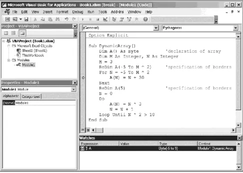
1.14. Manifestation of the error of real numbers’ computer representation 65 1.15. Arrays. . . 68
1.16. User-defined procedures . . . 77
1.17. Built-in procedures. Usage of standard windows. . . 85
1.18. Records . . . 90
1.19. Work with strings. . . 94
1.20. Work with text files. . . 101
1.21. Matrix terminology. Formulation of demonstration tasks . . . . 109
1.22. Program for transposing a matrix relative to its auxiliary diagonal . 111 1.23. User-defined forms . . . 116
1.24. Digression. Developing programs with the form in Microsoft Visual Studio. . . 129
Chapter 2. Programming in VBA . . . 133
2.1. Loading the form from the Excel window. Running the program executable file. . . 134
Contents
2.2. Layout of the control elements on the Excel worksheet . . . . 136
2.3. User-defined functions of Excel . . . 139
2.4. Two methods for developing Excel macros . . . 144
2.5. Excel Macro Recorder . . . 145
2.6. VBA code generated by Excel Macro Recorder and its editing . . . 148
2.7. Objects and events . . . 151
2.8. Object Application . . . . 154
2.9. Objects Workbook, Workbooks and ActiveWorkbook. . . . 161
2.10. Objects Worksheet, Worksheets and ActiveSheet . . . . 167
2.11. Objects Range, Selection and ActiveCell. . . . 171
2.12. Study of objects. . . 177
2.13. Using the Excel table as the user interface of programs . . . . 180
2.14. Two more Excel macros. Personal Macro Workbook . . . . 182
2.15. One more user-defined function of Excel. . . . 188
2.16. Digression. Change of Excel options . . . . 193
Chapter 3. Finite Difference Method for Solving Differential Equations. . . 195
3.1. Finite difference analogs of derivatives for a uniform grid. . . . 196
3.2. Finite difference scheme for the linear differential equation. The decomposition method . . . . 199
3.3. Sufficient stability conditions for the decomposition method . . . . 204
3.4. Simplification of the second-order linear differential equation. . . . 208
3.5. Program realization of the decomposition method . . . . 210
3.6. Examples of using the decomposition method . . . 212
3.7. Examples of the computing error. Instability and loss of accuracy. . 217 3.8. Solving the system of linear algebraic equations by using Excel functions . . . . . . . 223
3.9. Solving the system of linear algebraic equations by the Gaussian elimination method . . . 225
3.10. Two subroutines for solving the system of linear algebraic equations . . . 228
3.11. Reduction of the computing error. . . . 235
3.12. Solving the nonlinear differential equation by the quasilinearization method. . . . 238
3.13. Solving the Shockley-Poisson equation. . . . 241
3.14. Finite difference analogs of derivatives for a nonuniform grid. . . . 249
3.15. The decomposition method for a nonuniform grid . . . . 252
3.16. Solving the Shockley-Poisson equation on a nonuniform grid. . . . 255
3.18. The cyclic decomposition method . . . . 267
3.19. Program realization of the cyclic decomposition method . . . 271
3.20. Solving the oscillation equation. . . . 273
Chapter 4. Cubic Spline . . . . 281
4.1. Definition of cubic spline. Spline moments . . . 282
4.2. Spline interpolation . . . . 288
4.3. Use of cubic spline for processing transistor electrical characteristics . . . . 292
4.4. Spline integration . . . . 298
4.5. Iterative methods for solving the nonlinear algebraic equation. . . . 303
4.6. Noniterative method for solving the nonlinear algebraic equation. . 314
4.7. Calculating the charge storage capacity . . . 321
4.8. Subroutine for automatic creation of graphs . . . 327
4.9. Cubic spline usage for solving the second-order linear differential equation . . . . 329
4.10. Program realization of the cubic spline method for solving the linear differential equation . . . . 334
4.11. Solving the linear differential equation by the cubic spline method . 337 4.12. Modeling of heating of a geophysical cable. Locally one-dimensional scheme . . . . 340
Chapter 5. Quadratic and Linear Splines . . . . 352
5.1. Definition of quadratic spline. Spline slopes . . . . 353
5.2. Method for solving the initial value problem for the system of differential equations. . . 356
5.3. Program for solving the initial value problem . . . . 359
5.4. Solving the system of nonlinear algebraic equations by the Newton method. . . . 362
5.5. Newton and Newton-like methods for solving the single nonlinear algebraic equation . . . 365
5.6. Modeling of the piano mechanism linking a key with hammer. . . 372
5.7. Definition of linear spline. . . . 383
5.8. The least-squares method. . . 386
5.9. Program to determine the dependence of the wheat productivity on the land quality. . . . 390
5.10. The forward and backward Fourier transforms of a periodic function . . . 395
5.11. Subroutines for the forward and backward discrete Fourier transforms. . . 400
Contents
5.12. Solving the sound insulation problem . . . 406
Chapter 6. Numerical Methods for Nonlinear Programming . . . 415
6.1. Minimizing linear and nonlinear functions of several variables by the Solver add-in. . . . 417
6.2. Method for minimizing a nonlinear function of one variable. . . . . 428
6.3. The coordinate-descent method. . . . 432
6.4. Examples of using the minimization methods . . . . 437
6.5. The Powell minimization method. . . . 446
6.6. Determining the equilibrium state of a four-spring system. . . . 456
6.7. Minimization with nonlinear constraints . . . . 462
6.8. Minimization of the multimodal function. . . . 475
6.9. Minimization of the tabular function . . . . 483
6.10. Solving the nonlinear differential equation by the shooting method . 490 6.11. Modeling of the hammer motion in the piano mechanism . . . . 493
6.12. Nonlinear programming and the least-squares method. . . 501
Instead of Conclusions. . . . 510
Appendix 1. Data Types of Visual Basic and VBA . . . 513
Appendix 2. Greek and Russian Alphabets Denoted by Latin Letters. . . . 515
Appendix 3. The Main Mathematical Functions . . . 517
Appendix 4. Material for Tasks . . . . 518
Appendix 5. Analytical Method for Solving the Cubic Algebraic Equation . 520 Appendix 6. Realization of the Tangent Method by Using the Excel Circular Reference. . . 521
References List . . . 523
Introduction
Because of many advantages (above all, availability), tabular processor Excel, which is a part of Microsoft Office, is used in various areas of human activity: in economics and finances, electrical engineering and electronics, medicine, building construction, etc. This book is about Excel usage in applied mathematics.
While writing this book, the author pursued the following goals:
to teach the reader to program in the modern programming language, Visual Basic (VB), and its extension, Visual Basic for Applications (VBA);
on the basis of these programming languages, to give the reader full enough representation about numerical methods aimed at obtaining a solution of a task in the form of numbers (instead of formulas that are a result of using analytical methods);
to show that Excel with programs (macros), written by the reader in VBA, is convenient for solving applied tasks by numerical methods.
The book is intended for the reader familiar with Excel, Windows Explorer, Windows Clipboard and text editor Notepad for Windows. Besides, the reader should be conversant with higher mathematics and general physics. No prelimi-nary programming experience is necessary.
Learning this book is possible only by using a computer equipped with tabu-lar processor Excel.
According to the author’s opinion, there is no difference between terms “program” and “macro” when these terms concern the programming for Excel. Therefore, words “program” and “macro” are synonyms in this book.
The book contains six chapters, six appendices, a list of references and a sub-ject index.
In the first two chapters, we consider elements of Visual Basic Environment and main facilities of programming languages VB and VBA. The standard win-dow of operating system Winwin-dows, text file, user-defined form and Excel table are considered as the program user interface — the facility of dialogue between the user and program. We consider the creation of Excel user-defined functions. Besides, we demonstrate how to work with the program debugger, reference systems, Excel Macro Recorder and Personal Macro Workbook.
Introduction
In the third chapter, we consider the finite difference method for solving the second-order linear differential equation with two kinds of conditions on the solution, namely, the boundary and periodicity conditions. This is followed by a review of two versions of the decomposition method for solving systems of linear algebraic equations of special form called finite difference schemes. The simplest scheme is also solved by the Gaussian elimination method. The ques-tion of stability of the decomposiques-tion and Gaussian methods is investigated in respect of not increasing the computing error during solving the scheme. Using the Shockley-Poisson equation as an example, we consider the quasilinearization method for solving the nonlinear differential equation with boundary conditions. To demonstrate the possibilities of the finite difference method, we develop sub-routines and programs for solving mathematical and applied problems. We use the Excel scatter diagrams for visualization of calculation results.
Chapter 4 is devoted to the use of the third-degree (cubic) spline:
for interpolation, differentiation and integration of tabular (grid) func-tions;
for solving the nonlinear algebraic and linear differential equations. Besides, we consider:
two classical methods for solving the nonlinear algebraic equations, namely, the bisection and secant methods;
the locally one-dimensional scheme for solving the heat equation with two spatial coordinates.
We solve a series of applied problems to demonstrate the possibilities of the cubic spline construction. In addition to the macros and user-defined procedures (subroutines and function) realizing the numerical methods, a subroutine for automatic creation of graphs is developed.
In Chapter 5, we review the use of the second-degree (quadratic) spline for solving the initial value problem (of Cauchy) for the system of differential equa-tions. The first-degree (linear) spline is used in the least-squares method intended for determining parameters of a function. Besides, we review the following methods:
the Newton method for solving the system of nonlinear algebraic equa-tions;
the tangent, secant and Steffensen methods (called Newton-like methods) for solving a single nonlinear algebraic equation;
methods for the forward and backward discrete Fourier transforms of a periodic function.
Based on this theoretical material, we develop procedures and programs for solving applied problems.
Chapter 6 is mainly devoted to nonlinear programming, more precisely, to the question of finding the minimum of a nonlinear function of one or several
variables without calculating the function derivative or partial derivatives. This chapter begins with the use of the Solver add-in for Excel to minimize concrete linear and nonlinear functions of several variables. Further, we develop subrou-tines for finding the local minimum of a nonlinear function of general form, which are based on the coordinate-descent and Powell methods.
We review the following applications of the developed minimization subrou-tines:
for optimizing the size of a tin can;
for determining the equilibrium state of a four-spring mechanical system; for minimizing a nonlinear function with nonlinear constraints and a tabu-lar function of two variables;
for determining the local minima of a multimodal function of two varia-bles (with several local minima);
in the shooting method intended for solving the nonlinear differential equation with boundary conditions;
in the least-squares method.
Appendix 1 presents the data types of Visual Basic and VBA.
Appendix 2 contains the Greek alphabet with English names of the letters and the Russian alphabet denoted by Latin letters. The inclusion of this appendix is justified by the possible lack of Greek and Russian letters on the computer key-board. English names of Greek letters are used in texts of program modules and source data for programs. Russian letters in Latin are mainly used in the refer-ences list.
Appendix 3 contains the main mathematical functions of Visual Basic. In ad-dition, this appendix contains operators allowing the use of mathematical func-tions not included in the programming language.
Appendix 4 contains data for tasks intended to consolidate the book material and check up its understanding.
Appendix 5 presents an analytical method for solving the cubic algebraic equation. We use this method in Chapter 4.
Appendix 6 demonstrates the use of circular reference in Excel for solving the nonlinear algebraic equation by the tangent method.
The subject index contains the main terms and designations with numbers of pages, on which their sense is uncovered. It will allow using the book as a reference manual.
The present book is based on author’s books [1, 2] approved by the Scientific and methodical council in computer science at the Ministry of Education and Science of the Russian Federation as a manual on discipline “Computer science” for university students.
In the book, we often speak about mathematical (computer, numerical) modeling. The essence of mathematical modeling lies in the replacement of
Introduction
an object, in particular of a process, by an appropriate mathematical model and in its further study by using a computer. Operation with the model, instead of the object, allows to obtain operatively detailed information, showing internal con-nections of the object and its qualitative and quantitative characteristics. The mathematical modeling is so popular that, when speaking about it, adjective “mathematical” may be omitted, as in this book.
In writing the book, we used a personal computer equipped with 32-bit version of the Windows 7 operating system and Microsoft Office Professional Plus 2013 Preview. For obtaining information, shown in Fig. 1.8, 2.23 and 3.6, the reference system of Excel 2010 was used. The system disk name is C and the computer user name is usr in the book.
We will need the Developer tab in Excel Ribbon (a part of the Excel win-dow), among tabs Home, Insert, Page Layout, etc. If such a tab does not exist, we fulfill the following:
1) click on the File button in the top left corner of the Excel window (in Excel 2007, click on the Office button);
2) click on the Options button;
3) in the Excel Options window opened, click on button Customize Ribbon; 4) in area Customize the Ribbon:
set Main Tabs by using the drop-down list; then turn on option Developer;
5) click on the OK button.
This operational sequence can be written as the following formula: File > Options > Customize Ribbon > Main Tabs > turn on Developer > OK. We will frequently use such formulas.
When opening an Excel workbook containing a macro, the Security Warning panel can appear. To allow the macro to work, we must click on the Enable Content button of this panel.
When executing a macro, cycling is possible. To interrupt it, we must press the Esc key on the computer keyboard.
The enclosed compact disk (CD) contains text files with program modules and with source data for programs. The texts on the CD correspond to the num-bered listings in the book. A method of work with these files is described on pp. 26 and 245.
The program texts on the CD may be used as templates when developing programs for solving other tasks with the same mathematical formulation as the tasks considered in the book.
For contact with the author, the following internet resources can be used: [email protected], http://gzgarber.narod.ru/.
Chapter 1.
Programming in Visual Basic
We review elements of Visual Basic Environment, a part of Microsoft Office, and constructs of the Visual Basic programming language. The standard window of operating system Windows, text file and form are used as the user interface of programs.
In addition, we demonstrate how to work with the program debugger and reference systems.
1.1. Elements of Visual Basic Environment
1.1. Elements of Visual Basic Environment
For writing and debugging programs, we will use Visual Basic Environment, which is a part of Microsoft Office.
Program debugging involves detection and correction of errors that, as a rule, are present in a program text just written.
To go to Visual Basic Environment, we must fulfill the following two opera-tions:
1) in the Excel window (with the active workbook by name Book1), activate the Developer tab by clicking on it;
2) click on the Visual Basic button in area Code.
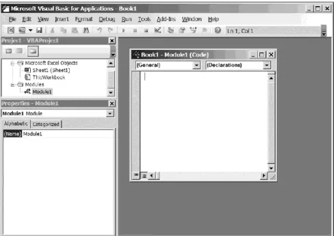
As a result, the Visual Basic Environment window is displayed (Fig. 1.1). In this window, we can perform various actions: entering and editing the pro-gram text, as well as debugging and executing the propro-gram. Further, we will use a shorter name for this window and call it “the VB window”.
The program is also called an application or project. It will be in the Excel workbook (by name Book1).
Let us consider the elements of the VB window.
1. Menu bar. There are standard menus, like in many windows of the operating system: File, Edit, View, Tools and Help. The Insert menu is used for organizing a place for program storage (in the workbook). Menus Debug and Run are respectively used for debugging and running the program.
2. Context menu. It serves for convenience of work in the area (of the VB window), in which the mouse pointer is located.
For using the context menu:
1) place the mouse pointer in the necessary area of the screen and make the right click;
2) click (by the left mouse button) on the required command of the displayed menu.
3. Toolbars: Standard, Edit, Debug and others. Only the standard toolbar is displayed by default. To add or remove any toolbar, we have to fulfill View > Toolbars and to click on the required command of the displayed menu. The check (tick) mark against the command testifies to the presence of the corre-sponding toolbar on the display screen.
Fig. 1.1. The Visual Basic Environment window including the standard toolbar, the project explorer window and the properties window Let us consider the toolbars.
1. Toolbar Standard is displayed by default. It allows us to perform a wide spectrum of actions.
This toolbar is usually located under the menu bar, however, we can move it to other areas of the VB window by using the mouse.
2. Toolbar Edit is intended for work with the program text. It realizes possi-bilities of an elementary text editor:
copying and moving a text fragment to Windows Clipboard; inserting the text fragment from Windows Clipboard; search and replacement of words and phrases, etc.
3. Toolbar Debug is intended for debugging the program. Many provisions are made for debugging:
observation of the current values of the program variables;
step-by-step program execution, in which one operator (statement, in-struction) or its part is performed on each step, etc.
1.1. Elements of Visual Basic Environment
As a rule, we will review programs without a user-defined form as the program user interface. Development of such program begins with inserting a module into the active Excel workbook. For inserting a module, let us fulfill the following sequence of operations.
1. In the Excel window, Developer > Visual Basic in area Code. As a result, the VB window appears, including the project explorer window and the proper-ties window (Fig. 1.1).
If the project explorer window is not displayed, we have to click on Project Explorer in the View menu. We will need the properties window only in Section 1.23.
2. Select line VBAProject (Book1) by clicking on it in the project explorer window.
3. Insert > Module.
As a result, a line corresponding to the inserted module, Module1, appears in the project explorer window. Besides, an empty window opens; it is the code window corresponding to Module1 (Fig. 1.2). In this window, we will create the program text by using the computer keyboard.
Fig. 1.2. The VB window, including the code window, after inserting Module1 into the Excel workbook
For opening the code window corresponding to the module inserted earlier, we have to click twice on the name of this module in the project explorer window.
To delete a module:
1) make the right click on the module name (for example Module1) in the project explorer window;
2) in the context menu opened, click on the Remove command;
3) click on the No button in the open window with a question about export-ing the module before removexport-ing it.
Before the computer will execute a program, we (as the program developer) must form its text in the code window. The first and last lines (operators) of the program are standard:
Sub name() End Sub
On p. 79, we will consider the origin of word Sub. Word name means the program name appointed by us.
The name must satisfy the following conditions: the first character should be a letter;
the name must include only letters, figures and the underscore character; the name must include less than 256 characters.
As we see, the name cannot include the space character. To use name consisting of several words, we have:
to begin each word with a capital (uppercase) letter;
to use the underscore character instead of the space character. Examples of the program name follow:
MyProgram13 my_program MyProgram_13
Between the first and last lines of the program, we have to place other lines (operators) of this program. For that, it is possible to use Windows Clipboard and habitual commands of editing (as in Notepad). After typing a new line, we have to press the Enter key on the keyboard.
Let us start with a simple program based on the Pythagoras theorem,
2 2
b a
c , (1.1) for calculating length c of the hypotenuse of a right-angled triangle with legs a = 3 and b = 4.
1.1. Elements of Visual Basic Environment
In the code window, we type the following program text (Fig. 1.3): Sub Pythagoras()
a = 3 b = 4
c = Sqr(a ^ 2 + b ^ 2) End Sub
In this text, Pythagoras is the program name, a, b and c are names of varia-bles, Sub is a keyword, EndSub is a keyword combination. The program and variable names are appointed by us.
Fig. 1.3. The VB window with the Pythagoras program in the code window In a programming language, words used only in the language constructs are called keywords. We cannot use keywords as names of programs and variables in programs. By default, Visual Basic Environment is tuned in such manner that all keywords are highlighted in blue color (at formation of the program text in the code window), comments are highlighted in green, syntactic errors — in red.
It is visible that the power operation (^) is written as in Excel, Sqr is the square root function (in Excel, the square root function is SQRT).
For convenience, if we need to place an operator on several lines, for carry-ing over, we have to type the space character with the subsequent underscore character. At the finish of typing these characters, we have to press the Enter key on the keyboard.
If we need to place several operators on one line, we have to type a colon between these operators.
An apostrophe means that information following it (up to the line end) is a comment, i.e., a character set, which does not influence the program execution.
Thus, our program can be written as follows: Sub Pythagoras()
a = 3: b = 4 c = _
Sqr(a ^ 2 + b ^ 2) 'according to Pythagoras End Sub
If a comment occupies several lines, each line must be preceded by an apos-trophe. For example, program
Sub Pythagoras() a = 3: b = 4
c = Sqr(a ^ 2 + b ^ 2) 'according to Pythagoras: 'pythagorean pants are 'equal in all directions End Sub
is equivalent to the previous program.
To save the program, we fulfill the following: 1) in the Excel window, File > Save As > Browse;
2) in the Save As window opened, choose a folder intended for saving the Excel workbook, for example, My Documents;
3) by means of drop-down list Save as type, set the following file type: Excel Macro-Enabled Workbook;
4) click on the Save button.
As a result, the Pythagoras program is saved as a part of the Excel work-book by name Book1 with extension .xlsm.
For returning to the Pythagoras program: 1) open the Book1 workbook;
2) if the Security Warning panel appears, click on button Enable Content; 3) go to Visual Basic Environment;
4) click twice on Module1 in the project explorer window. We will execute the Pythagoras program in the next section.
1.2. Main commands of the program debugger
1.2. Main commands of the program debugger
After typing the program text, the detection and correction of errors in the program follows. At this stage, we can use the debugger.
Let us consider the main commands of the debugger; we can see them in the Debug menu of the VB window.
1. Step Into — the execution of one program operator or its part. The click on Step Into is equivalent to pressing the F8 key on the keyboard. This command is used for the step-by-step program execution.
2. Run To Cursor — the execution of the program up to the blinking cursor. The click on Run To Cursor is equivalent to pressing Ctrl + F8.
For setting the blinking cursor in the proper place of the program, we have to click on this place.
If we speak about key presses, the plus sign means the synchronism of these presses, i.e., “pressing Ctrl + F8” means “simultaneous pressing the Ctrl and F8 keys”.
3. Toggle Breakpoint — the installation or liquidation of the breakpoint at the place, where the blinking cursor is located. The breakpoint marks the pro-gram line, where the propro-gram execution stops. This command can also be per-formed by pressing the F9 key.
For the installation or liquidation of the breakpoint, we can click on the left border of the code window against the proper line.
4. Clear All Breakpoints — the liquidation of all breakpoints. This com-mand can also be performed by pressing Ctrl + Shift + F9.
5. Add Watch — the current visualization of the value of a variable. We will review the command usage in Section 1.15.
In addition to commands Step Into and Run To Cursor, two more commands for the program execution, Step Over and Step Out, are in the Debug menu. We will review them in Section 1.16.
Let us consider commands Run and Reset located in the Run menu of the VB window.
1. Run — the start of the program execution (or shorter, of the program) and transition from one breakpoint to another. If the breakpoints are absent, the pro-gram is executed completely. This command is represented by arrow ► on the toolbars of the VB window, in particular, on the standard toolbar.
The program can be started from the Excel window; we will consider this possibility later (p. 113).
2. Reset — the discontinuation of the program execution. This command is represented by square
■
on the toolbars.During the program execution stops (in particular, at the breakpoints), yellow color highlights the operator, which is not executed yet. If we place the mouse pointer on a variable, its value is displayed.
For obtaining the hypotenuse length by means of the Pythagoras program from the previous section, we fulfill the following:
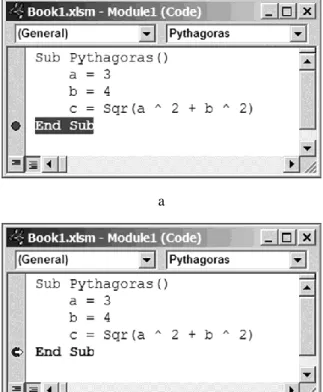
1) click on the left border of the code window against the last line of the program for marking this line by the breakpoint (Fig. 1.4a);
2) click on arrow ► for executing the Pythagoras program up to the breakpoint;
3) if window Macros appears, successively click on the Pythagoras line and the Run button in this window;
4) in the code window, whose state is depicted in Fig. 1.4b, place the mouse pointer on the c variable in the program text; c = 5 appears (Fig. 1.5);
5) click on arrow ► for terminating the program execution.
After starting the program execution, a window containing message Can’t execute code in break mode may appear, indicating that we forgot to terminate (or to discontinue) the previous program execution. For correcting this error, we fulfill the following:
1) click on the OK button in the message window;
2) click on arrow ► (or on square
■
) for termination (or discontinuation) of the program execution;3) restart the program.
The program execution means consecutive execution of its operators: at first, the computer sets the values of variables a and b, and then calculates the value of c. To be convinced, we have to liquidate the breakpoint (by clicking on it) and to execute the Pythagoras program step-by-step by the F8 key, watching the change in variables a, b and c.
Let us assume that an error was committed: when typing operator c = Sqr(a ^ 2 + b ^ 2)
we pressed the minus key on the keyboard instead of the plus key. In this case, the program execution stops, and a window appears with the following message: Run-time error ‘5’: Invalid procedure call or argument.
To understand our error, we click on button Debug in the message window. As a result, the place, where the stop occurred, is highlighted in yellow color. Looking at the values of a and b, we can understand the reason of the stop — the negative value of the argument of the square root function.
1.2. Main commands of the program debugger
a
b
Fig. 1.4. The Pythagoras program with the breakpoint (a) before and (b) after starting the program execution
For fuller information on the possible reasons of the stop, we fulfill the fol-lowing:
1) remaining in Visual Basic Environment, start the Excel help system by pressing the F1 key;
2) type Error 5 in the text box of the Excel Help window; 3) click on the Search button;
4) click on the following line of the open list: Invalid procedure call or argument (Error 5).
After correcting our error (that is, after changing minus to plus), we have to restart the program.
During the execution, our program (as a set of zeros and units) is located in the main memory of the computer. This program is being executed by the pro-cessor that performs different operations including, among others, arithmetic operations.
1.3. Variables. Data types
1.3. Variables. Data types
Variables in programming have about the same meaning as variables in algebra. We recommend declaring a variable before its usage.
The declaration operator has the following syntax: Dim variable [As type]
In this language construct:
Dim (from “dimension”) is the keyword testifying the appearance of a new variable;
variable is the variable name; As is the keyword;
type is the data type (Appendix 1) of the declared variable.
Here and below, the square brackets indicate an optional part of the syntax, i.e., the part that may be absent. Such usage of the brackets is acceptable because the square and curly brackets are not used in constructs of Visual Basic.
In other words, the declaration operator has the following two versions: Dim variable As type
Dim variable
Initially, we will consider the first version.
When (during the program execution) the computer meets the Dim operator, it allots a memory cell for the variable by name variable. The cell size (in bytes) is defined by type — the data type of the variable; type is keyword Boolean, Byte, Integer, Long, Currency or so on (Appendix 1).
According to the second column of the table in Appendix 1, the memory cell sizes, corresponding to different variables, can strongly differ.
To understand how much information is contained in one byte, let us notice that three bytes are usually enough for storing information on one pixel (the color point on the display screen) — one byte each for intensities of the red, green and blue colors.
One Dim operator allows declaring several variables if we list them through a comma. The example operators follow:
Dim my_variable As Double
Dim i As Byte, j As Integer, k As Integer
The restrictions on names of variables are the same as on names of programs (p. 16), at that, the upper or lower case of letters does not matter. For example, if the Alpha variable is declared and we try to declare the alpha variable, Alpha will be automatically replaced by alpha.
Alpha is the English name of a Greek letter. If the keyboard does not support the Greek language, we recommend to use English names of Greek letters according to Appendix 2 when naming variables and programs.
For reducing programming errors, we recommend to tune Visual Basic Envi-ronment so that it demands the declaration of variables. For this purpose, we fulfill the following:
1) open menu Tools in the VB window; 2) click on Options;
3) activate the Editor tab;
4) turn on option Require Variable Declaration; 5) click on the OK button.
As a result, the code window corresponding to a new module will contain the following first line:
Option Explicit
We can also put this line into the code window (or remove it) manually, as a usual program line.
In the presence of line OptionExplicit, the computer diagnoses the use of an undeclared variable in the program text: during the program execution, the computer displays message Variable not defined.
Data types Byte, Integer, Long, Currency, Single and Double (Appendix 1) are called numerical data types.
According to the third column of the table in Appendix 1:
in a memory cell, corresponding to a variable of the Byte data type, non-negative integers (up to 255) can only be stored;
in a cell, corresponding to a variable of the Integer or Long data type, integers can be stored;
in a cell, corresponding to a variable of the Currency, Single or Double data type, decimal numbers can be stored.
Let us pass to the second version of the Dim operator (p. 23).
If we do not specify the data type when declaring a variable (for example, by operator DimW), the variable (by name W) automatically receives the Variant data type. It means that any information can be stored in a memory cell,
corre-1.3. Variables. Data types
sponding to this variable; i.e., the Variant data type is similar to the general format of Excel.
Let us consider operator Dim i, j As Integer
This operator is equivalent to the following: Dim i As Variant, j As Integer
If we need the Integer data type for both variables, i and j, we should declare them as follows:
Dim i As Integer, j As Integer or
Dim i As Integer Dim j As Integer
Later we will consider ways of declaring variables without the use of the Dim keyword (p. 81).
As an example of using the declaration operator, let us consider the following program for calculating the number of days in the 20th century and defining the current date and time:
Listing 1.1 Sub Century_20()
Dim D1 As Date, D2 As Date, D3 As Date Dim N As Long
D1 = #1 Jan 1900# 'beginning date of century D2 = #31 Dec 1999# 'ending date of century N = D2 - D1 + 1 'number of days in century D1 = Time 'current time
D2 = Date 'current date D3 = Now 'date and time End Sub
In the second and third lines of this program, Date and Long are the data types (Appendix 1); #1Jan1900# and #31Dec1999# mean dates on Janu-ary 1, 1900 and December 31, 1999. The subtraction of the first date from the second date determines the number of days between these dates.
Word Time means determination of the current time by means of the VB function by name Time. In other words:
Time is the call of the Time function of VB;
the value of this function is the current time of the day or, that is the same, the Time function returns the current time of the day into the program (“into the program” may be omitted).
In operator D2 = Date
word Date means the call of the Date function returning the current date into the program.
We see that Date is a name of the VB function and a name of the data type. Thanks to various contexts, it does not lead to confusion.
Word Now means the call of the Now function returning the current date and time together.
Regarding the VB functions, we will talk in more details later, in particular, in Sections 1.4 and 1.9.
To be convinced of the operational capability of the Century_20 program, we fulfill the following operations:
1) insert a module into the active Excel workbook (p. 15);
2) enter the Century_20 program text into the code window of the new module;
3) make the step-by-step execution of this program by means of the F8 key, watching the values of variables D1, D2, D3 and N.
It should be emphasized that, before the first press of key F8, we must place the blinking cursor inside the program text, not in line OptionExplicit.
Text Listing 1.1 of the Century_20 program can be entered into the code window by means of the keyboard. We can also copy it from the enclosed CD.
For copying:
1) open file Listing_1_01.txt with the Notepad editor, for example, by dou-ble click on the pictogram of this file in Windows Explorer;
2) in the Notepad window opened, highlight the program text and copy it into Windows Clipboard, for example, by pressing Ctrl + C;
3) by the click, locate the blinking cursor in the code window of Visual Basic Environment;
4) paste the program text from Windows Clipboard into the code window, for example, by pressing Ctrl + V;
1.4. Two main functions for conversion of data types
1.4. Two main functions for conversion of data types
A string is a quoted sequence of characters. The example strings follow: "Hello, World!"
"13.333" "37 RUR" "$ 37" " "
The last string contains only the space character.
Let us supplement the string definition by the empty string, "", which does not contain any characters.
Strings " " and "" are used in program Listing 1.7. In Section 1.19, we will expand the string definition even more.
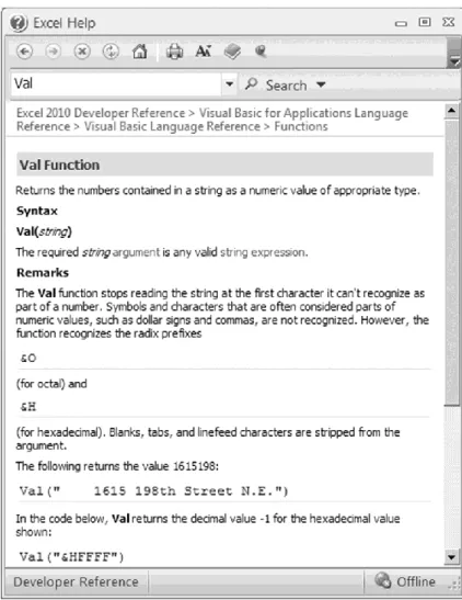
Converting string to number is often necessary. For this purpose, the Val function is used. It converts the numerical beginning of string to number. If the Val function cannot perform this, it returns zero into the program. The argument of the Val function is a string; this function returns a number.
For the backward conversion (that is, number to string), the Str function is used. The argument of this function is a number, variable of numerical data type (p. 24) or arithmetic expression (Section 1.8). The Str function returns a string.
Let us make the step-by-step execution of the program below.
Listing 1.2 Sub StrVal()
Dim strA As String Dim curB As Currency strA = "45.77"
curB = Val(strA) 'result: curB = 45.77 strA = Str(curB) 'result: strA = " 45.77" curB = Val("4.7 = X") 'result: curB = 4.7 curB = Val("4,7 = X") 'result: curB = 4 curB = Val("X = 4.7") 'result: curB = 0 curB = Val("") 'result: curB = 0 End Sub
The first comment corresponds to the case when operator strA = Str(curB)
is highlighted in yellow color during the step-by-step program execution. This comment means the following: if the mouse pointer is located on curB, infor-mation curB = 45.77 appears.
Information curB = 45.77 is the result of executing operator curB = Val(strA)
which is in the same line with the comment.
The second comment corresponds to the case when operator curB = Val("4.7 = X")
is highlighted in yellow color during the step-by-step execution. This comment means the following: if the mouse pointer is located on strA, information strA = “ 45.77” appears. And so on.
All comments, which begin with word “result” or “Returns” (p. 33), have similar sense.
Let us remind that, during the stops of the program execution, yellow color highlights the operator, which is not executed yet.
In addition to the Val and Str functions, there are other functions for con-version of data types. We will review them in Section 1.8.
1.5. Constants
1.5. Constants
Constants are similar to variables. However, unlike a variable, the content of the memory cell, corresponding to a constant, cannot be changed during the pro-gram execution. There are two versions of constants in Visual Basic, named built-in and user-defined constants.
The user-defined constant can be declared by means of operator Const invariable [As type] = value
In this operator:
Const is the keyword testifying the appearance of a new constant; invariable is the constant name;
As is the keyword, as in the Dim operator (p. 23);
type is the data type (Appendix 1) of the declared constant; value is a value of the declared constant.
The restrictions on names of constants are the same as on names of variables and programs (p. 16).
Examples of the constant declaration follow: Const e As Double = 2.718281828
'base of natural logarithm Const e = 2.718281828
Const phi = 1.618033989 'gold relation Const Flag As Boolean = False
Const Message = "End of Work"
Const Millennium As Date = #1 Jan 2000# Const beta As Currency = 2 ^ 0.5
In the fourth example operator, Boolean is the so-called logical data type (Appendix 1).
When executing the last operator, the rounded square root of 2 (that is, 1.4142) is assigned to constant beta. This example shows that value in the Const operator can be an elementary arithmetic or logical expression
(Sec-tions 1.8 and 1.10). In this case, the content of the memory cell, corresponding to the constant, is determined by the expression value rounded according to the type data type.
One Const operator allows declaring several constants if we list them through a comma. The example operator follows:
Const Min = 0, Max = 1000, tau As Double = 6.283185307 As an example of using constants, let us consider the following program for conversion of an angle from degrees to radians:
Sub deg2rad()
Dim angleD As Double Dim angleR As Double
Const pi As Double = 3.141592654 'pi = tau / 2 angleD = 270 'angle equals 270 degrees angleR = angleD * pi / 180
'result: angle in radians End Sub
As we see, operator
Const pi As Double = 3.141592654 declares the pi constant before its usage in operator angleR = angleD * pi / 180
The rad2deg program below, which converts an angle from radians to degrees, is similar to the above program.
Sub rad2deg()
Dim angleD As Double Dim angleR As Double
Const pi180 As Double = 3.141592654 / 180
angleR = 4.5 'angle equals 4.5 radians angleD = angleR / pi180
'result: angle in degrees End Sub
On p. 82, we will consider the declaration of a constant by means of keyword combination PublicConst.
1.5. Constants
The built-in constant does not need any declaration. Names of the built-in constants of Visual Basic begin with prefix vb, for example, vbFriday (this con-stant equals 6).
For names (in particular, names of constants), the developers of Windows accepted the following agreement: names of similar data begin with the same short prefix. In particular, the built-in constants of Visual Basic have prefix vb, the built-in constants of Excel have prefix xl.
In addition to vbFriday, we will come across the following built-in constants: vbYesNo, vbYes, vbTab, vbCrLf, vbCr, vbLf, xlR1C1, xlCalculationAutomatic, xlCalculationManual, xlDialogOpen, xlDialogSaveAs, xlCenter, etc.
1.6. Obtaining information
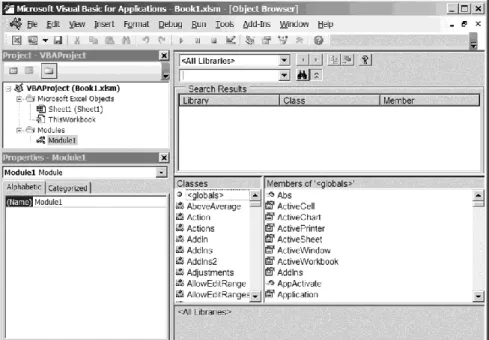
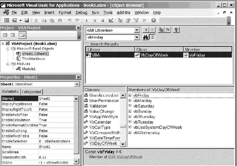
For obtaining information on a built-in constant, we must press the F2 key when the VB window is active. As a result, the object browser window appears (Fig. 1.6). In the top box of this window, we should set <All Libraries> by means of the drop-down list. In the text box below, we should type what is interesting for us, for example, vbFriday. Then we click on the binoculars picto-gram. The answer is in the Search Results area (Fig. 1.7).
For closing the object browser window, we have to click on the little cross at the right end of the menu bar.
Fig. 1.6. The VB window with the object browser window instead of the code window
1.6. Obtaining information
Fig. 1.7. Information on the built-in vbFriday constant
The Excel help system, started by pressing the F1 key, is useful too (p. 22). For accelerating the process of finding the necessary information, the blinking cursor must be preliminarily located on the word of interest.
By means of the Excel help system, we will study the Val function. For this purpose, let us fulfill the following.
1. Enter the StrVal program (p. 27) into the code window. 2. Locate the blinking cursor on the Val word by clicking on it.
3. Press the F1 key. As a result, the Excel Help window, containing the full information on the Val function, is displayed (Fig. 1.8).
4. After studying the last information, copy fragment Dim MyValue
MyValue = Val("2457") ' Returns 2457. MyValue = Val(" 2 45 7") ' Returns 2457. MyValue = Val("24 and 57") ' Returns 24.
from the bottom part of the Excel Help window into the StrVal program as follows:
1) highlight this fragment by the mouse, as in Notepad; 2) copy it into Windows Clipboard by pressing Ctrl + C;
3) locate the blinking cursor in the code window, against the last line of the StrVal program;
4) paste the fragment from Windows Clipboard into the program text by pressing Ctrl + V.
1.6. Obtaining information
As a result, the StrVal program takes the following form: Sub StrVal()
Dim strA As String Dim curB As Currency strA = "45.77"
curB = Val(strA) 'result: curB = 45.77 strA = Str(curB) 'result: strA = " 45.77" curB = Val("4.7 = X") 'result: curB = 4.7 curB = Val("4,7 = X") 'result: curB = 4 curB = Val("X = 4.7") 'result: curB = 0 curB = Val("") 'result: curB = 0 Dim MyValue
MyValue = Val("2457") ' Returns 2457. MyValue = Val(" 2 45 7") ' Returns 2457. MyValue = Val("24 and 57") ' Returns 24. End Sub
We advise the reader to execute this program step-by-step (by means of the F8 key), watching the value of the MyValue variable.
1.7. Assignment operator
The assignment operator has the following syntax: variable = expression
Here, variable is the variable name, expression is an arithmetic or logical expression (Sections 1.8 and 1.10) or string, which can be considered as an expression (Section 1.19). A separately taken number, constant, variable or func-tion is also an arithmetic expression. In the assignment operator, = is the so-called assignment sign.
The assignment operator works as follows: 1) the value of expression is calculated;
2) the resulting value is assigned to variable, i.e., is written into the cor-responding memory cell.
If the data type of the variable in the left-hand side of the assignment operator does not coincide with the type of the expression value in the right-hand side, the value type is generally converted (transformed) during the execution of the assignment operator.
Let us make the step-by-step execution of the following program for convert-ing strconvert-ings "78.8", "78,8" and "78;8" to numbers of the Currency data type.
Sub Conversion()
Dim curA As Currency Dim curB As Currency Dim curC As Currency
curA = "78.8" 'result: curA = 78.8 curB = "78,8" 'result: curB = 78.8 curC = "78;8" 'result is absent End Sub
Because of executing the first and second assignment operators, strings "78.8" and "78,8" are successfully converted to number 78.8.
1.7. Assignment operator
curC = "78;8"
the stop occurs with the following information: Run-time error ‘13’: Type mis-match. It speaks about the following:
the types of variable on the left and of value on the right of the assign-ment sign (=) are different;
the computer cannot convert string "78;8" to a number.
We will continue considering the data type conversion in the next section of the book.
Unlike other programming languages, for example C++, multiple assign-ments, for example x=y=z=1.3, are inadmissible in VB. We have to use several assignment operators with the same right-hand side, i.e., language con-struct x = 1.3 y = 1.3 z = 1.3 or x = 1.3: y = 1.3: z = 1.3 is correct.
1.8. Arithmetic expression
In Visual Basic, an integer is represented by a sequence of figures with the minus sign or without any sign. Examples of integers are
–18 32 0
If a number has the fractional part, it separates from the integral part by a point. In this case, we may omit the integral part if it equals zero. Examples of decimal numbers follow:
0.5 –5.68 –.12 .035 3.
In the last example, 3 with a point means a number with zero fractional part, i.e., an integer, in fact.
We reviewed the main form of decimal numbers.
Decimal numbers may also be represented in exponential form. For example, -1.6E-19 is the electron charge, -1.6·10-19C (its absolute value figures in
Sec-tion 3.13). Instead of E, letter D may be used in the exponential representaSec-tion, i.e., the electron charge, -1.6·10-19C, may be written as -1.6D-19
One of the main constructs of any programming language is an arithmetic expression similar to the algebraic expression in mathematics. However, we can-not omit the multiplication sign in the arithmetic expression. Table 1 below con-tains equivalent algebraic and arithmetic expressions.
Table 1. Examples of expressions
Algebraic expression Arithmetic expression of VB
y x 12 5 5 * x + 12 * y y x x / y x y y ^ x x x 19.55·10-6 19.55E-6 or 19.55D-6
1.8. Arithmetic expression
The arithmetic expression contains the invariables (numbers and constants), variables and/or functions related by arithmetic operations. As we already men-tioned in the previous section, an individual number, constant, variable or func-tion is also an arithmetic expression.
The expressions in Table 1 do not include functions. We will review arithme-tic expressions with functions in the next section.
Arithmetic operations are denoted as follows: + (addition), - (subtraction or sign change operation), * (multiplication), / (division), ^ (power operation), \ (integer division, i.e., division of integers neglecting the integer remainder), Mod (modulus operation, i.e., determining the integer remainder after division of integers).
According to the assignment operator syntax, the arithmetic expression is on the right of sign =. For example, assignment operator
z = 5 * x + 12 * y includes arithmetic expression 5 * x + 12 * y
Let us consider the following program: Sub Arithmetic1() Dim m As Integer Dim n As Integer Dim x As Double m = 5 n = 2 x = m / n 'result: x = 2.5 x = m \ n 'result: x = 2 x = m Mod n 'result: x = 1 End Sub
To verify the correctness of this program, we advise the reader to make the step-by-step execution (by means of the F8 key), watching the change in the value of x.
If the arithmetic expression contains several operations, the order of their per-formance is defined by the following rules of priorities of arithmetic operations:
1) first of all, the power operation (^) is performed;
2) next, the multiplication and division (*, /) are performed in that sequence as they are in the expression;
3) the integer division ( \ ); 4) the modulus operation (Mod); 5) the sign change operation (–);
6) finally, the addition and subtraction (+, –) are performed in that sequence as they are in the expression.
As we see, the power operation (^) has the highest priority in VB.
The rules of priorities of arithmetic operations in VB differ from the rules of priorities in Excel regarding the power operation, multiplication, division, the sign change operation (so-called negation), addition and subtraction: the nega-tion (–) is performed first, i.e., has the highest priority in Excel.
To be convinced, we put =-1^2
into the Excel formula box and click on the tick button of the Excel formula bar (or press the Enter key). As a result, value 1 appears in the active cell on the worksheet. After the execution of VB operators
Dim i As Integer i = -1 ^ 2
the i variable is equal to -1.
In both VB and Excel, parentheses are used for changing the sequence of the operations: the values of the parenthesized arithmetic expressions are calculated at first.
We will not see the square and curly brackets in the arithmetic expressions of Table 2 below because, as it was already told, such brackets are not used in the VB constructs.
When calculating the expression value, results of performance of intermedi-ate arithmetic operations remain in the processor or are written into cells of the cache memory (from where they are read when required).
The cache memory has a short time of reference (that is, of writing and read-ing information); this time is much shorter than the time of reference for the main memory. The cache memory is intended for temporary storage of interme-diate results and contents of memory cells often used. The program fragment, which is being executed, may also be stored in the cache memory.
Let us consider the following assignment operator with the arithmetic expres-sion in the right-hand side:
z = 5 * x + 12 * y
1.8. Arithmetic expression
1) multiplies 5 by the content of cell x;
2) writes the result into a cache memory cell, for example, cache1; 3) multiplies 12 by the content of cell y;
4) adds the result to the value of cache1; 5) writes the result into cell z.
Table 2. Examples of expressions Algebraic
expression Arithmetic expression of VB
7{3[a+b(c+d)]+8}+2 7 * (3 * (a + b * (c + d)) + 8) + 2 -ab -a ^ b or –(a ^ b) a-b a ^ (-b) ab-c a ^ (b - c) 10-4.7 10 ^ (-4.7) 104.7 10 ^ 4.7 A·B A * B A(-B) A * (-B) -A * B or -(A * B) c b a a ^ (b ^ c) c b a ) ( a ^ b ^ c or (a ^ b) ^ c d c b a (a * b) / (c * d) or a * b / (c * d) a·104 a * 1E4 a * 10E3 or a * 10000
In mathematics and programming, participants of operations are called operands, both in the case of arithmetic operations and in the case of logical operations (Section 1.10). For example, arithmetic expression 5*x includes the following two operands: integer 5 and variable x.
For a better understanding of the rules of priorities of arithmetic operations, let us consider the following program:
Sub Arithmetic2() Dim m As Integer Dim n As Integer Dim x As Single Dim y As Single x = 3 m = 2 n = -1 y = (-3) ^ m 'result: y = 9 y = -(3 ^ m) 'result: y = -9 y = -3 ^ m 'result: y = -9 y = 10 + (x + 7) ^ (m + n) 'result: y = 20 y = 10 + x + 7 ^ m + n 'result: y = 61 End Sub
We advise the reader to make the step-by-step execution of this program, watching the value of the y variable and explaining the value origin.
In addition, we advise the reader to verify that (m \ n) * n + m Mod n
equals m for arbitrary integers m and n (naturally, n ≠ 0). For that, the reader has to write a program, which is similar to Arithmetic1, and to execute the new program step-by-step.
Arithmetic expressions may contain variables and invariables of different types. If the type of the value of arithmetic expression in the right-hand side of the assignment operator (on the right of sign =) does not coincide with the data type of the variable in the left-hand side of the assignment operator (on the left of sign =), the type of the value is converted during the assignment.
Let us consider the situation when the value of arithmetic expression on the right of sign = has a fractional part and the variable on the left of sign = is of the Integer or Long data type. During the assignment, the value is transformed according to the following rules for rounding off:
if the fractional part of the value is equal to 0.5, this value is rounded up to the even number from two nearest integers;
otherwise, the value is rounded up to the nearest integer.
Because operations \ and Mod are applicable only to integers, the execution of these operations over numbers with a fractional part begins with the rounding
1.8. Arithmetic expression
off the operands to integers according to the formulated rules. The results of operations \ and Mod are integers.
An operation with one operand is called a unary operation. Among the arith-metic operations, only the sign change operation (–) is unary. An operation with two operands (^, *, /, \, Mod, +, – as subtraction) is called a binary operation.
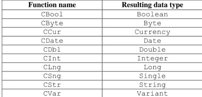
VB includes special functions for converting data types. Two of these func-tions (Str and Val) were reviewed in Section 1.4; the remaining funcfunc-tions are listed in Table 3 below.
Table 3. Functions for converting data types
Function name Resulting data type
CBool Boolean CByte Byte CCur Currency CDate Date CDbl Double CInt Integer CLng Long CSng Single CStr String CVar Variant
Requirements to the argument of these functions and examples of their usage are given in the Excel help system. For accelerating the process of finding the necessary information, we must press the F1 key when the VB window is active.
Let us make the step-by-step execution of the program below. Sub Functions()
Dim intN As Integer Dim strN As String Dim curN As Currency intN = -15 strN = Str(intN) 'result: strN = "-15" strN = CStr(intN) 'result: strN = "-15" intN = 15 '8th operator strN = Str(intN) '9th operator 'result: strN = " 15" strN = CStr(intN) '10th operator 'result: strN = "15" curN = 25.5 '11th operator
intN = 1 + CInt(curN) '12th operator 'result: intN = 27 intN = CInt(1 + curN) '13th operator 'result: intN = 26 intN = CInt("78.8") '14th operator 'result: intN = 79 intN = CInt("78,8") '15th operator 'result: intN = 79 End Sub
Note the following:
if the argument of the Str and CStr functions is a non-negative number, these functions return different strings (see the 9th and 10th operators);
the CInt function rounds the argument value according to the rules for rounding off (see the 12th and 13th operators);
a string may be the CInt function argument (see the 14th and 15th operators).
1.9. Mathematical functions. Functions of date and time
1.9. Mathematical functions.
Functions of date and time
Let us start with an analysis of the mathematical functions given in the table of Appendix 3.
We already used the square root function, Sqr(x), in our first program — Pythagoras on p. 17.
The argument of trigonometric functions (cosine, sine and tangent) is an angle in radians, not in degrees.
Function Atn(x) is an inverse trigonometric function, arctan x. The arctangent returns (into the program) the angle in radians from -π/2 to π/2 whose tangent is equal to the value of x. Such angle is called the principal angle of
x
tan .
The sign function, Sgn(x), returns -1, 0, 1 at x<0, x=0, x>0, respec-tively.
The Log(x) function is the natural logarithm of x, lnx. According to the logarithm properties [3], the following expressions are valid for the decimal logarithm: lgx = ln x/ln10 = ln x/2.302585093.
In Appendix 3, in addition to the main mathematical functions of Visual Basic, the VB operators are given for counting the values of trigonometric func-tion cotx, of inverse trigonometric functions arcsinx, arccosx and arccotx
and of decimal logarithm lgx.
In addition to the mathematical functions of Appendix 3, let us consider func-tion Round(x[,n]) intended for rounding off numbers with a fractional part. As we know, the square brackets separate an optional part of the construct. In other words, this function of VB has the following two versions:
the Round(x,n) function returns the value of x, rounded up to n deci-mal places;
the Round(x) function returns the integer obtained by rounding off the value of x according to the rules formulated on p. 42; this function is identical to the Round(x,0) and CInt(x) functions.
Arguments of the mathematical functions are arithmetic expressions. Assignment operator