Rainfall stochastic modelling through copulas in a climate change perspective
M. Balistrocchi*1, G. Grossi1
1 DICATAM, University of Brescia, Italy
*Corresponding author: [email protected]
Abstract
Copulas demonstrated to provide an appealing strategy to develop multivariate distributions in several hydrologic applications. Main advantages arise from the possibility of separating the assessment of the dependence structure from those of the marginal distributions. This allows to straightforwardly evaluate the impact of climate change on those runoff variables which depend on multiple rainfall variables. Indeed, different climate change scenarios can be implemented in derivation procedures by modifying the marginal distributions separately, but maintaining the dependence structure. Herein, with reference to urban watershed applications, flood frequency distributions are derived, by means of a simplified rainfall runoff transformation model, from a bivariate distribution of rainfall depths and storm durations. The reference scenario was delineated by using a long rainfall series observed at Monviso raingauge (Milan, Northern Italy). The
derivation is successively repeated, by combining expected changes in rainfall depths and decreases in storm durations. To do so, the seasonal variability of the rainfall characteristics is accounted for.
1. Introduction
Climate change potential consequences on water resources availability and extreme events control has become a topical debate in the scientific community involved in hydrological sciences and hydraulic structures design. Bearing in mind the achievements stated in the Intergovernmental Panel on Climate Changes reports (IPCC 2007, 2014), the hydrological response of watersheds to climate change, more than that of the meteorological forcing, remains to be investigated and assessed in more detail at the regional scale. Focusing on urban drainage systems, the frequency of occurrence of heavy precipitation events, which has been likely increasing in the last 50 years in Europe (IPCC, 2014), is a fundamental piece of information in any design procedure.
Unfortunately, popular design and verification methodologies rely on the definition of synthetic rainfall events (design storm approach), whose patterns are arbitrarily set aiming at maximizing the hydrologic load to the analysed structure.
Indeed, only the natural variability of the rainfall volume is suitably accounted for in the derivation procedure. Nevertheless, a major role is played by multiple characteristics of the rainfall process, such as the storm duration, the temporal variability of the rainfall intensity or the antecedent dry weather period, whose uncertainty is totally disregarded by the design storm approach.
These drawbacks, that have already been broadly discussed in literature (Adams and Papa, 2002), make it hard to effectively translate the expected climate changes in detailed future scenarios. In fact, they involve not only the increase in rainfall event volumes, but also the decrease in storm durations or in the average annual number of rainfall events, and the consequent increase in dry weather periods.
In order to efficiently investigate the potential effects of climate change on the urban runoff, the design event approach might therefore be substituted by continuous approaches, where all these aspects of the rainfall process are explicitly considered. This category includes semi-probabilistic approaches, first introduced by Eagleson (1972), and successively re-proposed by Adams and Papa (2000), stochastic approaches, mainly relying on Monte Carlo simulation techniques, and
conventional numerical simulations. In the first two methods a stochastic rainfall model is coupled to a deterministic rainfall-runoff transformation model in order to derive the probability distributions of the analyzed runoff variables. Since they exploit the derived distribution theory, they yield conceptually sound assessments of such distributions. Suitable joint distribution functions of the rainfall variables, adopted for the meteorological model, must however be defined at first.
Fortunately, copula functions recently introduced in the hydrologic research (Salvadori et al., 2007) offer the opportunity for broadening the multivariate inference capability. Through these functions, the assessment of the dependence structure relating to the rainfall variables can be carried out separately from those of marginal distributions. Therefore, the dependence structure analysis is no longer affected by the marginal behaviours. Moreover, copula functions and marginal distributions belonging to different probability families, even the complex ones, can be combined to develop the joint distribution function.
Following this technique, Balistrocchi and Bacchi (2017) developed a method to derive flood frequency distributions in small-medium size urban catchments, and verified its reliability by using continuous simulations. This method utilizes a joint distribution function of the rainfall depth and the storm duration implementing the observed dependence structure and a simplified rainfall-runoff transformation scheme to generate a food frequency distribution. The proposed rainfall stochastic model yielded estimates, which were found to be satisfactorily close to benchmarking continuous simulations. Herein, this model is exploited to estimate the effect of potential climate change scenarios on the flood frequency distributions in some hypothetic urban catchments, featuring different hydrologic characteristics (size, permeability) and located in Milan (Northern Italy).
Climate change scenarios include combinations of expected climatic trends: changes in the rainfall volumes, decrease in the storm durations. In this way, also the seasonal variability of the rainfall process has been implemented into the derivation procedure.
2. Methods
In order to derive a joint distribution function (JDF) of the rainfall variables, the continuous time series of rainfall observations must be separated in individual independent storm events. This can be performed by applying two discretization thresholds: an interevent time definition (IETD) and a rainfall depth threshold (Bacchi et al., 2008). The first parameter represents the minimum dry weather period needed for two subsequent rainfalls to be considered independent, that is to produce non-overlapping runoff hydrographs. The second parameter corresponds to the minimum rainfall depth that must be exceeded in order to have a rainfall relevant to the analysis purposes and it can be identified with the initial abstraction (IA) of the catchment hydrological losses.
Once individual independent rainfalls are detected, they can be defined in terms of the total rainfall volume h, the storm duration d and the antecedent dry weather period a. Herein, in regard to their relevance to the flood dynamic, a JDF of the first two variables is utilized to stochastically represent the rainfall process. To carry out the assessment of this JDF by using copula functions, random variables uniformly distributed on [0,1] must be derived from the natural ones trough the probability integral transform. The JDf can therefore be decomposed according to equation (1), where C is the copula function and PH and PD are the marginal distributions of h and d.
h,d C
P
h ,P d
PHD H D (1)
As demonstrated by Balistrocchi and Bacchi (2011) for various Italian climatic regions, the dependence structure is suitably represented by means of a Gumbel copula, while Weibull functions can be utilized for the marginal distributions (Bacchi et al., 2008). These functions are recalled in equations (2), where is the copula parameter expressing the dependence strength, u and v the uniform random variables corresponding to h and d. For the Gumbel copula, is related to the Kendall rank correlation coefficient K by a simple algebraic relationship (see Salvadori et al., 2007 for details). The scale parameters and the shape parameters of the rainfall volume and the
storm duration are represented by , , and , respectively. Moreover, the parameter IA plays the additional role of lower limit of the rainfall volume distribution.
exp lnu θ lnv θ θ u,v C 1 ;
IA h exp h PH 1 ;
d exp d PD 1 (2)A flood frequency distribution can be derived from this JDF by coupling models for the
representation of the hydrologic losses and for the rainfall excess routing. The first model relies on a constant runoff coefficient applied to the rainfall exceeding the initial abstraction IA. The rainfall excess volume hr is thus given by equation (3).
IA
h
hr (3)
Analogously to Wycoff & Singh (1976), the second model attributes a triangular shape to the runoff hydrograph, that is featured by a duration equal to the sum of the rainfall excess duration dr and the catchment time of concentration tc, and by a volume equal to rainfall excess volume hr. If a rectangular shape is assumed for the rainfall hyetograph, the peak flow discharge qp is provided by equation (4).
c c r p t h IA h d IA h h Φ t d IA h Φ h,d q 2 2 (4)Indeed, such a model is acceptable in consideration of the urban application objectives, which allow to adopt simplified lumped approaches for the representation of the hydrological processes. According to Monte Carlo simulation techniques, a number of couples of uniform variables (u,v) can be generated from the copula function C by using conditional approaches (Salvadori and De Michele, 2006). These couples can hence be converted in the corresponding natural counterparts by inverting the marginal distributions. By using equation (4), a univariate sample of peak flow discharges qp is finally derived. As shown in equation (5), plotting positions Fi of these generated occurrences can be expressed in terms of the return period Ti by accounting for the average annual event number , that is derived along with the individual independent rainfall sample.
i
i F T 1 1 (5)3. Rainfall data and climate change scenarios
The zero scenario (SC0) was defined with regard to a continuous series of rainfall volumes observed at the raingauge of via Monviso (Milan, Northern Italy) (Raimondi and Becciu, 2014). Rainfall volumes were recorded at 15’ time step for 21 years, between 1971 and 1991. Bearing in mind applications to small-medium size urban catchments (10:100 ha), the sampling of the individual independent events from the continuous record was carried out by using a minimum interevent time definition IETD of 3 h and an initial abstraction IA of 5 mm. In this kind of catchments, time of concentrations shorter than 1 h are expected, so that the minimum IETD suggested in literature (Adams and Papa, 2000) ensures that two subsequent rainfalls generate non-overlapping hydrographs. In addition, owing to the high soil sealing levels, a minimal volume threshold is needed for a rainfall to exceed the interception and surface storage losses. The derived sample was separated in four seasonal sub-samples, by classifying the rainfall events according to their calendar occurrence. Hence, functions (1) were fitted to the sample data by using the maximum likelihood criterion for the marginal distributions and the moment-like method
for the copula (Salvadori et al., 2007), obtaining the parameter set listed in Table 1. The last column reports the total rainfall volume hm averagely assessed for the corresponding period. Tab 1: Summary of calibration parameters of marginals and copula functions (SC0).
Period (mm) (h) K hm (mm) Winter 7.5 3.6 0.82 14.8 1.74 18.3 0.61 2.54 158.4 Spring 13.4 5.7 0.91 12.6 1.23 9.5 0.42 1.74 241.9 Summer 9.5 4.0 0.89 14.2 1.08 4.9 0.30 1.43 191.2 Autumn 8.9 4.5 0.88 16.3 1.44 13.7 0.43 1.76 197.1 Year 39.3 7.8 0.88 14.2 1.17 10.6 0.37 1.58 788.6 The parameter values accord well with the rainfall regime traditionally depicted for this climatic region, which consists of two rainy seasons and two dry seasons. With respect to this zero scenario, three alternative scenarios are developed by combining expected variations of the marginals distributions PH and PD, as follows: i) rainfall volume: decrease of 10% in the mean and increase of 5% in the 95% percentile in winter, increase of 15% in the mean in spring, increase of 10% in the mean in summer, decrease of 10% in the mean in autumn; ii) storm duration:
unchanged in winter, decrease of 10% in the mean in spring, decrease of 15% in the mean in summer, decrease of 5% in the mean in autumn.
Scenario 1 (SC1) accounts only for changes affecting the rainfall volumes, scenario 2 (SC2) accounts only for changes affecting the storm durations, and scenario 3 (SC3) accounts for both changes. Changes of the rainfall volumes are supported by forecasts formulated by IPCC future scenarios, in particular the report AR4 (IPCC, 2007). Unfortunately, minor attention has been paid to potential changes in storm durations. These assumptions must therefore be regarded as attempts to quantify the evidence on the increase in the number of intense rainfalls coupled with a constant, or even the slightly decrease in, the total annual rainfall volume. It is clear that all these climate change assumptions do not affect the dependence structure, so that the copula function remains unchanged. Further, the utilization of two-parameters marginal functions makes the implementation of the these changes into the JDF marginal distributions actually straightforward.
4. Results
Monte Carlo simulations were conducted by generating 105 years of rainfall volume and storm
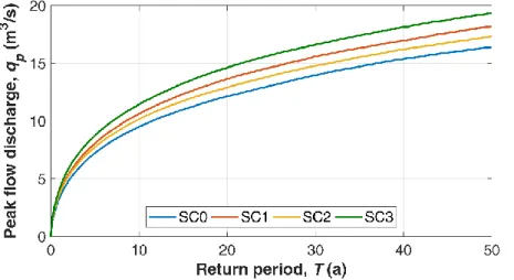
duration couples. The annual number of event was set by assuming normal distributions for the average seasonal number of rainfall events, with means and variances in accordance with estimates in Table 1. An example of the flood frequency curves, derived by using the procedure delineated in section 2, under the four climate scenarios defined in section 3, is illustrated in Figure 1, for an urban catchment characterized by an area A of 100 ha, a runoff coefficient of 0.50 and a time of concentration tc of 0.40 h.
As can be seen, all climate change scenarios determine noticeable increases in the flood
frequency, even though the total annual rainfall remains virtually unchanged. In particular, scenario 1 and scenario 2 yield quite similar outcomes demonstrating that moderate decreases in the storm durations can have effects as significant as those of rainfall depths changes. Owing to the non-linearity of the hydrological processes, scenario 3 determines peak flow discharge increases slightly less than the sum of those estimated for scenario 1 and 2. With regard to the return period of 10 a, popularly adopted in Italy for the design of urban drainage pipes, such increases amount to about 14% for scenario 1, 9% for scenario 2, and 18% for scenario 3. The ratio between the peak flow discharge and the full normal flow discharge usually spans from 0.70 to 0.80 for a drainage pipe to be suitably sized. Assuming that a drainage pipe satisfies this condition under the scenario 0, the range boundaries increase up to 0.80:0.91 under the scenarios 1, 0.75:0.87 under scenario 2, and 0.83:0.94 under scenario 3. A basically insufficient conveyance capacity is thus foreseen under climate change scenarios 1 and 2, and worsens in the case of scenario 3. Finally, the
different impacts of climate change scenarios on urban catchments featured by various combinations of hydrologic characteristics are analysed in Table 2, for T equal to 10 a.
Fig 1: Flood frequency curves derived for different scenarios (A 100 ha, 0.5, tc 0.40 h).
Tab 2: Peak flow discharges for T = 10 a, and percentage increases with respect to scenario 0 in various catchments.
Catchment characteristics Peak flow discharge qp (m
3/s) Percentage increase (%) SC0 SC1 SC2 SC3 SC1 SC2 SC3 A = 100 ha; = 0.50; tc = 0.40 h 9.51 10.80 10.40 11.20 13.6 9.4 17.8 A = 10 ha; = 0.50; tc = 0.10 h 1.81 1.99 1.97 2.24 9.9 8.8 23.8 A = 100 ha; = 0.30; tc = 0.40 h 5.75 6.37 6.18 6.85 10.8 7.5 19.1 A = 100 ha; = 0.70; tc = 0.35 h 14.66 16.27 15.52 17.16 11.0 5.9 17.1
Scenario 3 appears to mainly affect small catchments since, in this case, the percentage increase is about 24%, while for the other cases it varies in a very narrow range between 17% and 18%. Therefore, under this scenario, the climate change impact shows to be substantially independent of the catchment imperviousness. Conversely, scenarios 1 and 2 individually yield impacts more sensitive to the catchment characteristics and weaker than the one assessed for the medium impervious catchment. With regard to these medium size catchments, climate change impacts amount to about 10:14% under scenario 1, and to about 6:9% under scenario 2.
5. Conclusions
In this paper, potential impacts of climate change on small-medium size urban catchments were assessed by deriving flood frequency distributions from a bivariate distribution of rainfall volumes and storm durations. To do so, an innovative technique was developed by using copula functions, which allowed to straightforwardly implement expected climate change scenarios into the rainfall distribution. Such impacts demonstrate to be significant in the control of heavy rainfalls by means of existing drainage systems. In fact, drainage pipes are expected to fail more frequently: with respect to the return period conventionally adopted in Italy for the drainage pipe design, the estimated increases of the peak flow discharge basically exceed the pipe conveyance capacity.
References
Adams, B. J., and Papa, F. (2000), Urban stormwater management planning with analytical probabilistic models, John Wiley & Sons, New York.
Bacchi, B., Balistrocchi, M., and Grossi, G. (2008), Proposal of a semi-probabilistic approach for storage facility design, Urban Water J., 5, 3, 195-208.
Balistrocchi, M., and Bacchi, B. (2011), Modelling the statistical dependence of rainfall event variables through copula functions, Hydrol. Earth Syst. Sc., 15, 3, 1959-1977.
Balistrocchi, M., and Bacchi, B. (2017), Derivation of flood frequency curves through a bivariate rainfall distribution based on copula functions: application to an urban catchment in northern Italy’s climate, Hydrol. Res., 48, 3, 749-762.
Eagleson, S. P. (1972), Dynamic of flood frequency, Water Resour. Res., 8(9), 878-898.
IPCC (2007), Summary for policymakers, Contribution of Working Group I to the 4th Assessment Report of the Intergovernmental Panel on Climate Change, Cambridge University Press, Cambridge, UK and NY. IPCC (2014), Climate change 2014: Synthesis report, Contribution of Working Groups I, II and III to the 5th
Assessment Report of the Intergovernmental Panel on Climate Change, IPCC, Geneva, SW.
Raimondi, A., Becciu G. (2014), Probabilistic design of multi-use rainwater tanks, Procedia Engineer., 70, 1391-1400.
Salvadori, G., De Michele, C. (2006), Statistical characterization of temporal structure of storms, Adv. Water Resour. 29, 6, 827-842.
Salvadori, G., De Michele, C., Kottegoda, N. T., and Rosso, R. (2007), Extremes in nature: an approach using copulas, Springer, Dordrecht.
Wycoff, R. L., Singh, U. P. (1976), Preliminary hydrologic design of small flood detention reservoirs, Water Resour. Bull., 12, 2, 337–349.