Seismic risk computation for the fixed-base reactor building of the IRIS NPP

CONSORZIO INTERUNIVERSITARIO PER LA RICERCA TECNOLOGICA NUCLEARE

POLITECNICO DI MILANO

DIPARTIMENTO DI INGEGNERIA STRUTTURALE DIPARTIMENTO DI ENERGIA

SEISMIC RISK COMPUTATION FOR THE

FIXED-BASE REACTOR BUILDING OF THE IRIS NPP

AUTORI Giorgio Bianchi Silvia De Grandis Marco Domaneschi Davide Mantegazza Federico Perotti CIRTEN-POLIMI RL 1136/2010 Milano, Settembre 2010

Table of contents 1. Introduction

2. The FE structural model

2.1 The vessel equivalent mechanical model 2.2 The soil structure interaction simplified model

3. The assumed random variables 4. The seismic excitation

5. Design of experiments: Central Composite Design

6. Influence of the vessel damping in the structural response 7. Application of the response surface method

8. Fragility analysis

9. Application to the computation of seismic risk 10.Conclusions

References APPENDIX A

1. Introduction

This report deals with the fragility assessment of the IRIS reactor building in its original configuration, i.e. without any isolation system: the aim of the fragility computation is the comparison between the performance of the traditional and the isolated building. The latter will be investigated in a following step.

The assessment is based on the procedure described in [1], on a finite element (FE) discretization and on repeated seismic analyses performed, via the ANSYS FE code [2], with the modal superposition technique.

The most important requirement of the procedure is to reduce as much as possible the uncertainties related to the incomplete knowledge and accuracy in defining models and methods; this reduction is here sought by refining analysis procedures and using consolidated analytical and numerical tools. Secondly, the definition of the random variables is a key aspect of the analysis; the generation of the seismic excitations is the next requisite for setting up the assessment of the random vibration response of the structural system.

The computation of the exceedance probability is here performed via Monte Carlo simulation and First Order Reliability Method (FORM); to reduce the computational effort, the Response Surface (RS) method is used to express the seismic response as a function of the variation of the adopted random parameters.

The generation of the RSs is performed in terms of mean and standard deviation of the extreme value of an engineering parameter, such as the total acceleration at a given point or the AVerage floor Spectrum Acceleration (AVSA) over a frequency range.

Finally, the results of the fragility analysis are tested, also in view of a refinement of the response surfaces, within a complete risk assessment for a prototype site. The results are commented also in light of the problems associated to the hazard definition.

2. The FE structural model

The structural model has been developed at Westinghouse EC [3] along with the procedures for running the numerical analyses and extrapolating the results.

The main characteristics of the whole numerical model are here briefly summarized:

Nr. Key points . . . .. . .827 Nr. Lines . . . .1620 Nr. Areas . . . .804 Nr. Volumes . . . .4 Nr. Nodes . . . .29764 Nr. Elements. . . .36382 Nr. Element types . . . .47

Nr. Real constant sets. . . . .14017

Nr. Constraint equations. . . .10992

Figure 1 reports on the FE whole model. Figure 2 and 3 describe the x=0 and y=0 sections, respectively. It is possible to observe the reinforced concrete (RC) walls and slabs modelled by 4-node shell elements and the base of the containment, which has been treated as a rigid body.

In particular in Figure 2 are underlined the positions of the concentrated masses (indicated by “*”), which have been used for modelling, by an equivalent double-pendulum approach, the vessel, the containment and the roof of the reactor building.

Figure 2. FE model: x=0 section

Figure 3. FE model: y=0 section

2.1 The vessel equivalent mechanical model

Figure 4 reports the scheme of the structural vessel with its equivalent two-mass pendulum, called in the following equivalent mechanical model (EMM), with the main geometry characteristics.

The vessel EMM shall have the same following characteristics as the target structure, so to assure is interacts with the Auxiliary Building as the real component:

• total mass;

• position of centre of mass;

• moments of inertia about horizontal orthogonal axes through the centroid ;

• main eigenfrequencies. Additional details can be found in [3].

By assuming that the vessel undergoes a rigid body motion with horizontal translation and rotation about horizontal axes, the following equivalence relations hold:

Plan XZ x x gx

m

a

m

a

Ma

=

−

−

−

a

h

m

a

h

m

I

z

Ma

−

=

−

+

−

ϑ

&

&

a

z

a

=

+

ϑ

&

&

m

a

m

a

Ma

=

−

−

−

a

h

m

a

h

m

I

z

Ma

−

=

+

−

+

ϑ

&

&

a

h

a

=

−

ϑ

&

&

hp= 6.675 m is the level of the reactor coolant pumps (RCP) with respect to

the concrete surface supporting the vessel,

Igx=Igy= 76020000 m4 is the vessel inertia moment,

zg=0.525 m is the level of the vessel centroid,

h1=2.2 m, h2=20.9 m are the levels of the masses,

m1=1955200 kg, m2=152853 kg are the concentrated masses of the EMM,

M= m1+ m2, is the total mass of the vessel,

ϑ&& is the angular acceleration of the vessel,

a1, a2, ag, ap are the accelerations at mass 1, mass 2, vessel centroid and

RCP level.

The previous equations can be used to estimate the horizontal acceleration and rotational acceleration of the vessel, under the hypothesis that deformations are concentrated at the level of the supports. By this strategy it is possible to evaluate the horizontal acceleration (in x and y direction) at any level inside the vessel (e.g. the RCP level) starting from the FE calculated accelerations of

the two concentrated masses m1 and m2.

2.2 The soil structure interaction simplified model

Soil structure interaction (SSI) can be identified as the aspect that most highly affects the response of the auxiliary building. It represents the coupling of the structure with the soil under its foundation during a seismic excitation. A seismic response during an earthquake will depend not only on the properties of the structure itself but also on the properties of the soil around and of the excitation signal. This phenomenon, called dynamic interaction, becomes more important the higher is the

difference between the stiffness of the structure and of the soil and increases with the dimensions of the foundation due to the waves reflection and the energy absorbtion.

The soil-structure interaction is here simulated by spring and dashpot elements which connect the FE reactor building to the reference system in x, y and z directions. The properties of these elements have been defined on the basis of the “quasi-rigid foundation” hypothesis, stating that the foundation mat can be regarded as a deformable body within the structural model, but essentially behaves as rigid when the interaction with the soil is considered [4]. Under this hypothesis the spring and dashpots distributed below the foundation model match, in terms of resultants, the total stiffness and damping parameters for the six DOFs (degrees of freedom) of the rigid model [5].

Figure 4. Vessel structure with the two-masses pendulum mechanical model 3. The assumed random variables

About 23.5 m About 7 m About 11.8 m m1 m2 h2 = 2.2 m h2 = 20.9 m 17.8 m Centroid zg=0.525 m Node 30064 Node 30067 Node 30069 Node 28690 28599 28492 28781 Symbols m1 = 1955200 Kg m2 = 152853 Kg

structural main scheme pendulum mechanical model X Y X Z Y Z hp R(t), θ

Four random variables have been here selected to represent the main sources of randomness (apart from the seismic excitation) for the computation of the response of an equipment located inside the vessel.

• x1: a random variable (lognormal distribution) describing the soil shear modulus Gs, with mean value of 100MPa and c.o.v. equal to 0.3;

• x2: a random variable (lognormal distribution) describing the soil damping factor νs, with mean value of 20% and c.o.v. equal to 0.3;

• x3: a random variable (lognormal distribution) describing the concrete elastic

modulus Ec, with mean value of 21000MPa and c.o.v. equal to 0.22;

• x4: a random variable (lognormal distribution) describing the concrete damping

factor νc, with mean value of 5% and c.o.v. equal to 0.22;

The soil stiffness and damping are introduced by springs and dashpots as in Figure 3. The concrete damping is introduced in the ANSYS FE code by the material-dependent coefficient for stiffness proportional viscous damping. This is related to the damping coefficient

υ

ϖυ

β = 2 (7)

where

ϖ

4. The seismic excitation

The Response Spectra prescribed by the USNRC 1.60 (1973) [6] was adopted as seismic input. The spectral parameters were treated as deterministic, so that a single set of 20 input motions, each described by three components, has been generated and used at all experimental points. Generation was performed starting from white-noise accelerograms, modulated in the time domain, and iteratively correcting their Fourier Amplitude Spectra in order to match the USNRC 1.60 (1973) curve. An example of the accelerograms obtained is given in Figure 5.

0 10 20 30 40 time [s] -1.5 -1 -0.5 0 0.5 1 1.5 a c c e le ra ti o n [ g ] 0 1 2 3 4 5 period [s] 0 1 2 3 4 p s e u d o -a c c e le ra ti o n [ g ]

100% horizontal target spectrum 90% horizontal target spectrum generated acceleration record

Figure 5. Example of an artificial accelerogram with the target spectra from USNRC 1.60 (1973) – damping 5%.

The set of 20 input motions have been prepared by this procedure for being applied to the follow probabilistic assessment.

5. Design of experiments: Central Composite Design

For representing the reactor building response a second-order model can be used in the application of the Response Surface Method to the structural problem [1]. A full model (i.e. encompassing all quadratic terms) requires, for k random variables, the estimation of p=1+k+k(k + 1)/2 coefficients. In this situation the most suitable experimental strategy is the “Central Composite Design” (CCD); once fixed a “center point”, CCD is the combination of a classical “two-level factorial design”, in which all the combinations of two levels (high/low) of the random variables are considered, with a “star design”. In the latter 2k points are considered in which one variable takes an intermediate value and the others are at the central value. Including the central point, a total number of experiments equal to n=2k+2k+1 is reached. Reasoning in terms of non-dimensional zero-mean

random variables

η

µ

σ

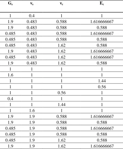
points must be placed at α =ηi =4 2k . In this study for k=4, it results p=15, n=25 andα =2. Table I summarizes the design of experiments (DoE) for the selected random variables, normalized to the mean value.

Table I. DoE with mean value normalization

Gs νs νc Ec 1 0.4 1 1 1.9 0.483 0.588 1.616666667 1.9 0.483 0.588 0.588 0.485 0.483 0.588 1.616666667 0.485 0.483 0.588 0.588 0.485 0.483 1.62 0.588 1.9 0.483 1.62 1.616666667 0.485 0.483 1.62 1.616666667 1.9 0.483 1.62 0.588 1 1 1 1 1.6 1 1 1 1 1 1 1.44 1 1 1 0.56 1 1 0.56 1 0.4 1 1 1 1 1 1.44 1 1 1.6 1 1 1.9 1.9 0.588 1.616666667 1.9 1.9 0.588 0.588 0.485 1.9 0.588 1.616666667 0.485 1.9 0.588 0.588 0.485 1.9 1.62 0.588 1.9 1.9 1.62 1.616666667

0.485 1.9 1.62 1.616666667 1.9 1.9 1.62 0.588

6. Influence of the vessel damping in the structural response

In the selection of the random variables the vessel damping has been initially taken into consideration. However, from previous analyses on an equivalent case study was shown how its variability does not contribute significantly to the structural response, in term of the selected engineering parameter (the acceleration at the RCP level), so it can be neglected [1].

As a verification, during the preliminary investigations, a structural analysis on 20 simulated

seismic accelerations has been performed. Table II reports the results in terms of mean value (a_RCP)

and standard deviation ( RCP

a

σ ) of the extreme acceleration computed at the RCP level. It is possible

to see how varying only the vessel damping and maintaining constant at their mean values the remain parameters, the statistical response does not show reasonable variations.

In light of these considerations, the vessel damping has not been considered as a structural variable provided with a significant randomness.

Table II. DoE with mean value normalization

Gs νs νv vessel damping ν_c Ec a_RCP RCP a σ 1 1 0.588 1 1 1.961706 0.1458248 1 1 1.62 1 1 1.958110 0.1467642 1 1 1 1 1 1.957478 0.1479528

Table III. Extreme absolute acceleration at the RCP level

Gs νs νc Ec RCP a RCP a σ 1 0.4 1 1 2.781052 0.181732 1.9 0.483 0.588 1.616666667 3.149629 0.191692 1.9 0.483 0.588 0.588 3.45202 0.369668 0.485 0.483 0.588 1.616666667 1.973489 0.155873 0.485 0.483 0.588 0.588 2.023667 0.138723 0.485 0.483 1.62 0.588 2.002153 0.133574 1.9 0.483 1.62 1.616666667 3.093401 0.184469 0.485 0.483 1.62 1.616666667 1.968522 0.15441 1.9 0.483 1.62 0.588 3.265414 0.361528 1 1 1 1 1.957478 0.147953 1.6 1 1 1 2.532745 0.212191 1 1 1 1.44 1.941101 0.142368 1 1 1 0.56 2.017759 0.192984 1 1 0.56 1 1.978061 0.14357 0.4 1 1 1 1.223987 0.101341

1 1 1.44 1 1.948665 0.146817 1 1.6 1 1 1.696085 0.141293 1.9 1.9 0.588 1.616666667 1.829047 0.116976 1.9 1.9 0.588 0.588 2.157065 0.180767 0.485 1.9 0.588 1.616666667 1.239875 0.11683 0.485 1.9 0.588 0.588 1.375786 0.130622 0.485 1.9 1.62 0.588 1.323353 0.126866 1.9 1.9 1.62 1.616666667 1.807637 0.117073 0.485 1.9 1.62 1.616666667 1.231432 0.118063 1.9 1.9 1.62 0.588 2.035637 0.161702

7. Application of the response surface method

Running the experiments detailed in Table I, once fixed the seismic input spectral parameters, it is possible to compute the extreme structural response at the RCP level in terms mean and standard deviation of the absolute acceleration in the horizontal plane (the acceleration vector intensity in the horizontal plane as computed with x and y components). Table III reports the 25 experiments for the central composite design and the computation of the Response Surface. The soil shear modulus modifies with more emphasis the structural response. In Appendix A are reported the absolute acceleration response time histories at the RCP and vessel supports level for three type of soil shear

modulus Gs maintaining constant the remaining ones at their mean values.

Table IV. AVSA 1-2Hz

Gs νs νc Ec RCP A σA_RCP 1 0.4 1 1 7.307136 0.530469 1.9 0.483 0.588 1.616666667 3.786385 0.120859 1.9 0.483 0.588 0.588 4.31388 0.168213 0.485 0.483 0.588 1.616666667 7.77025 0.436987 0.485 0.483 0.588 0.588 7.754443 0.487412 0.485 0.483 1.62 0.588 7.711118 0.479911 1.9 0.483 1.62 1.616666667 3.773081 0.120654 0.485 0.483 1.62 1.616666667 7.747669 0.433481 1.9 0.483 1.62 0.588 4.265076 0.159607 1 1 1 1 5.377814 0.215423 1.6 1 1 1 4.116661 0.13216 1 1 1 1.44 5.213352 0.195495 1 1 1 0.56 5.701189 0.263837 1 1 0.56 1 5.38647 0.216207 0.4 1 1 1 4.30029 0.212365 1 1 1.44 1 5.369208 0.214603 1 1.6 1 1 4.558221 0.173455 1.9 1.9 0.588 1.616666667 3.336638 0.091932 1.9 1.9 0.588 0.588 3.616884 0.116232 0.485 1.9 0.588 1.616666667 4.254613 0.20566 0.485 1.9 0.588 0.588 4.233076 0.207751 0.485 1.9 1.62 0.588 4.224263 0.206741 1.9 1.9 1.62 1.616666667 3.334459 0.091488 0.485 1.9 1.62 1.616666667 4.249733 0.205074

1.9 1.9 1.62 0.588 3.608512 0.114904

The adoption of the so called “dual response surface” approach for solving the reliability problem under stochastic input is considered. The analytical expression of the response surface has the following form for both the mean surface and the standard deviation surface:

+ + + + + + + + + + + = 0 1 1 2 2 3 3 4 4 5 1 2 6 1 3 7 1 4 8 2 3 9 2 4 10 3 4 ) (x a a x a x a x a x a x x a x x a x x a x x a x x a x x g 2 4 14 2 3 13 2 2 12 2 1 11x a x a x a x a ++ + + + (8)

The RS computation involves not only the horizontal absolute acceleration but also the averaged floor spectrum acceleration in two frequency intervals (AVSA), 1-2Hz and 2-5Hz (AVSA 1-2Hz and AVSA 2-5Hz respectively). In other words, an acceleration spectrum 3% damped is computed for all the experiments acceleration time history output in horizontal x and y direction, for each of the 20 time history samples. Only the maximum value between x and y is than considered for each one 1-2Hz and 2-5Hz intervals. Finally the mean value and the standard deviation value over 20

time histories is evaluated for each design point. Table IV and V reports the extreme values ARCP

and standard deviation RCP

A

σ in terms of AVSA at the experimental points.

Table V. AVSA 2-5Hz Gs νs νc Ec RCP A σA_RCP 1 0.4 1 1 8.481598 0.385064 1.9 0.483 0.588 1.616666667 11.93782 0.619822 1.9 0.483 0.588 0.588 11.93558 0.813467 0.485 0.483 0.588 1.616666667 3.155568 0.075547 0.485 0.483 0.588 0.588 3.170652 0.116668 0.485 0.483 1.62 0.588 3.156497 0.112947 1.9 0.483 1.62 1.616666667 11.743 0.58766 0.485 0.483 1.62 1.616666667 3.148128 0.074806 1.9 0.483 1.62 0.588 11.46948 0.707226 1 1 1 1 5.500332 0.18179 1.6 1 1 1 9.084592 0.396367 1 1 1 1.44 5.782434 0.184431 1 1 1 0.56 4.879084 0.133936 1 1 0.56 1 5.513599 0.18267 0.4 1 1 1 2.063821 0.052879 1 1 1.44 1 5.488494 0.180722 1 1.6 1 1 4.508377 0.117353 1.9 1.9 0.588 1.616666667 6.373285 0.218086 1.9 1.9 0.588 0.588 6.238751 0.205447 0.485 1.9 0.588 1.616666667 2.400567 0.051564 0.485 1.9 0.588 0.588 2.247113 0.049067 0.485 1.9 1.62 0.588 2.251127 0.048952 1.9 1.9 1.62 1.616666667 6.342643 0.214682 0.485 1.9 1.62 1.616666667 2.401576 0.051491 1.9 1.9 1.62 0.588 6.15621 0.201247

In light of these considerations the six RSs , function of four random variables, have been processed by an ordinary least squares method and the following a0-14 parameters result.

RCP absolute acceleration (MEAN) a0=1.986767707; a1=2.261109248; a2=-2.059244968; a3=1.19E-02; a4=-4.38E-02; a5=-0.422690008; a6=-0.297249737; a7=-5.74E-02; a8=-0.130951806; a9=0.734595069; a10=1.00E-02; a11=-4.11E-02; a12=-3.80E-02; a13=6.62E-02; a14=8.07E-03;

RCP absolute acceleration (STANDARD DEVIATION) a0=0.153058732; a1=0.219873571; a2=-5.16E-02; a3=5.69E-02; a4=-0.187734841; a5=-1.61E-04; a6=-5.62E-02; a7=-5.05E-03; a8=-8.30E-02; a9=1.34E-02; a10=-6.40E-04; a11=3.11E-02; a12=-2.82E-02; a13=6.48E-03; a14=8.56E-02; AVSA 1-2Hz (MEAN) a0=12.08381275; a1=4.360644212; a2=-8.066750513; a3=-2.377333182; a4=-3.808669312; a5=-3.044135739; a6=1.445149064; a7=-2.33E-02; a8=-0.302780408; a9=2.033693858; a10=2.71E-03; a11=7.28E-02;

a12=1.084985892;

a13=39.06E-03;

a14=1.765669193;

AVSA 1-2Hz (STANDARD DEVIATION) a0=0.839138718; a1=0.203965487; a2=-1.120557626; a3=0.172724883; a4=-9.28E-02; a5=-0.198212087; a6=0.107294605; a7=9.87E-05; a8=-5.12E-03; a9=0.358419583; a10=4.45E-03; a11=2.51E-02; a12=-8.52E-02; a13=5.17E-03; a14=1.41E-02; AVSA 2-5Hz (MEAN) a0=-2.467263779; a1=10.03382239; a2=-5.666644261; a3=2.697221384; a4=5.998668132; a5=-1.113923658; a6=-2.323411686; a7=-0.139826832; a8=2.56E-02; a9=2.495470841; a10=0.122579963; a11=6.95E-02; a12=-1.299132153; a13=7.12E-02; a14=-2.745527477;

AVSA 2-5Hz (STANDARD DEVIATION) a0=-5.07E-02; a1=0.385736192; a2=-0.443144087; a3=8.77E-02; a4=0.40422987; a5=8.51E-02; a6=-0.213270791; a7=-2.47E-02; a8=-3.89E-02; a9=0.172529498; a10=2.31E-02;

a11=7.08E-02;

a12=-5.49E-02;

a13=1.61E-02;

a14=-0.226138886;

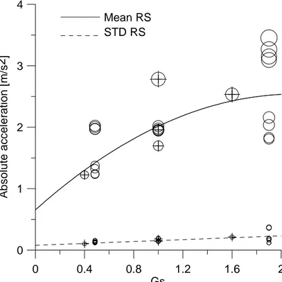
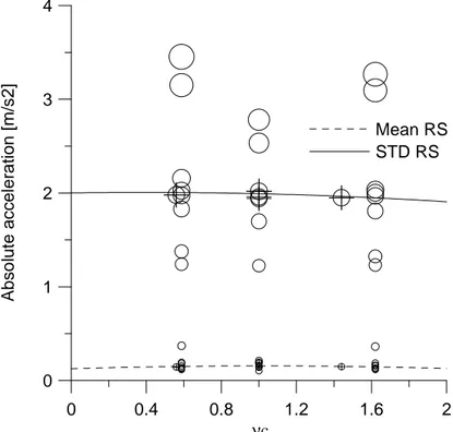
Figures 6-9 depict the main sections of the RSs in terms of both mean and standard deviation for the absolute acceleration at the RCP level. They are computed maintaining constant respectively x2-x3

-x4=1, x1-x3-x4=1, x1-x2-x4=1, x1-x2-x3=1. It is worth noting that the acceleration variability is more evident with the variation of the soil characteristics. The concrete properties variability seems to stress less the maximum acceleration response at the RCP level. This behavior emphasizes how the site characteristics can modify the structural response. The “+” symbols and “O” symbols in the figures reflect the experimental points on the same section and the remaining experimental points respectively.

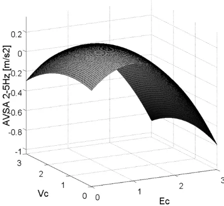
Figure 10-13 reports the RSs processed maintaining constant respectively x3-x4=1, x1-x2=1. Figure 14-21 depict the RSs for AVSA 1-2Hz and 2-5Hz.

0 0.4 0.8 1.2 1.6 2 Gs 0 1 2 3 4 A b s o lu te a c c e le ra ti o n [ m /s 2] Mean RS STD RS

0 0.4 0.8 1.2 1.6 2 νs 0 1 2 3 4 A b s o lu te a c c e le ra ti o n [ m /s 2] Mean RS STD RS

Figure 7. Absolute acceleration RS: section x1=x3=x4=1

0 0.4 0.8 1.2 1.6 2 νc 0 1 2 3 4 A b s o lu te a c c e le ra ti o n [ m /s 2 ] Mean RS STD RS

0 0.4 0.8 1.2 1.6 2 Ec 0 1 2 3 4 A b s o lu te a c c e le ra ti o n [ m /s 2 ] Mean RS STD RS

Figure 9. Absolute acceleration RS: section x1=x2=x3=1

Figure 11. Absolute acceleration RS: surface “STD” x3=x4=1

Figure 13. Absolute acceleration RS: surface “STD” x1=x2=1

Figure 15. AVSA 1-2Hz RS: surface “STD” x3=x4=1

Figure 17. AVSA 1-2Hz RS: surface “STD” x1=x2=1

Figure 19. AVSA 2-5Hz RS: surface “STD” x3=x4=1

Figure 21. AVSA 2-5Hz RS: surface “STD” x1=x2=1

8. Fragility analysis

The fragility functions have been computed by the “hit or miss” Monte Carlo Method (MCM) and a First Order Reliability Method (FORM) [1, 7-9].

The RS supports the computational procedures. In particular the application of the MCM consists in a sequential generation of samples of lognormal variables (x1 x2 x3 x4).

Taking into account the probabilistic parameters of a lognormally distributed random variable, one can evaluate the parameters of the variable’s natural logarithm (by definition, the variable’s logarithm is normally distributed) as

      + + = ₂ ) X ( ) X ( 1 ln 5 . 0 ) X ( ln( a

Μ

Σ

Μ

Μ

Σ

σ

where a and

σ

VI reports the main normalized random variables statistic parameters where X is a random

variable with a lognormal distribution, then Y = ln(X) has a normal distribution.

For each sample extracted by the lognormal distributions it is possible to evaluate, by the mean and standard deviation response surfaces, the probability density function of the structural response in terms of extreme values of absolute acceleration, AVSA 1-2Hz and AVSA 2-5Hz. The mean and standard deviation computed via the RSs, in fact, are subsequently used for extracting the acceleration demand from the Gumbel distribution for the extreme value; the

extracted value is compared to the critical threshold. By this procedure the exceedance probability is evaluated and the MCM fragility curve is completed.

Table VI. Normalized random variables statistic parameters

Lognormal Normal Gs Μ(X)=1 Σ(X)=0.3 ā _=-0.04309 σ =0.29356 σ 2_=0.086178 ν_s Μ(X)=1 Σ(X)=0.3 ā _=-0.04309 σ _=0.29356 σ 2_=0.086178 ν_c Μ(X)=1 Σ(X)=0.22 ā _=-0.02363 σ _=0.217406 σ 2=0.047265 Ec Μ(X)=1 Σ(X)=0.22 ā =-0.02363 σ _=0.217406 Σ 2_=0.047265

Figure 22 depicts three fragility functions processed by MCM. The fragility is represented as the

probability of exceeding the amplification a_RCP/a_g or AVSA_RCP/a_g.

The AVSA functions emphasize the amplification of the response of a component; it shows how the probability of failure can be incremented when the peak acceleration of a component, averaged over a fixed range of natural frequencies, is considered. In the example here shown, the AVSA functions describe the fragility of a component located at RCP level when its main natural frequency is into the 1-2Hz or 2-5Hz frequency ranges.

1 2 3 4 5 6 7 8 9 10 11 12 Amplification (a/ag) 0 0.2 0.4 0.6 0.8 1 P f Absolute acceleration AVSA 1-2 Hz AVSA 2-5 Hz

1 2 3 4 Amplification (a/ag) 0 0.2 0.4 0.6 0.8 1 P f Absolute acceleration MCM Absolute acceleration FORM

Figure 23. RCP absolute acceleration. Fragility curves: MCM and FORM

1 2 3 4 5 6 7 8 9 10 Amplification (a/ag) 0 0.2 0.4 0.6 0.8 1 P f AVSA 1-2 Hz MCM AVSA 1-2 Hz FORM

1 2 3 4 5 6 7 8 9 10 11 12 13 14 15 Amplification (a/ag) 0 0.2 0.4 0.6 0.8 1 P f AVSA 2-5 Hz MCM AVSA 2-5 Hz FORM

Figure 25. AVSA 2-5 Hz. Fragility curves: MCM and FORM

The application of FORM allows to compute the fragility functions in a alternative way. The probability of failure is computed, for each amplification, as the distance (from the origin) of the tangent plane to the limit state function at the design point.

Once the design point is found, the evaluation of Pf is rapidly performed. The comparison between

the three curves in Figure 22 is reported by Figures 23-25, respectively for the absolute acceleration, the AVSA 1-2Hz and 2-5Hz.

9. Application to the computation of seismic risk

The remaining of this report is devoted to the evaluation of the seismic risk by integrating the hazard and fragility evaluations. In particular it is considered the absolute acceleration fragility function as processed by FORM (Figure 23).

Figure 26. Seismic hazard

Figure 27. PDF

The problem of establishing the hazard curve is complex due to the fact the statistical parameters over a certain limit, in terms of return period, lacks of observable data. Therefore, some assumptions have been introduced. The hazard is related to a site described by return period vs ground acceleration in Figure 26.

In the estimation of the seismic risk two hypotheses has been introduced:

1) the PDF (probability density function, Figure 27) for the hazard is extended and truncated to

16m/s2 (Figure 28);

Figure 28. Detail: PDF extended and truncated to 16m/s2

Figure 29. Detail: PDF extended to 20m/s2

Following these two assumptions, the probability of failure has been computed for several failure

accelerations (af), related to a component at the RCP level. In particular af = 5, 10, 15, 20, 25, 30,

35, 40 m/s2 have been considered. The results are reported for extended and truncated PDF in

Figures 30-37; for extended PDF, with no truncation, in Figures 38-45. For the highest failure accelerations levels the failure probabilities obtained from the non-truncated PDF are only rough approximations, due to the fact the fragility times hazard function is non-zero in a wider acceleration domain.

Table VII summarizes the probabilities of failure for the considered component acceleration thresholds.

Figure 30. 16m/s2 extended and truncated PDF af = 5m/s2 . Fragility times hazard vs pga and failure probability vs pga (dashed).

Figure 31. 16m/s2 extended and truncated PDF, af = 10m/s2 . Fragility times hazard vs pga and failure probability vs pga (dashed).

Figure 32. 16m/s2 extended and truncated PDF, af = 15m/s2 . Fragility times hazard vs pga and failure probability vs pga (dashed).

Figure 33. 16m/s2 extended and truncated PDF, af = 20m/s2 . Fragility times hazard vs pga and failure probability vs pga (dashed).

Figure 34. 16m/s2 extended and truncated PDF, af = 25m/s2 . Fragility times hazard vs pga and failure probability vs pga (dashed).

Figure 35. 16m/s2 extended and truncated PDF, af = 30m/s2 . Fragility times hazard vs pga and failure probability vs pga (dashed).

Figure 36. 16m/s2 extended and truncated PDF, af = 35m/s2 . Fragility times hazard vs pga and failure probability vs pga (dashed).

Figure 37. 16m/s2 extended and truncated PDF, af = 40m/s2 . Fragility times hazard vs pga and failure probability vs pga (dashed).

Figure 38. 20m/s2 extended PDF, af = 5m/s2 .

Fragility times hazard vs pga and failure probability vs pga (dashed).

Figure 39. 20m/s2 extended PDF, af = 10m/s2 .

Figure 40. 20m/s2 extended PDF, af = 15m/s2 . Fragility times hazard vs pga and Pf vs pga (dashed).

Figure 41. 20m/s2 extended PDF, af = 20m/s2 .

Figure 42. 20m/s2 extended PDF, af = 25m/s2 .

Fragility times hazard vs pga and failure probability vs pga (dashed).

Figure 43. 20m/s2 extended PDF, af = 30m/s2 .

Figure 44. 20m/s2 extended PDF, af = 35m/s2 .

Fragility times hazard vs pga and failure probability vs pga (dashed).

Figure 45. 20m/s2 extended PDF, af = 40m/s2 .

Table VII. Failure probabilities af [m/s2] Pf (16m/s2 extended and truncated PDF) Pf (20m/s2 extended PDF) 5 2.22E-04 2.23E-04 10 2.84E-05 2.85E-05 15 7.49E-06 7.65E-06 20 2.50E-06 2.66E-06 25 8.51E-07 9.94E-07 30 2.64E-07 3.72E-07 35 6.97E-08 1.36E-07 40 1.52E-08 4.74E-08 10.Conclusions

This study reports about the seismic risk computation of the not-isolated IRIS Reactor Building. A previously developed FE model of the Auxiliary Building is adopted and several random parameters are selected. The fragility analysis of the IRIS Reactor Building is then performed by consolidated analytical and numerical tools. The attention is focused at a point inside the vessel at the RCP level. The seismic risk is finally computed by considering an hazard curve related to a medium seismicity site with two different extended PDFs (truncated and not truncated). The resulting seismic risks, for both the hazard characteristics, points out that the new circular plant of the not-isolated IRIS has a lower seismic response than the previous version with rectangular plan (see also [1]); this is probably due to the large embedment, which has been explicitly modelled in the last version of the IRIS Reactor Building.

References

1. De Grandis S., Domaneschi M., Perotti F., “A numerical procedure for computing the fragility of NPP components under random seismic excitation”, Nuclear Engineering and Design, Volume 239, Issue 11, November 2009, Pages 2491-2499, ISSN 0029-5493, DOI: 10.1016/j.nucengdes.2009.06.027. 2. Ansys Academic Research, v. 11.0. Ansys Inc., Canonsburg, PA, United States.

3. IRIS NNP Seismic Anlysis, Calculation Note, 2008 Westinghouse Electric Company LLC.

4. Bianchi G., Mantegazza D.C., Perotti F., ‘Dynamic Modelling for the Assessment Of Seismic Fragility of NPP Components’, Proc. of Intl Conf on Structural Mechanics in Reactor Technology (SMIRT 19), paper id K14/3, Toronto 12-17 Aug, 2007.

5. Sieffert J.G., Cevaer F., “Handbook of Impedance Function”, Ouest Editions, Presses Academiques, 1992. ISBN 2-908261-32-4.

6. USNRC 1.60 - Design Response Spectra For Seismic Design Of Nuclear Power Plant, Regulatory Guide, U.S. Atomic Energy Commission, December 1973.

7. Perotti F., Domaneschi M., De Grandis S., “A procedure for the computation of seismic fragility of equipment components in NPPs”, 20th International Conference on Structural Mechanics in Reactor Technology (SMIRT20), August 9-14, 2009, Espoo Finland.

8. Rubinstein R.Y., “Simulation ad the Montecarlo Method”, Wiley 1981. ISBN 0-471-08917-6. 9. Kennedy R.P., “Overview of Methods for Seismic PRA and Margin Analysis Including Recent

Innovations”, Proceedings of the OECD-NEA Workshop on Seismic Risk, Tokyo Japan, 10-12 August 1999.

-2.5 -2.0 -1.5 -1.0 -0.5 0.0 0.5 1.0 1.5 2.0 2.5 0 5 10 15 20 25 30 Time [s] A c ce le ra ti o n [ g ] X pump acc. X support acc.

Figure A1. X direction absolute acceleration.

Soil shear modulus Gs = 1 (νs=νc=Ec=1, Input Time History 1).

-2.5 -2.0 -1.5 -1.0 -0.5 0.0 0.5 1.0 1.5 2.0 2.5 0 5 10 15 20 25 30 Time [s] A c ce le ra ti o n [ g ] X pump acc. X support acc.

Figure A2. X direction absolute acceleration.

-2.5 -2.0 -1.5 -1.0 -0.5 0.0 0.5 1.0 1.5 2.0 2.5 0 5 10 15 20 25 30 Time [s] A c ce le ra ti o n [ g ] X pump acc. X support acc.

Figure A3. X direction absolute acceleration.

Soil shear modulus Gs = 0.485 (νs=νc=Ec=1, Input Time History 1).

-2.5 -2.0 -1.5 -1.0 -0.5 0.0 0.5 1.0 1.5 2.0 2.5 0 5 10 15 20 25 30 Time [s] A c ce le ra ti o n [ g ] Y pump acc. Y support acc.

Figure A4. Y direction absolute acceleration.

-2.5 -2.0 -1.5 -1.0 -0.5 0.0 0.5 1.0 1.5 2.0 2.5 0 5 10 15 20 25 30 Time [s] A c ce le ra ti o n [ g ] Y pump acc. Y support acc.

Figure A5. Y direction absolute acceleration.

Soil shear modulus Gs = 1.9 (νs=νc=Ec=1, Input Time History 1).

-2.5 -2.0 -1.5 -1.0 -0.5 0.0 0.5 1.0 1.5 2.0 2.5 0 5 10 15 20 25 30 Time [s] A c ce le ra ti o n [ g ] Y pump acc. Y support acc.

Figure A6. Y direction absolute acceleration.