EVALUATION OF ARTIFICIAL NEURAL
NETWORKS PERFORMANCES ON SPECTRAL
CLASSIFICATION TASKS
S. DI FRISCHIA, F. ANGELINIFusion and Technology for Nuclear Safety and Security Department Frascati Research Centre, Rome, Italy
RT/2019/6/ENEA
ITALIAN NATIONAL AGENCY FOR NEW TECHNOLOGIES, ENERGY AND SUSTAINABLE ECONOMIC DEVELOPMENT
S. DI FRISCHIA, F. ANGELINI
Fusion and Technology for Nuclear Safety and Security Department Frascati Research Centre, Rome, Italy
EVALUATION OF ARTIFICIAL NEURAL
NETWORKS PERFORMANCES ON SPECTRAL
CLASSIFICATION TASKS
RT/2019/6/ENEA
ITALIAN NATIONAL AGENCY FOR NEW TECHNOLOGIES, ENERGY AND SUSTAINABLE ECONOMIC DEVELOPMENT
I rapporti tecnici sono scaricabili in formato pdf dal sito web ENEA alla pagina www.enea.it I contenuti tecnico-scientifici dei rapporti tecnici dell’ENEA rispecchiano
l’opinione degli autori e non necessariamente quella dell’Agenzia
The technical and scientific contents of these reports express the opinion of the authors but not necessarily the opinion of ENEA.
EVALUATION OF ARTIFICIAL NEURAL NETWORKS PERFORMANCES ON SPECTRAL CLASSIFICATION TASKS
S. Di Frischia, F. Angelini
Abstract
This report is a preliminary study about the evaluation of the Artificial Neural Network (ANN) perfor-mances in a spectral classification scenario. Several different ANN architectures has been tested in order to solve signal identification tasks, starting from a simple input set and refining the task step to step. Since the aim is to define in the future a robust method to classify Raman spectra in non-labora-tory conditions, the input set has been built as a Raman-like spectra set, with noisy signals containing narrow Gaussian peaks..
The behavior of the neural networks has been evaluated varying the main input properties and analy-zing the standard ANN key performance indicators. All the tests in this paper have been developed and generated with MATLAB®.
After a description of the artificial neural networks and their features, the report analyzes the task identification, the noise definition and some concepts in the statistic theory field. Then, a series of tests with their performance plots are illustrated, both with artificial spectra and real laboratory spectra generated with a mercury-vapor lamp. In the end, the report produces a list of conclusions with some further analysis and task refinements to do.
Key words: algorithms, artificial intelligence, neural networks, raman, spectroscopy, spectral classi-fication, signal processing, pattern recognition.
Riassunto
Questo documento presenta uno studio preliminare riguardo la valutazione delle performance di una rete neurale artificiale (ANN) in uno scenario di classificazione spettrale. Differenti architetture di reti neurali sono state testate al fine di risolvere problemi di identificazione spettrale, iniziando da un sem-plice insieme di input, per poi raffinare il problema un passo alla volta. Dato che l’obiettivo in futuro è quello di definire un sistema robusto ed efficiente per la classificazione di spettri Raman in condizioni non di laboratorio, l’insieme di spettri di input è stato costruito sul modello di spettri Raman, con se-gnali rumorosi contenenti picchi gaussiani stretti.
Il comportamento delle reti neurali è stato valutato variando le principali proprietà di input, e analiz-zando gli indicatori chiave di performance delle reti neurali. Tutti i test contenuti in questo documento sono stati sviluppati e generati con il software MATLAB®.
Dopo una descrizione generale delle reti neurali e delle loro proprietà, il documento analizza l’identi-ficazione del problema, la definizione di rumore e alcuni concetti nel campo dell’inferenza statistica. Quindi, vengono illustrati una serie di test con i relativi grafici di performance, in cui sono stati usati sia spettri artificiali che spettri reali generati in laboratorio con una lampada a vapori di mercurio. Alla fine del documento sono state prodotte una serie di conclusioni, con ulteriori analisi e raffinamenti del problema da eseguire in futuro.
Parole chiave: algoritmi, intelligenza artificiale, reti neurali, raman, spettroscopia, classificazione spettrale, analisi dei segnali, pattern recognition.
1 ARTIFICIAL NEURAL NETWORK DESCRIPTION 1.1 Neural Networks with MATLAB
2 TASK IDENTIFICATION AND REDUCTION 2.1 Input Data
2.2 Target Vector 3 SIGNAL / NOISE RATIO 4 NOISE POWER SPECTRUM
5 FALSE POSITIVES AND FALSE NEGATIVES 6 PATTERN RECOGNITION TASK
6.1 Plot Explanation
7 ARTIFICIAL NEURAL NETWORK TEST
7.1 TEST 1: Processing Time vs. Input Vector Dimension 7.2 TEST 2: Signal To Noise Ratio vs Accuracy
7.3 TEST 3: Layer Size vs Accuracy
7.4 TEST 4 - Refine the task: Peak Position vs Accuracy
7.5 TEST 5 - Refine the task: Discrimination between two Gaussian signals 8 LABORATORY TEST 9 CONCLUSIONS 10 REFERENCES 7 10 11 12 15 17 19 22 22 24 29 29 35 46 54 59 67 72 74
INDEX
7
1 ARTIFICIAL NEURAL NETWORK DESCRIPTION
An Artificial Neural Network (ANN) is a computing system made up of a number of highly interconnected elements which process information by their dynamic response to external inputs. It is inspired by the biological neural network. An ANN learn by examples, so every ANN is configured for a specific application, such as pattern recognition, data classification, and so on.
The ANNs are composed of multiple nodes (neurons). The nodes are connected by links and they interact with each other. The nodes can take input data and perform simple operations on the data. The result of these operations is passed to other neurons. The output at each node is called its activation or node value. The advantages of using ANNs include:
• Adaptive learning • Self-organization • Real-Time Operation • Fault Tolerance
An artificial neuron is a device with many inputs and one output. The neuron has two mode of operation: the training mode and the using mode. In the training mode, the neuron can be trained to fire (or not), for particular input patterns. In the using mode, when a taught input pattern is detected at the input, its associated output becomes the current output. If the input pattern does not belong in the taught list of input patterns, the firing rule is used to determine whether to fire or not.
A more sophisticated neuron (Figure 1) accepts a set of weighted inputs: the effect that each input has at decision making is dependent on the weight of the particular input. These weighted inputs are then added together and if they exceed a pre-set threshold value, the neuron fires. In any other case, the neuron does not fire.
In mathematical terms, the neuron fires if and only if:
8
Figure 1 - Artificial Neuron Representation
There are two main architectures in ANNs : Feed-forward networks and Feedback networks.
Feed-Forward ANNs allow signals to travel one way only: from input to output.
Feedback ANNS can have signals travelling in both directions by introducing loops in the network.
Feedback networks are dynamic: their state is changing continuously until they reach an equilibrium point. The most common type of ANN consists in three groups, or layers, of units: a layer of input units is connected to a layer of hidden units, which is connected to a layer of output units (Figure 2).
9 Every neural network possess knowledge which is contained in the values of the connections weights. We can represent this knowledge as a weight matrix W of the network. The process of learning is basically the determination of the weights. All the learning methods used for adaptive ANNs (able to change their weights) can be classified in two major categories:
• Supervised learning: where each output unit is told what its desired response to input signals ought to be.
• Unsupervised learning: where there is no external teacher and is based upon only local information. It self-organises data presented to the network and detects their emergent collective properties. We say that a neural network learns off-line if the learning phase and the operation phase are distinct. A neural network learns on-line if it learns and operates at the same time.
The behaviour of an ANN depends on both the weights and the input-output function (transfer function) that is specified for the units. This function typically falls into one of three categories:
• Linear (or ramp) • Threshold • Sigmoid
In order to train a neural network to perform some task, we must adjust the weights of each unit in such a way that the error between the desired output and the actual output is reduced. This process requires that the neural network compute the error derivative of the weights (EW). In other words, it must calculate how the error changes as each weight is increased or decreased slightly. The back-propagation algorithm is the most widely used method for determining the EW.
The motivation for backpropagation is to train a multi-layered neural network such that it can learn the appropriate internal representations to allow it to learn any arbitrary mapping of input to output.
Here is a simple explanation of the back-propagation algorithm:
A unit in the output layer determines its activity by following a two-step procedure: • First, it computes the total weighted input xj
• Next, the unit calculates the activity yj using some function of the total weighted input. Typically we
use the sigmoid function
Once the activities of all output units have been determined, the network computes the error E. The back-propagation algorithm consists of four steps:
1. Compute how fast the error changes as the activity of an output unit is changed. This error derivative (EA) is the difference between the actual and the desired activity.
2. Compute how fast the error changes as the total input received by an output unit is changed. This quantity (EI) is the answer from step 1 multiplied by the rate at which the output of a unit changes as its total input is changed.
10
3. Compute how fast the error changes as a weight on the connection into an output unit is changed. This quantity (EW) is the answer from step 2 multiplied by the activity level of the unit from which the connection emanates.
4. Compute how fast the error changes as the activity of a unit in the previous layer is changed. This crucial step allows back-propagation to be applied to multilayer networks. When the activity of a unit in the previous layer changes, it affects the activities of all the output units to which it is connected. So to compute the overall effect on the error, we add together all these separate effects on output units. But each effect is simple to calculate. It is the answer in step 2 multiplied by the weight on the connection to that output unit.
By using steps 2 and 4, we can convert the EAs of one layer of units into EAs for the previous layer. This procedure can be repeated to get the EAs for as many previous layers as desired. Once we know the EA of a unit, we can use steps 2 and 3 to compute the EWs on its incoming connections.
1.1 Neural Networks with MATLAB
We decided to use MATLAB for our tests with the ANNs mainly because of its powerful Neural Network Toolbox. MATLAB has four Neural Networks toolbox for the following tasks:
• Data Clustering (nctool) • Function Fitting (nftool) • Pattern Recognition (nprtool) • Time-Series Analysis (ntstool)
The end-user can decide whether to use the ANN functionalities through the toolboxes or through the command-line operations. Anyway, a combination of the two techniques suits better our problem.
We will proceed in the design of the neural network to solve our task with the following steps: • Identify the task
• Collect data • Create the network • Configure the network • Initialize the weights • Train the network • Validate the network • Use the network
11
2 TASK IDENTIFICATION AND REDUCTION
Our task falls into the field of Spectral Identification/Recognition. Each type of spectroscopy produces spectra of different characteristics from the point of view of the signal analysis and provides a different physical information. The chemical species recognition from any kind of spectrum is a problem that has numerous fields of application: Medicine, Biology, Industrial Processes, Safety and Security. However, at present day, there are no universally accepted algorithms for automatic spectral recognition. Under "non-laboratory" conditions the problem is complex due to the overlap of interfering substances and the contribution of background noise.
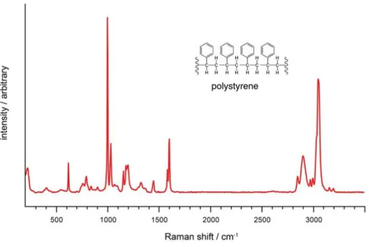
Initially we will focus on RAMAN spectroscopy, due to the characteristics of its spectra that we will discuss below. RAMAN spectroscopy is an analysis technique based on the Raman effect, an inelastic scattering of photons produced by the excited sample. In fact, a part of the incident light beam towards a sample is scattered elastically (same frequency, Rayleigh effect), while a minor part is scattered with a different frequency from the original one (Raman effect). The energetic difference between the incident photons and the inelastically scattered photons corresponds to the vibrational energy levels of the molecule: the analysis of the displacement of the spectral lines due to the Raman effect can therefore provide information on the chemical composition, the molecular structure and the intermolecular interactions of the sample.
Figure 3 - RAMAN spectrum
The Figure 3 - RAMAN spectrum contains a typical RAMAN spectrum acquired in “laboratory” conditions. Its main features are the narrow peaks, whose relative positions and amplitudes are characteristic of the molecule. Our task of Spectral Recognition presents itself apparently as a simple problem: performing a matching between the measured spectrum and a known reference spectrum. However, the issues of this approach are numerous:
12
• The contribution of noise in the measured spectrum that makes inefficient a simple vector similarity (for example the Euclidean distance)
• The alignment problem of the main peak, that can shift around a small interval on the x-axis • The compresence of various substances (and hence of various peaks) on the sample
• The contribution of fluorescence in the measured spectrum
In the past years different approaches based on the Artificial Neural Networks have been proposed to solve this challenging task. We will proceed step by step in the design and implementation of an ANN that can suits our problem. Beginning with a simple classification of random spectra, we will refine subsequently the network with more complex structures and targets.
Initially, our aim is to use an Artificial Neural Network in order to classify a set of random noisy spectra respect to a target vector. Half of these spectra set are Gaussian signals with noise, the other half are pure noisy signals. The ANN that we want to create should classify these spectra as a Gaussian or not.
2.1 Input Data
To create a certain number of input random vectors for the task: • Define the dimension of each vector (Lx)
• Define the total number of vectors (N) N=10000;
Lx=100;
• Create a Gaussian function G = gaussmf(1:Lx,[Lx/20 Lx/2]);
13 • Create a random set (dimension N) of noisy signals
R=randn(Lx,N);
• Sum the noisy signals with the Gaussian
G = repmat(G',1,N)+R;
14
15
2.2 Target Vector
Once that we have created the set with the Gaussian and the random signals, we must define the Target set of our ANN. The Target Vector T is the desired output for the given input X. The ANN will be trained with the known input X and the target T in the first phase. Then, in the test phase, the ANN will produce the
output Y as a result of the processing of input X. The error is computed as E = T-Y, and of course the
ultimate goal is to minimize this error function.
Since that we want to classify the input vectors as Gaussian or not, our target vector contains a value of 1 in the same position of a Gaussian input vector, and a value of 0 in case of a random noisy signals.
For example:
Input vector = [G , R, G, G, R] Target vector = [1 , 0 , 1 , 1 , 0]
As mentioned above, we created a N=10000 of input signals, and for simplicity we put the Gaussian signals in the first half and the random signals in the second half. So, in this case our vector target is an array of length N, where the values are 1 in the interval [0:N/2] and 0 in the interval [N/2:0]
T=zeros(1,N); %target vector
16
3 SIGNAL / NOISE RATIO
The Signal/Noise Ratio (SNR or S/N) is a measure that compares the level of a desired signal to the level of background noise in any system that acquires, processes or transmits information.
SNR is defined as the ratio of signal power to the noise power, and expresses how powerful is the signal compared to the noise; these two measures are often expressed in decibel (db) or Watt (W).
18
4 NOISE POWER SPECTRUM
We already stated that a random MATLAB function will be used to generate random vectors that will simulate the noise in the tests below (R=randn(Lx,N)). But which kind of noise is this?
If we plot an histogram of the command above, we obtain a (almost nearly) Gaussian distribution, as depicted in the image below on a set of N=10000 values.
This means that the generated noise is a white noise. In other words, it is a random signal that has equal intensity at different frequency intervals. It can also be defined as a series of uncorrelated random variables that evolves over time with a zero mean. Since that its instant values are not correlated, the white noise in a spectral classification task can be sensibly decreased with a mean of a certain number of vectors acquired at different time. Hence, using the mean, at any frequency the signal variations are balanced.
In the image below it is represented a noise power spectrum of the MATLAB generated random vectors. It is clear that the power is reasonably constant at any period (so at any frequency).
19 The question is that the optical devices used in practical experiments show a different kind of noise: the Pink
Noise (often referred as flicker noise). In the pink noise the power spectral density is inversely proportional
to the frequency of the signal.
In this case, the instant noise value is not independent from the previous instant value, since some frequencies (the low ones) are more probable and hence, the rapid fluctuations (typical of the white noise) are disadvantaged. So, in a spectral classification task, the mean of the vectors doesn’t apparently reduce the noise beyond a certain threshold.
In the image below it is represented a noise power spectrum of some laboratory acquired spectra. The pink noise is clearly visible with the power increasing with the value of the period (at low frequencies).
For now, in the tasks presented in this paper, we keep on use the white noise simulation. But in the future tests it will be important to deal with the different kind of noises generated in real experiments conditions.
20
5 FALSE POSITIVES AND FALSE NEGATIVES
In statistic test theory, false positives and false negatives are the two types of error distinguished in the result of a test. They are more correctly defined as Type I Error (FP) and Type II Error (FN).
A type I error occurs when the null hypothesis (H0) is true, but is rejected. It is asserting something that is absent, a false hit. A type I error may be likened to a so-called false positive (a result that indicates that a given condition is present when it is actually not present).
A type II error occurs when the null hypothesis is false, but erroneously fails to be rejected. It is failing to assert what is present, a miss. A type II error may be compared with a so-called false negative (where an actual 'hit' was disregarded by the test and seen as a 'miss') in a test checking for a single condition with a definitive result of true or false. A Type II error is committed when we fail to believe a true alternative hypothesis.
In our ANN classification examples, one of the most important features to validate the neural network is to reach the minimal numbers of false positives. In this case, the false positives are the Random Noisy
Signals classified as Gaussian Signals. This type error means that the system has wrongly classified an
unwanted signal in our set of target signals.
Otherwise, the false negatives are Gaussian Signals that are not recognized, but are “missed”. This kind of error is also an important indicator of the quality of the ANN, but normally is less frequent than the False Positive Error.
6 PATTERN RECOGNITION TASK
We will use the Matlab Neural Network Tool to validate and test our ANN in different configurations. In detail, the Pattern Recognition Tool (nprtool) will be used with the input and target set defined in the
21 previous paragraphs. This kind of tool is the one that suits more our problem definition, since we want to build a neural network that classify inputs into a set of target categories.
Before deploying the neural network, we must define three primary features in the process of ANN creation: • Number of layers and sizes of the hidden layer
• Training function
• Perform function (objective function to minimize)
These features are set initially with default values, because we want to focus on other properties of the network that will be changed to investigate the results achieved by the ANN. The default values are:
• 1 Hidden Layer with size (neuron number) of 10. The transfer function to the Output Layer is set as a sigmoid.
• The Scaled conjugate gradient backpropagation (Moller, 1990) as the training function.
• The Cross-Entropy function as the perform function. This function returns a result that heavily penalizes outputs that are extremely inaccurate (y near 1-t), with very little penalty for fairly correct classifications (y near t). Minimizing cross-entropy leads to good classifiers.
In addition, we will divide randomly our set of input vector (N) in three kind of samples with this percentages:
• 70% Training. These samples are presented to the network during training, and the network is adjusted according to its error.
• 15% Validation. These samples are used to measure network generalization, and to halt training when generalization stops improving.
• 15% Testing. These samples have no effect on training and so provide an independent measure of network performance during and after training.
6.1 Plot Explanation
Here is an explanation of the plot that will be used later to test the accuracy and the performance of the different instances of our pattern recognition ANN.
22
This window is presented after a graphic representation of the structure of ANN and a list of the algorithms used. The parameters are:
o Epoch. It can be thought as a completed iteration of the training procedure of the ANN. When all the input vectors have been used by the training algorithm, 1 epoch is passed, and the ANN begin a new iteration (epoch).
o Time. It’s the entire ANN processing time. It includes training, validation and test.
o Performance. It’s the value of our performance function. For a good ANN it must be closer to 0 as possible
o Gradient. It’s the gradient value of our training function. The back-propagation uses a descent gradient approach to minimize the error function. At each epoch the weight vector is modified towards the direction that produces the sharpest gradient descent
o Validation Checks. For default is set at a value of 6. It means that if after 6 epochs the validation dataset (non-training) don’t decrease the performance function, the training is stopped. In other words, the last 6 epochs are the ones that apparently don’t improve the accuracy of the network
23 In this plot we have the epochs on the x-axis and the value of our error function to minimize on the y-axis. It shows the trend of training, validation and test performance of the ANN. Generally, the error reduces after more epochs of training, but might start to increase on the validation data set as the network starts overfitting the training data. In the default setup, the training stops after six consecutive increases in validation error, and the best performance is taken from the epoch with the lowest validation error.
• Plot training state
In the plot above we have the epochs on the x-axis and the value of the gradient on the y-axis. As we explained before, during the training phase the network weights are balanced in order to decrease the gradient. In the plot below we have the epochs on the x-axis and the failed validation check on the y-axis. With six consecutive fails the network stops the training.
24
This plot is an error histogram with the error values (computed the as the difference between target values and predicted values) on the x-axis and the instances of the input vector on the y-axis.
• Classification confusion matrix
On this plot, the rows correspond to the predicted class (Output Class), and the columns show the true class (Target Class). The diagonal cells show for how many (and what percentage) of the examples the trained network correctly estimates the classes of observations. The off diagonal cells show where the classifier has made mistakes. The column on the far right of the plot shows the accuracy for each predicted class, while the row at the bottom of the plot shows the accuracy for each true class. The cell in the bottom right of the plot shows the overall accuracy.
25 • ROC (Receiver Operating Characteristic) plot
The ROC curve is created by plotting the true positive rate (TPR, aka as sensitivity or recall) against the false positive rate (FPR, or 1-specificity). The best possible prediction method would yield a point in the upper left corner or coordinate (0,1) of the ROC space, representing 100% sensitivity (no false negatives) and 100% specificity (no false positives). Otherwise, a random classifier would give points along the diagonal line (the so-called line of no-discrimination) from the left bottom to the top right corners.
26
7 ARTIFICIAL NEURAL NETWORK TEST
7.1 TEST 1: Processing Time vs. Input Vector Dimension
In the first test, the performance of the ANN created with the properties mentioned above are measured with different dimensions of the Input Vector (N).
After the first example, the performance plots will be omitted. Only the Classification Confusion Matrix and the Roc Curve will be shown.
27 With N=20000 the results are presented in the following plots.
28
29 With N=100000 the results are presented in the following plots.
30
31 After this set of test we can see the variation of the parameters of interest in the images below:
32
33 In the second test the accuracy of the ANN is measured with different configurations of the input’s signal to noise ratio. As explained above, an high value of S/R leads to a clear signal compared to the background noise, while a low value of S/R leads to noisy signals.
In this test, the dimension of the input vector (N) is set to a constant value of 100000 and the ANN architecture is the same of the previous test, while the S/R ratio is decreased step-by-step.
34
36
37 With K=0.5 the results are presented in the following plots.
39 With K=0.2 the results are presented in the following plots.
40
42
43
7.3 TEST 3: Layer Size vs Accuracy
In the third test the accuracy of the ANN is measured with different network architectures. The performance of the ANN is measured decreasing the size of the hidden layer (the number of neurons). The initial size (the one used in the previous examples) is set to 10. In the last configuration of the test the Layer Size is doubled to 20.
In this test, the dimension of the input vector (N) is set to a constant value of 100000, while the parameter that controls the signal to noise ratio K is set to a constant value of 1. Both the transfer function of the hidden layer and the output layer are maintained as before.
With LayerSize=10 the results are presented in the following plots.
44
45 With LayerSize=5 the results are presented in the following plots.
46
47 With LayerSize=20 the results are presented in the following plots.
48
After this set of test we can see the variation of the parameters of interest in the images below:
In addition, another configuration has been tested with two hidden sizes: in the first examples with 5 neurons per layer [5 5], in the second one with 10 neurons per layer [10 10]. The results are similar to the previous examples.
51
7.4 TEST 4 - Refine the task: Peak Position vs Accuracy
In this test the ANN accuracy is measured initially with the standard parameters described above: signal to noise ratio K=5, layer size = 10, input size=100000. The difference is the position of the Gaussian peak of the vector input set: every vector is set with a random peak position, so that we can investigate the behavior of the ANN with a more realistic set.
The task is slightly different: the ANN must not only recognize a Gaussian signal from a pure noisy signal, but it must discriminate only a subset of Gaussian signals whose peaks fall into a certain strict interval. Here are the new initial steps:
• Create a random set (dimension N) of noisy signals
R=randn(Lx,N);
• Create a random jitting (variation) of the signal that will be used to shift the Gaussian peak
jit=5*randn(1,N);
52
for nn=1:N
G(:,nn) = gaussmf(1:Lx,[Lx/20 (Lx/2)+jit(nn)])'; end
• Create the input vectors for the ANN adjusting the Gaussian signals with noise
Q = ones(Lx,N); P = K*Q.*G+R;
Here are the color scaled plot with K=5 and K=1
Create the target vector with the good solutions only with jitting<5
INDgood=find(abs(jit)<=5); T=zeros(1,N); for i=1:length(INDgood) jit_ind = INDgood(i); T(jit_ind)=1; end
53 The results with N=100000 are presented in the following plots.
The network overall accuracy for this kind of task seems to be optimal with a rate of 96.4 right predictions. In order to understand the inner logic of the network, the False Positives and False Negatives set will be
54
analyzed. This is necessary to understand if the network’s false predictions fall around the jitting limit value of 5 (and hence the error is acceptable) or if the false predictions are calculated with a wrong logic that won’t help the classification in our future difficult tasks.
Y = net(P);
predictions=round(Y); FN = find(T-predictions==1); FP = find(T-predictions==-1);
Here is the False Negatives jitting value histogram:
Here is the False Positives jitting value histogram:
The histogram plots demonstrate that the ANN is working properly: most of the wrong predictions are located in a small interval around the initial value of 5. The more the Gaussian signal moves far from the good jitting value, the smaller is the number of wrong predictions by the network.
The results of this task are similar with different input size (N), different jitting value or different signal to noise ratio. With K=1 the confusion matrix the overall accuracy is 81.8% as in the plot below:
56
7.5 TEST 5 - Refine the task: Discrimination between two Gaussian signals
In this task the vectors that belong to the input size are different from the previous tests. A second Gaussian signal (randomly centered) is added to the standard Gaussian signal at the center of the vector that has been used since the first tests. A certain rate of probability is set at the beginning of the script to determine if the vector contains both the two Gaussians, only one of the two signals, or none of them.
The aim of the ANN is to choose as good output only the vectors that contain the central Gaussian, discarding the cases where the second Gaussian is present. It is especially interesting to analyze the cases where the center of the second random Gaussian signal falls around the center of the vector, so that it can be mistaken with the standard “good” Gaussian. The task is configured as below:
• Set the probability of the presence of the standard central Gaussian (the “good” one)
offset1=0.1;%Value that increase the probability
flag1=round(rand(1,N)+offset1); % 50%+offset1 = 60%
• Set the probability of the presence of the second random Gaussian
offset2=0.0;
flag2=round(rand(1,N)+offset2); % 50%+offset2 = 50%
• Set the noise parameters
R=randn(Lx,N); K1=3;
%random amplitude for the second set of Gaussian K2=(K1/1.5*rand(1,N))+K1/1.5;
• Set the jitting parameter for the second random Gaussian
jit=randn(1,N)*20;
... % delete from the set the jitting values in the interval [-2.5 2.5]
• Create the first set of Gaussian signals (standard)
57 • Create the second set of Gaussian signals (with random jitting)
G2(:,nn)=K2(nn)*flag2(nn)*gaussmf(1:Lx,[Lx/80 (Lx/2)+jit(nn)])';
• Merge the two signals into one vector and add the noise
G (:,nn)=G1(:,nn)+G2(:,nn)+R(:,nn);
• The target vector represents simply the cases where the central Gaussian is present. Hence, it is the probability parameter that it’s already set
58
Here is an example of the input set. There is a central Gaussian on the 60% of the vectors, and also a second Gaussian on the 50% of the vectors.
59 The overall accuracy for this kind of task is very high. A similar rate of accuracy is registered with the variation of the parameter offset1 and offset2 (the probability of presence of the two Gaussian).
The accuracy rate changes with the decrease of the signal to noise ratio. Here are the results with K1=2 and
60
62
A preliminary conclusion is that the ANN, as it is configured, is very suitable for this kind of task to resolve. An interesting analysis could be done on the False Positives set retrieved in one of the test, for example the one with K=2. A colorbar image of the FP set is shown below.
As it can be observed, it seems that a standard Gaussian is present at the center of the vector in many false positives vectors (centered yellow stripe). We know instead that the vectors in this set are the ones without the center Gaussian that we want to identify. This can be explained with the fact that the random generated noise has created a peak in our central interval of interest; so, the ANN has wrongly identified the vector as a
63 good target. Despite the mistake, the plot above demonstrates the correct logic that rules the ANN processing.
An example of one False Positive is depicted in the image below: a vector where none of the two Gaussian are present, though there is a random generated peak in the central interval of interest.
Otherwise, the False Negatives set is depicted in the image below. We can see that the central Gaussian of interest is not so clearable visible with this value of signal to noise ratio. An explanation is that the random generated noise has created a downfall peak in the central interval, subtracting the intensity of our peak of interest.
One of the False Negative example can be seen below: the presence of the central peak to identify (blue) is almost totally hidden from the presence of a noise downfall peak (magenta). The resultant signal (black) does not show a clear peak at the center of the vector, hence it is reasonable that the ANN has missed this particular case. Anyhow, the logic inside the ANN seems to work correctly.
64
After this set of test we can see the variation of the parameters of interest in the image below:
8 LABORATORY TEST
After we’ve artificially created the spectra for the input set in the previous examples, we are going to test the behavior of the ANN with real spectra acquired in laboratory conditions.
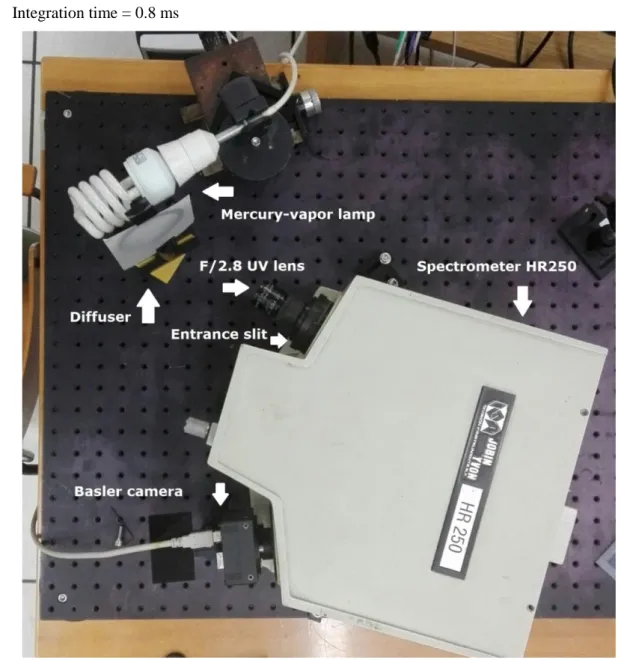
The aim of the test is to acquire and identify a set of mercury (Hg) spectra emitted by a mercury-vapor lamp, a gas discharge lamp that uses an electric arc through vaporized mercury to produce light. The main peak
65 that characterizes these spectra is located at the wavelength of 350nm. The other devices used in this test are a spectrometer HR250 and a camera Basler F312A.
The spectrometer main parameters are invariable throughout the tests: • Gain = 700
• Integration time = 0.8 ms
Figure 4 - Optical acquisition system in laboratory
In order to simulate a variable SNR in the input sets, the spectrometer’s diaphragm is adjusted at different f-number, increasing or decreasing the amount of light that passes through the lens. The f-number of an optical system is the ratio of the system’s focal length to the diameter of the aperture. We will have a greater amount of light with small values of f-number (i.e. f/2.8) and therefore a cleaner signal will be acquired. Otherwise we will have a smaller amount of light with high values of f-number (i.e. f/16) that will result in a noisy signal with poor SNR. The acquired spectra are not background-subtracted to limit error propagation.
Hence, the input set is divided in 6 subsets of spectra, each of them acquired at the following f-number value: F/2.8 - F/4 - F/5.6 - F/8 - F/11 - F/16
66
Every subset contains about 1000-1100 spectra. In each subset, 100 spectra are randomly selected and removed from it. These removed spectra will be used in the ANN test phase (600 spectra), the remaining ones (about 6000 spectra) will be used in the ANN training phase.
The SNR of every spectrum has been calculated with a ratio between the amplitude of the highest peak (in the interval of interest) and the standard deviation of a no-peak interval of the spectrum. Hence, for every subset, it has been calculated the SNR mean and the SNR standard deviation of 1000 spectra in order to have reference values that characterize each subset. The results are shown in the following table.
F/2.8
F/4
F/5.6
F/8
F/11
F/16
SNR (mean)
27,24
24,48
16,44
8,54
4,64
1,95
67 The input training set for the ANN is shown in the following image.
The target is set at the value of 1 (TRUE) for spectra with SNR-mean > 1.9 (f-number interval F/2.8 – F/11), and at the value of 0 (FALSE) for noisy spectra with SNR-mean=1.9 (f-number F/16).
68
After the training phase, the ANN is launched with each one of the test set with different f-number. The results are shown in the next classification confusion matrix.
Training
SNR=27.2 SNR=24.4 SNR=16.4 SNR=8.5 SNR=4.6 SNR=1.9
0
1
0
1
0
1
0
1
0
1
0
1
0
1
0 19 1.1
0
0
0
0
0
0
0
1
0
8
94
0
1 1 78.9 0
100
0
100
0
100 0
99
0
92
6
0
As we can see in the table above, the ANN accuracy is perfect (100%) for spectral classification with SNR>8.5.
With SNR=8.5 the net registers only a false-negative (missed hit) over 100 spectra, while at SNR=4.6 the false negatives amount raises at 8, with an overall accuracy of 92%. In these 2 subsets there are no false positives because the target values are all set to 1 (TRUE).
With SNR=1.9, hence with all targets set to 0 (FALSE), the net registers 6 false positives over 100 spectra, with an overall accuracy of 94%.
In the following images there an example of false negative spectrum and a false positive spectrum retrieved during the tests.
9 CONCLUSIONS
After these series of tests, some conclusions about the ANN performances evaluation in spectral classification tasks can be listed.
In the first section we have analyzed the impact of the input set dimension on the final neural network processing. For the simplest classification task, the input size does not appear to affect the ANN overall accuracy: an accuracy of 98.7% has been estimated from N=104 to N=105. However, the accuracy increased
69 to 99.2% with N=106. Moreover, the ANN processing time shows an exponential trend proportionally with
the input size. We started from a nearly instantaneous response with N=104 up to 5 seconds with N=105 and
9.30 minutes with N=106. Anyway, in our future experiments, we do not expect to use millions of vectors,
so, for now, the input size is not a parameter that we should worry about.
A similar conclusion can be asserted with the results of the third test where we have analyzed the impact of the hidden layer size (the number of neurons) in the network accuracy. Apparently this parameter does not seem to affect the accuracy at all, since we measured a value of 92.2% for different architectures with both higher and lower values of layer size than the default one. This can be explained with the simple nature of the tasks.
The main parameter that affects hardly the network performances for these spectral classification tasks is surely the signal to noise ratio, as it can be observed in the second test and in the following ones. In our primary task of discriminating a Gaussian signal from the noise, the accuracy is > 99% until S/N 2. Decreasing the ratio, the network accuracy starts to reduce consistently: 93.2% with S/N 1, 77.1% with S/N 0.5, 61.8% with S/N 0.2. Anyway, these can be considered as optimal results, achieving a good classification even with very low signal to noise ratios. In the more refined problem of the two Gaussian discrimination, the trend is the same, but the accuracy is lower: we have 98.6% with S/N 3, 93.5% with S/N 2 and 78.3% with S/N 1. Although it is impossible to predict a realistic S/N ratio in true spectroscopic data, these preliminary tests demonstrate the importance and the necessity to apply de-noising methods to the measured spectra in a pre-processing phase, as well, of course, as adopt all possible cares to achieve signals with the best quality (i.e. the highest S/N ratio).
Regarding to the two Gaussian tests, we already demonstrated that most part of the false positives are noise-induced peaks that fall into the interval of interest. The ANN performance, otherwise, does not seem to be affected from the presence of the second interferent Gaussian signal. This is a good promising feature for the possibility of a Raman spectral classification based on ANN: the contemporary presence of several peaks should not affect the accuracy of the ANN in the identification of a certain peak of interest.
By now, the only critical issues emerged in these tasks are the known problems of the noise that can alter the accuracy and the performance of the ANN, and the necessity to have a large number of vectors (of the order of thousands for these tests) to train the network. This last issue can be challenging in a real operating scenario.
Further work is necessary to investigate the spectral classification problem: first of all, we are going to compare the ANN performance obtained with other vector classification criteria (e.g. Euclidean distance, Correlation Coefficient, Least Squares, Absolute Different Value) and different algebraic and/or statistical methods to be searched in literature. Then, we must re-run these tests after a pre-processing phase in order to clean the signal with a correct filter (e.g. Wavelet, Savitzky-Golay filter, Wiener filter, Moving Average filter, Percentile filter). In addition, as we explained in a previous paragraph, the noise model should be improved to adapt the simulation towards a more realistic input set (Pink Noise).
70
10 REFERENCES
Taylor K., Neural Networks using MATLAB. Function Approximation and Regression. Kindle Edition, 2017. De Bernardis P., Il rumore e la sua origine fisica. Tecniche Sperimentali di Astrofisica (dispense). Università Roma “La Sapienza”, 2017.
Debska B., Guzowska-Swider B., Searching for regularities in a Raman spectral database. Journal of Molecular Structure, Elsevier 2014.
Liu J. et al, Deep Convolutional Neural Networks for Raman Spectrum Recognition: A Unified Solution. 2017 Kwiatkowski A. et al, Algorithms of chemicals detection using Raman Spectra. Metrology and Measurement Systems, 2010.
ENEA
Servizio Promozione e Comunicazione
www.enea.it
Stampa: Laboratorio Tecnografico ENEA - C.R. Frascati maggio 2019