September 10 -11 2009, Glasgow, UK
C
ALIBRATION OF A6
DOF
R
OBOTICM
ANIPULATOR BASED ON A LOW-
COSTW
IRE SENSORS MEASURING SYSTEMMonica Tiboni, Giovanni Legnani
Università degli Studi di Brescia, Brescia, Italy
Abstract: This article presents the results of a research project which aimed to investigate the applicability of wire sensors in the kinematics calibration of robotic manipulators. One indispensable operation in calibration is the measurement of the position and orientation of the robotic gripper in a predefined set of locations in the work space. For this operation high-cost sensors are generally used, such as laser tracker systems. It would seem relevant to study the possibility of using low-cost sensors, investigating the performances that it is pos-sible to obtain. With this aim, a study of simulation and experimentation was carried out on an anthropomor-phic robot with 6 revolute degrees of freedom. In the simulation phase, with the aim to optimizing calibra-tion, the influence of several parameters (number of sensors, positioning of sensors, model parameters, etc...) was studied. In the experimental phase, the efficiency of the optimized calibration procedure was verified by applying it to the real robot, achieving an accuracy close to the repeatability of the robot.
Key words: Industrial Robots, Kinematics Calibration, Wire sensors.
I I
NTRODUCTIONIn the industrial environment, the introduction of ro-botized work cells has enabled the achievement of high precision and the reduction of working hours, while increasing production flexibility. The program-ming of off-line cells is so much more widespread and strategic that it resembles dealing with a numerically controlled machine. However it is necessary that both the robot and the work cells are sufficiently accurate to obtain a real effectiveness in off-line programming. This does not always happen due to manufacturing and assembling tolerances (geometric errors), the limits of the transducers being used, the elasticity and the back-lash of the mechanical parts, the environmental condi-tions of use and the load applied. The tolerance, with which the various robot components are realized, is sometimes not able to guarantee the necessary preci-sion for the required tasks. On the other hand, the growth in constructive accuracy beyond certain limits, proves to be practically and economically prohibitive. In any case, in the majority of applications the robots are sufficiently repetitive and it is more simple and economical to correct the accuracy errors using cali-bration techniques ([1]).
Calibration requires the use of very expensive equip-ment to measure the position errors of the manipulator, such as optical sensors, which also do not always offer a sufficient range of measure. The aim of this study is to analyse, from both a theoretical and experimental point of view, the possible use in calibration of special wire transducers able to measure the length of the ca-ble when the robot gripper moves (figure 1). These
have the advantage of being much more cheaper and allow the measurement of large movement (up to some meters), with an average accuracy of (from 0.1% to 0.01% of the range of motion).
Figure 1: Calibration with wire sensors. Examples in current literature report on the application of wire sensors for the measurement of the gripper pose and of the manipulator work space, by trilatera-tion ([2]).
The robot under consideration, in both the simulation and experimentation phases, is a 6-DoF (degrees of freedom) anthropomorphic robot called DOGHI, from which a complete model of structural errors has been developed. The work carried out can be summarized into three phases: the preliminary phase, the simulation phase and the experimentation phase. In the prelimi-nary phase the plan for the measurement system was developed, identifying two possible different configu-rations for the positioning of the measurement trans-ducers and defining the parameters to describe the structural errors of the measurement system. In the simulation phases it was possible to investigate the influence of the number and location of the sensors on the calibration performances and to study the observability and eventual redundance of the parame-ters. In the experimentation phase the performances of the sensors (accuracy, repeatability and linearity) were
evaluated by connecting the wire sensors to the linear axes of a parallel-serial robot equipped with linear op-tical encoders.
Finally, the calibration of the DOGHI robot was performed by experimental measurements of its posi-tioning error and using the Newton-Raphson algorithm and an extended Kalman filter.
II T
HED
OGHIR
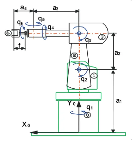
OBOTDOGHI is a 6 DOF anthropomorphic robot, powered by brushless motors and employing Harmonic Drive reducers. a1 a2 a3 a4 q1 q2 q3 q4 q5 q6 f X0 Y0 a1 a2 a3 a4 q1 q2 q3 q4 q5 q6 f X0 Y0
Figure 2: Structure of the DOGHI robot. Figure 2 displays a schematization of the robot and its geometrical parameters. Table 1 presents the nu-meric values of range of the joint rotations.
q1 270° 4.712 rad q2 124° 2.164 rad q3 112° 1.955 rad q4 360° 6.283 rad q5 210° 3.665 rad q6 360° 6.283 rad
Table 1: Range of the joint rotations of the DOGHI robot.
Figure 3: Working-space of DOGHI robot (measures expressed in mm).
Figure 3 represents the actual work space of the robot, detailing on the X1-Z1 plane its shape and size. To calibrate the robot following the parametric approach, it is necessary to develop a geometrical model of the actual robot describing all the relevant geometrical parameters λi (the structural parameters).
In general, using the formalism of the 4x4 matrices as outlined in [1], [3], [4], the theoretical position of the gripper is described by the matrix M0n:
∏
= −=
n j j j nM
M
1 , 1 0 (1)Each matrix Mj-1,j depends on a number of parameters
λi In the real robot the final position of the gripper will be different from M0n, as the matrices Mj-1,j do not as-sume their ideal value. If we indicate
M
0n the final position actually reached, its relation with the theoreti-cal position can be expressed as:j m j j n n n
M
M
M
λ
λ
∆
∂
∂
+
≅
∑
=1 0 0 0 (2)where
∆
λ
j denote the structural error. To define a valid set of structural errors there are two possible pro-cedures:1. considering a variation of the value of the parame-ters used for the kinematic description of the ma-nipulator (eg: the parameters of Denavit & Har-temberg);
2. consider the nominal values of such parameters and add others, suitably chosen, which describe the errors and assume the value zero in the ideal case.
In both cases a set of minimum, complete and propor-tional parameters should be obtained.
For the calibration of the DOGHI robot the second option has been chosen adopting the systematic method described in [3], [4] as detailed below:
• for each revolute joint it is necessary to insert two translations and two rotations around di-rections orthogonal to the motion axis of each joint.
• for the prismatic axes it is necessary to intro-duce two rotations as only the errors of orien-tation are significant, not those of positioning. • for the end-effector of the robot it is neces-sary to consider 6 parameters (3 rotations, and 3 translations) which describe its shape In the case of a robot with R revolute joints and P prismatic joints, nλ parameters are necessary, equal to
P
R
n
λ=
6
+
4
+
2
.In our case R=6 and P=0, there-fore nλ is equal to 30.For the DOGHI robot, the considered geometric pa-rameters adopted to describe the sources of error, are presented in table 2, where generic position errors are
represented as ai, bi and ci, and angular errors by αi, βi and γi.
Joint Number of
parameters Parameters descrip-tion 1 4 a1, b1,α1,β1 2 4 a2, b2,α2,β2 3 4 a3, b3,α3,β3 4 4 a4, b4,α4,β4 5 4 a5, b5,α5,β5 6 4 a6, b6,α6,β6 gripper 6 a7, b7,c7,α7,β7,γ7 Table 2: Geometric Parameters λi for the DOGHI
ro-bot.
III P
LAN FOR THEM
EASUREMENTS
YSTEMA.
Wire sensors
There exist different typologies of sensors used for calibrating robots, but they are all very expansive. The choice of wire sensors has been considered as they are much more cheaper but would however guarantee an adequate precision in measurement. According to the standards for the certification of robot performance UNI EN ISO 9283 [1], the measurement procedure must have an uncertainty of not more than 25% of the value to be verified. In our case, the value to be veri-fied being precisely the unknown quantity of calibra-tion, meant that we could only consider reliable the results not less than 25% of the maximum error of the utilized instrumentation. If we consider that the aver-age error in accuracy for anthropomorphic robots is in the order of 3-4mm [4], then to obtain a halving of the error, the entire chain of measurement must have a maximum error of less than 0.5 mm. The choice of wire transducers is very delicate because they belong to the chain of measurement.
Figures 4 and 5 present the scheme and the working principle of the wire sensors. The wire is wound on a reel, when the cable which passes trough a fix chock is pulled, the reel rotates charging a spring which main-tains the proper tension in the cable. A suitable sensor measures the rotation of the reel and so the amount of the pulled wire. The rotation can be measured by a potentiometer or, as in our case, by an incremental encoder.
The calibration of the DOGHI robot requires the use of wire transducers capable of taking measurements within the 3D space.
The search for sensors with these characteristics did not give positive outcomes. As the only available wire transducers were those for applications in which the wire works perfectly on an axis with the exit hole, or within a cone of a 20 degree width with its axis cen-tred on the exit hole, it was necessary to add a guide-wire device to the sensor. We employed a nozzle with
a calibrated hole through which passes the wire. A support plate was constructed around this nozzle to permit its suitable positioning with respect to the sen-sor to permit an easy motion of the wire.
Figure 4: Working principle of a wire transducer.
Figure 5: Wire transducer.
B. Characterization of the transducers
To investigate the performances of the wire sensors (repeatability, accuracy and linearity) they were mounted on the linear motors of a Parallel Kinematic Machines equipped with linear optical encoders (CHEOPE [5], figure 6).
Figure 6: CHEOPE parallel robot used for the charac-terization of the transducers
The movement measured by the linear encoder was used to calibrate the wire sensors. For each transducer four repetitions were carried out. The sensor was set to zero at the beginning of the first repetition. The slide was made to move along the full length of its run,
e-∆l
=R
∆α
potentiometer /encoder reel fix chock∆α
∆l
qual to 650mm, with steps of 50mm. At the end of the displacement the motion was reversed. The first and third repetitions were carried out for increasing values of movement, the second and the fourth for decreasing values. For each sensor the error of measurement ei
was calculated: i trasd i ott i
m
m
e
=
,−
, (3)where ei indicates the measurement relative to the i-th
position, mott,i the measurement of the linear optical
encoder, mtrasd,i, the measurement of the i-th
trans-ducer. For all the sensors, with the exception of the first, the error proved to be quite linear.
Figure 7: Errors of measurement for sensor 4. Figure 7, as an example, displays the measuring error of sensor 4. To achieve a good calibration of the robot it is necessary to compensate for these errors. For this reason the measuring error was approximated by a regression curve. For the first sensor a third degree polynomial was used, while for the other ones a poly-nomial of second degree was appropriate.
C.
The Arrangement of the Transducers
Another problem to be solved was the decision on where to place the wire sensors. If 6 sensors are em-ployed it is possible to measure the position and the orientation of the robot gripper. The principle is that of the 6-DOF hexapods with kinematics structure similar to Stewart-Goug platform. Knowing the location of the ends of the cables as well as their length, the pose (po-sition and orientation) of the gripper can be exactly computed. Sensor can be placed with a great freedom to respect only the given constraint regarding the maximum length of the wire. However the location of the wire sensor influences the precision of the pose estimation and so of the quality of the calibration. Sev-eral sensor locations were investigated to identify those that produce better measuring results.
Besides others two sensor configurations were selected for a deeper analysis. The first considered configura-tion uses sensors fixed to ground to a portal structure, and to a cross on the gripper (fig.8). After deciding the sensor arrangement, the second step was to decide the
exact distance between them. To optimize them we made use of the concept of isotropy, to obtain some homogenous measurements within all the work space covered by the transducers. In general, a determined quantity is isotropic if it does not vary in different di-rections. In our case it is desired to obtain measure-ments that present the same reliability independently of the point in which they were performed. We ob-served that the kinematic structure determined by the set of transducers and by the robot gripper is analo-gous with that of a PKM manipulator (Parallel Kine-matic Machine). The idea was taken from an article [6] which describes the geometric conditions that an exapod must comply with in order to obtain an iso-tropic behaviour. Following this concept the sensor disposition of Figure 9 was designed. .
Figure 8: Arrangement of the sensors in the portal con-figuration (left on ground, right on the gripper).
.
Figure 9: Arrangement of the sensors in the isotropic configuration (left on ground, right on the gripper). Having determined the most suitable arrangements for the two configurations (figures 8, 9), they were com-pared by computer simulation to select those that sup-plied the better calibration results.
From the simulations it emerged that the isotropic con-figuration of Fig. 9 is the most suitable.
D.
Parameters of the measurement system
To perform a suitable calibration of the robot it is nec-essary that the measuring system is calibrated to avoid measuring errors. This require the necessity to identify all the possible sources of errors to which the meas-urement system is subject. It is therefore indispensable to introduce parameters that properly consider the dis-crepancies between the model and reality to avoid at-tributing measurement system errors to the robot. The nominal geometry of the measurement system is described by the position of the transducers, or better by the chock hole, a point of reference with respect to which the distances are calculated, and from the posi-tion of the wire ends hooked to the robot gripper. For
each one of the points determined by the nominal ge-ometry it is necessary to introduce three possible errors δxi, δyi, δzi. We indicate by δxib, δyib, δzib the errors for the chock points and with δxig, δyig, δzig those for the wire ends. Moreover for every sensor used, it is necessary to introduce a further parameter δli (error of wire length) which considers possible off-set errors of the transducer system, or of the zero off- set-ting of the encoder. Indicaset-ting
n
Tb,
n
Tg,
n
T respec-tively the number of points fixed to ground, the num-ber of points fixed to the gripper and the numnum-ber of transducers, altogether the error parameters of the sen-sor system are equal to:T g T b T ps
n
n
n
n
=
3
+
3
+
(4) For the configuration of figure 9 where, on the gripper, the ends of the cables are connected in pair we get33
6
3
3
6
3
+
+
=
=
psn
and so the total number ofthe parameters is 33.
IV S
IMULATIONSBefore performing experiments and processing the experimental data, computer simulations were con-ducted, with the aim of evaluating and optimizing the developed algorithms.
A.
Total Parameters of the Robot-System of
Measurement Set
Paragraph 2 presents the robot model and paragraph 3 discusses the measurement system, but also the cou-pling of the two models must be analyzed with care, because some of the parameters could be redundant, others not observable. It was therefore necessary to determine a complete, minimum and proportional set of parameters describing the manipulator and the measuring system. Through observation of the posi-tioning of the reference frames and of the definition of the structural parameters, it emerged that the minimum number of geometric parameters nλ is:
8
7
4
+
−
=
R
n
Tn
λ ifn
T≥
3
(5)4
7
4
+
−
=
R
n
Tn
λ ifn
T<
3
(6) Table 4 summarizes the geometric parameters chosen for modelling the robot-measurement system set. Ta-ble 5 shows the number of structural parameters as a function of the number of sensors.B.
Observability and influence of the
pa-rameters
To study the observability of the parameters a proce-dure was applied based on the singular value
decom-position (SVD, [5],[6]) of jacobian matrices relative to the errors of position and measurement.
From the analyses carried out it emerged that none of the robot parameters have a negligible effect and so all of them have to be estimated. On the other hand, the parameters relative to the zero settings of the encoders δli and the errors for the chock points (δxib, δyib, δzib) proved to be only slightly observable.
Description Parameters number nλ ai i = 2..6 [mm] 5 bi i = 2..6 [mm] 5 αi i = 2..6 [rad] 5 βi i = 2..6 [rad] 5 x1b, z1g [mm] 2 xib, yib , zib i = 2..nT [mm] 3(nT-1) xib, yib , zib i = 2..nT [mm] 3(nT-1) dli i = 2..nT [mm] nT
Table 4: Selected geometric parameters. N° of sensors N° of parameters 1 27 2 34 3 37 4 44 5 51 6 58 Table 5: Number of parameters as a function of the
number of sensors
C. Number of transducers
From the tests carried out on varying the number of transducers, positioned in the portal configuration, and keeping constant the number and value of the consid-ered poses, it emerged that:
a. it is possible to estimate almost all the geometric parameters of the robot and of the transducers by us-ing just one sensor (except for the six that determine the geometry of the gripper, whose pose calibration needs six sensors), since the analysis based on SVD methodology carried out proved all the parameters to be observable
b. the effect of the combined parameters becomes more visible and easier to assess with the increase of the number of sensor.
Subsequently the influence of the number of the con-sidered poses on the result was investigated and it emerged that: with the same number of transducers, there is a slight improvement in observability by using a greater number of poses; such improvement is more evident when there is a low number of sensors; the improvement that can be obtained by increasing the number of considered poses is not comparable with
that achievable by increasing the number of transduc-ers.
D. Arrangement of the transducers
After having evaluated the influence of the number of transducers, the impact of their arrangement was ana-lysed. In particular the two arrangements, portal and isotropic, were compared. To be able to carry out the comparison, both the number of sensors, equal to 6, and the number of measuring poses, equal to 50, were kept constant. The isotropic arrangement produced more observable parameters than the portal one.
E. Calibration
Before analyzing the experimental data, simulations were performed to the calibration procedure; the aim was the check the correct functioning of the imple-mented algorithms. To verify the performances three indices were used, defined as follows:
( )
(
S mis)
T
RMS
T
L
T
E
=
−
( )
(
pos S posreal)
Spos
RMS
S
L
S
E
=
−
,( )
(
rot S rotreal)
Srot
RMS
S
L
S
E
=
−
, (7)Ls=[λ1, λ l2, .. λ li,...]t is the vector containing the
structural parameters to be identified by minimizing the following errors:
ET: average quadratic value of the transducer error; ESpos: average quadratic value of the error of the
fi-nal position of the robot gripper;
ESrot: average quadratic value of the error of the final
orientation of the robot gripper;
where T(LS) is the measurement of the wire lengths
computed with the estimated parameters, Tmis is the
sensor reading (measure) simulated by the transducers,
Spos(LS) e Srot(LS) are the position and orientation of
the gripper calculated with the estimated parameters,
Spos,real e Srot,real are the real position and orientation of
the gripper and RMS(.) is the average quadratic value.
Sensors n° 6 5 4 3 2 1 ET
[ m ] N-R 1.2e-12 5.2e-15 5.6e-13 1.6e-12 6.7e-13 1.9e-12 K 3.0e-06 2.2e-06 1-4e-06 1.3e-06 9.7e-07 8.2e-07 ESpos
[m] N-R 3.9e-12 1.9e-14 6.7e-13 1.3e-12 1.59e-12 2.8e-12 K 1.1e-05 3.1e-06 1.3e-06 1.4e-06 1.1e-06 1.0e-06 ESrot
[rad] N-R 5.2e-12 1.4e-14 1.1e-12 1.1e-12 1.6e-12 2.9e-12 K 1.2e-05 1.1e-05 6.6e-06 5.9e-06 4.4e-06 3.7e-06
Table 6: Performance indices’ values in simulation Table 6 shows the values of the errors, in dependence of the number of sensors varying from one to six, with
the two algorithms. It was observed that the procedure allows the estimation of the value of the parameters with an accuracy close to that of the calculator, even in the case where only one transducer was used.
For the estimation of the parameters two algorithms were implemented (after comparing their effectiveness for the problem under examination): Newton-Rhapson and an extended Kalman filter
Figure 10 cites, for example, ESpos at variation with the
configuration (where 1,2,...,6 represent portal configu-ration with respectively 1,2,..6 sensors, while ISO rep-resents the isotropic configuration with 6 sensors). The vertical segments indicate the range of error evaluated in the different tests, while the points display the average value of the error. It may be seen that both the range and the average value decrease as long as the number of sensors increase. The isotropic configura-tion with six sensors achieved the best result.
Figure 10: Values of ESpos at variance with the con-figuration
V P
RACTICALE
XPERIMENTATIONThe experimental phase of the project was sub-divided into three steps: tests for the characterization of the robot, for the characterization of the sensors, and fi-nally, calibration tests. For this purpose it was decided to use 6 wire sensors to better estimate all the parame-ters of the manipulator (figure 11).
Figure 11: DOGHI Robot fitted out with the measure-ment system.
A. Repeatability of the robot
The estimation of the repeatability of the DOGHI ro-bot was performed in accordance with the UNI EN ISO 9293 standard and, as indicated by the standard, the monodirectional repeatability (RP) and repeatabil-ity of multidirectional positioning (vAP) were esti-mated.
It resulted that the positioning repeatability RP was a little less than 1 mm and the orientation repeatability was about 5 mrad. The variation in the accuracy for multidirectional positioning vAPP were a little less than 3 mm and 7 mrad.
B. Repeatability of the sensors
The experimental verification of the sensors perform-ances (section IIIB and figure 7) shown that their re-peatability is about 0.1 mm.
Simulations were performed to verify its influence in the measure of the gripper pose. The simulation were performed by a MATLAB script that estimate the gripper position starting from the wire length; the re-peatability of the sensors was simulated by adding random value in the range 0-0.1mm to the wire length. It was verified that the error in the estimation of the gripper pose is of the same order.
This means that an amplification effect of the errors does not exist.
C. Calibration
The calibration was performed by moving the manipu-lator to different poses forming a 3D grid contained in the manipulator working space.
To select the most suitable points to form the grid a simulation was performed. A grid with 102 points was selected (Figure 12).
Figure 12: Grid of points used for the robot calibration. Indicating with T the vector containing the experimen-tal measures (the wire lengths) and with Ls the set of the structural parameters, the grid of point was opti-mized in order to improve the singular values of the jacobian matrix J (
J
=
∂
T
∂
L
s ).Different set of grid point were tested, for each set was calculated the corresponding jacobian, the singular values of each jacobian were calculated by the SVD (singular value decomposition) algorithm. The set with the higher value of the singular values were selected.
In fact a low value of one or some singular values in-dicates that the corresponding parameters cannot be estimated with good accuracy.
The 102 data collected during experimentation was called 'complete set'. The complete set was divided in two groups of data: 'the calibration set' and the 'control set'. The calibration set was used to perform the esti-mation of the structural parameters, while the control set was used to check the quality of the results. The estimation procedure was repeated three times, using different dimensions for the calibration set and the control set:
a. 50 poses of calibration, 52 poses of control; b.80 poses of calibration, 22 poses of control; c. 102 poses of calibration, no control poses. To evaluate the quality of calibration the index ET (average error) was used as introduced in paragraph 4; the maximum error between predicted Ts and
meas-ured Tr wire length was also evaluated:
(
ri si)
T
T
T
E
max=
max
,−
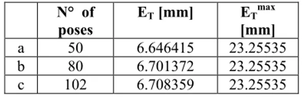
, i=1,2,..,np (8) where np is the number of considered measurements. The accuracy of the robot before calibration was evaluated with the same indices ET and ETmax (table 7). The calculations were carried out using the nominal value of the geometric parameters. The results ob-tained after calibration for the different groups of posi-tions are presented in table 8.
By comparing the error before (Table 7) and after (Ta-ble 8) calibration, it quite evident that the error was notably reduced, obtaining accuracy close to the re-peatability of the robot.
N° of poses ET [mm] ETmax [mm] a 50 6.646415 23.25535 b 80 6.701372 23.25535 c 102 6.708359 23.25535 Table 7: Values of the indices of error before
calibra-tion.
Cal.set/control set Alg. Error Value
ET [mm] 1.485/2.155 N-R ETmax[mm] 4.485/11.50 ET [mm] 1.776/2.380 50/52 K E Tmax[mm] 7.337/11.246 ET [mm] 1.718/1.645 N-R E Tmax[mm] 8.251/6.072 ET [mm] 1.977/2.146 80/22 K ETmax[mm] 9.481/11.214 ET [mm] 1.682/- N-R ETmax[mm] 8.583/- ET [mm] 1.932/- 102/- K ETmax[mm] 10.225/-
VI C
ONCLUSIONSThe presented study shows how it is possible to obtain a valid system of calibration at a low cost by using wire transducers. Proof of its effectiveness is the im-provement in accuracy obtained for an anthropomor-phic robot with 6 degrees of freedom, the DOGHI ro-bot. From an initial phase of simulation, it emerged that, although 6 transducers are necessary for a com-plete measurement of the position, a single sensor is enough to calibrate the robot (excluding the gripper shape). In every case, a higher number of sensors per-mits the achievement of a greater precision in calibra-tion. An isotropic arrangement of the transducers was also determined which seemed to guarantee the reduction of the error at the minimum theoretical value. The simulation showed that the adoption of a suitable subgroup of geometric parameters can im-prove the convergence of the algorithms. Some auto-matic procedures able to remove parameters unneces-sary to the calibration were implemented. Their adop-tion in the experimental tests confirmed the usefulness of an algorithm for parameter selection to improve calibration.
R
EFERENCES[1] G. Legnani. Robotica Industriale. Casa Editrice Ambrosiana, Milano, 2003.
[2] E. Ottaviano. M. Ceccarelli, M. Toti, C. Avila Carrasco. CATRASYS (Cassino Tracking System):
a wire system for experimental evaluation of robot workspace. Fuji Int. Journ. of Robotics and
Mechatronics, Vol.14, No.1: 78-87, 2002.
[3] G. Legnani. Robotica Industriale. Casa Editrice Ambrosiana, Milano, 2003.
[4] D. Tosi, G. Legnani. Calibration of a Parallel-Serial Hybrid Redundant Manipulator. Proceed-ings of the ROBOT&VISION SHOW-ISR 2003, Chicago, 2-5 June, 2003.
[5] Giovanni Legnani, D. Tosi, G. Ziliani, N. Pedroc-chi, Cheope: a 7 Degree of Freedom Reconfigur-able Parallel-Serial Hybrid Redundant Manipula-tor, ISR2005 36th Int. Symposium on Robotics, 29-11/1-12/2005, Keidanren kaikan Tokyo, Japan. [6] Fassi I., Legnani G., Tosi D., Geometrical Condi-tions for the Design of Partial or Full Isotropic Hexapods J. of Robotic Systems 22(10), 507-518 (2005). DOI: 10.1002/rob.20074
[7] B.W. Mooring, Z.S. Roth, M.R. Driels. Funda-mentals of manipulator calibration, New York, 1991.
[8] R. Adamini, A. Omodei, G. Legnani. Three methodologies for the calibration of industrial manipulators: experimental results on a SCARA robot, Journal of Robotic System 17(6), pp. 291-307, Wiley, 2000.
[9] G. Legnani, J.P. Trevelyan. Static calibration of industrial manipulators: a comparison between two methodologies, Robotics Toward 2000 Twenty-Seventh Int Symp on Industrial Robots, pp. 111-116, Oct. 6-8, 1996.
[10] J. Zierteg, P. Datseris, Basic considerations for robot calibration, Int J Robot Automat 4(3), 1989, pp.158-166.
[11] A. Nowrouzi, Y.V. Kavina, H. Kochekali, R.A. Whitaker, An overview of robot calibration tech-niques, Ind Robot (UK), pp. 229-232, 15(4), 1988.
![Figure 1: Calibration with wire sensors. Examples in current literature report on the application of wire sensors for the measurement of the gripper pose and of the manipulator work space, by trilatera-tion ([2])](https://thumb-eu.123doks.com/thumbv2/123dokorg/5507729.63608/1.892.528.708.609.701/figure-calibration-examples-literature-application-measurement-manipulator-trilatera.webp)