UNIVERSITY
OF TRENTO
DIPARTIMENTO DI INGEGNERIA E SCIENZA DELL’INFORMAZIONE
38050 Povo – Trento (Italy), Via Sommarive 14
http://www.disi.unitn.it
MAPPING LARGE-SCALE KNOWLEDGE ORGANIZATION
SYSTEMS
Fausto Giunchiglia, Dagobert Soergel, Vincenzo Maltese and
Alessandro Bertacco
May 2009
Technical Report # DISI-09-029
Also: in the proceedings of the 2nd International Conference on the
Semantic Web and Digital Libraries (ICSD), 2009
Mapping large-scale Knowledge Organization Systems
Fausto Giunchiglia *, Dagobert Soergel **, Vincenzo Maltese *, Alessandro Bertacco *
* Dipartimento di Ingegneria e Scienza dell’Informazione (DISI), Università di Trento {fausto, maltese, bertacco}@disi.unitn.it
** College of Information Studies, University of Maryland [email protected]
Abstract. Identifying semantic correspondences between vocabularies is a fun-damental step towards enabling interoperability among them. In this paper we report the results of a matching experiment we conducted between two large scale knowledge organization systems, i.e. NALT and LCSH. We show that, even if there is still large scope for improvements, automatic tools can signifi-cantly reduce the time necessary at finding and validating correspondences. Keywords: Knowledge Organization Systems, interoperability, mappings
1 Introduction
This paper presents a concept-based approach to automatic mapping between Knowledge Organization Systems (KOS), and describes its concrete instantiation to the mapping between the Library of Congress Subject Headings (LCSH) and the US National Agricultural Library Thesaurus (NALT) as an example.
To achieve semantic interoperability between different KOS one must establish semantic correspondences, called mappings, between their terms/concepts. This is a hard problem since vocabularies differ in structure (e.g. thesauri, classifications, for-mal ontologies), reflect different visions of the world (different conceptualizations), contain different terminology and polysemous terms, have different degrees of speci-ficity, scope and coverage, can be expressed in different languages and so on. Many projects have dealt with mappings between KOS, for example the German CARMEN1, the EU Project Renardus [15], and OCLC initiatives [16]. One possible
approach is to exploit mappings from a reference scheme, or spine, to search and na-vigate across a set of satellite vocabularies. For instance, Renardus and HILT [17] use DDC. Some others prefer LCSH [23, 24]. Both manual and semi-automatic solutions are proposed. A recent paper [14] focusing on the agricultural domain compares the two approaches and concludes that automatic procedures can be very effective but tend to fail when background knowledge is needed. Approaches to this problem have been proposed in [17, 8]. Yet it is clear that automatic approaches require manual va-lidation and augmentation of computed mappings (see for instance [19], which also describes a tool that supports this task). [2, 5, 12, 20] provide a good survey of the
state of the art on mapping computation. In particular, the OAEI2 initiative [20] aims
at providing an evaluation of such kind of tools.
In this paper we present the results of a matching experiment conducted as part of the Interconcept project, a collaboration between the University of Trento, the Uni-versity of Maryland, and the U.S. National Agricultural Library (NAL). The main goal of the project is to test the prototype of a novel concept-based system developed at the University of Trento which identifies the minimal mapping, as formalized in [8]. Minimal mappings are very effective in visualization, validation and maintenance tasks. We report the results of the matching conducted between NALT and LCSH. We show that the automatic parsing of the KOS structures can identify problems and imprecisions which are really difficult or nearly impossible to identify by manual in-spection, such as duplicated entries, cycles, and redundant relations. In addition, we show that current matching results can be improved by enhancing the NLP pipeline and by improving the quality and coverage of the available background knowledge.
The rest of the paper is organized as follows. Section 2 provides the notion of mi-nimal and redundant mappings and briefly describes how to compute them. Section 3 introduces the experiment, its main goals and steps. Section 4 lists the main experi-ment results in terms of difficulties encountered while Section 5 provides and com-ment matching results. Section 6 concludes the paper by drawing some conclusions and providing future directions.
2 Minimal and redundant mappings
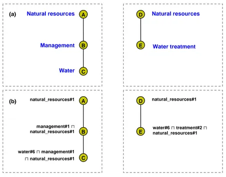
KOS usually describe their content using natural language labels, which is useful in manual tasks (e.g. for document indexing) but not for automatic reasoning (for in-stance for automatic indexing and matching) or when dealing with multiple languag-es. Therefore, we use NLP techniques tuned to short phrases [21] to translate natural language labels, exactly or with a certain degree of approximation, into their formal alter-ego, namely into lightweight ontologies [9, 10]. Lightweight ontologies, or for-mal classifications, are tree structures where each node label is a language-independent propositional Description Logic (DL) formula codifying the meaning of the node. Taking into account its context (namely the path from the root node), each node formula is subsumed by the formula of the node above. Thus, the backbone structure of a lightweight ontology is represented by subsumption relations between nodes. Look at Fig. 1 (a) for an example of two classifications and at Fig. 1 (b) for the corresponding lightweight ontologies. Natural language labels from the original sources are translated into the corresponding formulas. Each constituent concept is designated by a term from WordNet followed by the sense number; for instance, water#6 designates “a liquid necessary for the life of most animals and plants”.
In our experiments we use the MinSMatch algorithm [8]. MinSMatch takes two lightweight ontologies in input and finds those nodes in the two structures which se-mantically correspond to one another. Any such pair of nodes, along with the seman-tic relationship holding between the two, is what we call a mapping element. Possible semantic relationships computed by the algorithm are disjointness (⊥), equivalence (≡), more specific (⊑) and less specific (⊒). Over this set a partial order is imposed,
such that disjointness is stronger than equivalence which, in turn, is stronger than sub-sumption (in both directions), and such that the two subsub-sumption symbols are unor-dered. Notice that under this ordering there can be at most one mapping element be-tween two nodes.
Fig. 1. Two classifications (a) and corresponding lightweight ontologies (b) MinSMatch returns the minimal mapping, i.e. the minimal subset of mapping ele-ments from which all the others can be efficiently computed from them in time linear with the size of the two lightweight ontologies. Elements which can be computed from the minimal set are said to be redundant. More specifically, a mapping element m’ is redundant w.r.t. another mapping element m if the existence of m’ can be as-serted simply by looking at the positions of its nodes w.r.t. the nodes of m in their re-spective ontologies. In algorithmic terms, this means that a redundant mapping ele-ment can be computed without running computational expensive reasoning tools, such as SAT [8]. With this goal, four basic redundancy patterns, one for each semantic re-lation, are identified. They are shown in Fig. 2. Here, straight solid arrows represent minimal mapping elements, dashed arrows represent redundant mapping elements, and curves represent redundancy propagation. For instance, taking any two paths in the two ontologies, a minimal subsumption mapping element is an element with the highest node in one path whose formula is subsumed by the formula of the lowest node in the other path (see pattern 1). The minimal mapping is the set of mapping elements with maximum size without redundant mapping elements. Notice that for any two given lightweight ontologies, the minimal set always exists and it is unique. A proof of this statement is provided in [8].
Natural resources Natural resources
Water treatment Management Water A B C D E (a) natural_resources#1 natural_resources#1 water#6 ⊓ treatment#2 ⊓ natural_resources#1 management#1 ⊓ natural_resources#1 water#6 ⊓ management#1 ⊓ natural_resources#1 A B C D E (b)
Fig. 2. Redundancy detection patterns
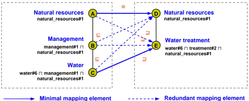
Fig. 3 provides the minimal mapping and the mapping of maximum size (including the mazimum number of redundant elements) computed between the lightweight on-tologies in Fig. 1. Original natural language labels are shown for ease of comprehen-sion. The mapping of maximum size can be efficiently computed on demand by propagation of the elements in the minimal mapping [8]. For instance, the element <B, E, ⊒> is obtained by propagation of <C, E, ⊒> by applying pattern 2. Notice that here we assume the axiom treatment#2 ⊑ management#1 to be present in the back-ground knowledge.
Fig. 3. The minimal mapping between two lightweight ontologies
The minimal mapping offers clear advantages for visualization and validation. Given two lightweight ontologies of sizes n and m, it is not feasible to visualize and validate even a small subset of all possible n x m mapping elements. Not surprisingly, the interfaces offered by current tools have scalability problems in their visualization and management [19, 22]. Minimal mappings are a very small portion of the overall mapping elements between the two KOS, making manual validation much easier, faster, and less error-prone [13]. If an element is positively validated, all its derived mapping elements are correct; on the other hand, if it is negatively validated we can-not conclude anything about the correctness of its derived redundant mapping
ele-A B C D (1) ⊑ ⊑ A B (2) C D ⊒ ⊒ A B C (3) D ⊥ C D E F (4) A B ≡ ≡ ⊥ ≡
Minimal mapping element Redundancy propagation
Redundant mapping element
⊑ ⊒ ≡ Natural resources natural_resources#1 Natural resources natural_resources#1 Water treatment water#6 ⊓ treatment#2 ⊓ natural_resources#1 Management management#1 ⊓ natural_resources#1 Water water#6 ⊓ management#1 ⊓ natural_resources#1 ⊑ ⊒ ⊒ A B C D E
ments. Each redundant element, therefore, must be considered separately. However, a partial order, as defined in [8] (see the theorem on minimal mapping, existence and uniqueness), can be enforced on the set of its derived mapping elements. Under this ordering we can identify the maximal elements in the set (which can be said to be sub-minimal) and iterate the process. For instance, in case the element <A, D, ≡> is not correctly validated, the maximal elements in the set {<A, E, ⊒>, <B, D, ⊑>, <C, D, ⊑>} of its derived redundant mapping elements are <A, E, ⊒> and <B, D, ⊑>. The mapping element <C, D, ⊑> needs to be validated only in case <B, D, ⊑> is not posi-tively validated.
3 The experiment
Our approach is concept-based; we use advanced linguistic techniques to automati-cally express terms from a KOS as propositional Description Logic (DL) formulas and then we use such formulas to compute the minimal mapping between the nodes in the KOS. Rather than evaluating the mapping found, i.e. in terms of precision/recall, the main goal of the project is to learn from errors and understand how to progressive-ly improve the matching process. We report the results of a matching experiment we conducted between NALT and LCSH:
• NALT (US National Agriculture Library Thesaurus) 2008 version containing 43037 subjects, mainly about agriculture, which are divided in 17 subject cate-gories (e.g.. Taxonomic Classification of Organisms, Chemistry and Physics, Bi-ological Sciences). NALT was available as a text file formatted to make rela-tionships recognizable.
• LCSH (US Library of Congress Subject Headings) 2007 version containing 339976 subjects in all fields. LCSH was available in the MARC 21 format en-coded in XML.
In both KOS the records are unsorted and the information about the hierarchical structure is implicitly codified in the relations between preferred terms.
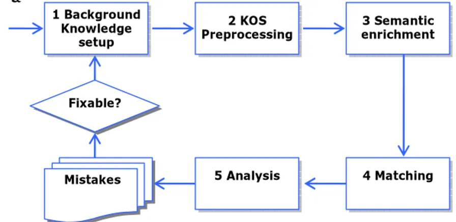
The matching experiment has been organized in a sequence of 5 steps (Fig. 4) which can be iterated to progressively improve the quantity and the quality of the mapping elements found. From the analysis of the node formulas and the mapping elements computed by the algorithm, at each iteration problems and mistakes can be identified and fixed. In Step 1, Background Knowledge setup, WordNet was im-ported; in Step 2, KOS preprocessing, the two KOS were parsed and converted into classifications and in Step3, semantic enrichment, they were translated into lightweight ontologies; finally, in Step 4, Matching, MinSMatch was executed to compute the minimal mapping between them. The analysis step concludes the process.
In the following we provide additional details about single steps performed: Step 1. Background Knowledge Setup. The availability of an appropriate amount of background knowledge is clearly fundamental for any application which deals with semantics. It is also self evident that the quantity and the quality of the mapping ele-ments identified by the algorithm depend on the quality and the coverage of available
knowledge. In our framework, knowledge is stored in a Background Knowledge (BK) component which is conceptually split into two parts:
• the natural language dictionary, codifying terms, their description (glosses), senses and lexical relations between them, in multiple languages;
• the ontological part, codifying language-independent concepts and semantic re-lations between them.
We initially used WordNet to populate the BK. WordNet is a fairly large English lexical database which contains nouns, verbs, adjectives and adverbs grouped into synsets (groups of synonyms). Synsets are interlinked by conceptual-semantic and lexical relations. Version 2.1 contains 147252 unique terms grouped into 117597 syn-sets.
Fig. 4. A global view of the phases of the experiment
Step 2. Preprocessing: from KOS to classifications. During this step, the KOS are parsed and approximated to classifications using only preferred terms and BT/NT (Broader Term/Narrower Term) relations to compute tree structures.
Step 3. Semantic enrichment: from classifications to lightweight ontologies. The goal of this step is to encode the classifications, output of the previous step, into lightweight ontologies. As described in [9, 10], natural language labels are translated into propositional DL formulas. This process is also called semantic enrichment. We used a standard NLP pipeline [21], consisting of tokenization, part-of-speech (POS) tagging, and word sense disambiguation (WSD). It applies a finite set of BNF3 based
rules (derivation rules) which cover a finite set of patterns obtained by training the pipeline on DMoz4.
Step 4. Matching: Using the tree structures and the DL formulas at each node, we run MinSMatch to compute the minimal mapping and the mapping of maximum size. Step 5. Analysis of mistakes. The analysis identifies problems in each single step and fixes them if possible. The process can be iterated to further improve the results.
3 http://www.garshol.priv.no/download/text/bnf.html 4 http://www.dmoz.org/ 1 Background Knowledge setup 2 KOS
Preprocessing 3 Semantic enrichment
4 Matching 5 Analysis
Mistakes Fixable?
4 Experiment difficulties
The whole process was iterated only once. In this section we summarize and com-ment on the main results of the expericom-ment in terms of difficulties encountered and their quantitative analysis. In particular, we discuss problems of the sources, loss of information, problems due to the NLP pipeline and missing background knowledge. 4.1 Problems with the sources
We have identified the following problems/imprecisions in the KOS structures: • Ambiguous preferred terms. Both in NALT and LCSH, preferred terms are
directly used as indexes to define relations between entries (e.g. Geodesy BT Geophysics). However, lexically equivalent terms might represent a potential source of ambiguities. In LCSH there are 575 cases where the same preferred term is used in different records, for example Computers, Film trailers, Period-icals, Christmas, Cricket etc…
• Cycles. In LCSH we have found 6 chains of terms forming cycles. For instance: #a Franco-Provencal dialects BT #a Provencal language #x Dialects BT #a Provencal language BT #a Franco-Provencal dialects.
• Redundant BTs. We discovered several redundant BTs, namely distinct chains of BTs (explicitly or implicitly declared) with same source and target. For in-stance, in NALT the following chains were identified:
life history BT biology BT Biological Sciences life history BT Biological Sciences
sprouts (food) BT vegetables BT plant products sprouts (food) BT plant products
Table 1 provides some statistics about the amount of BTs and redundant BTs in NALT and LCSH. It also provides information about the number of parsed terms and the number of cases in which we have multiple non redundant BTs (i.e., a polyhie-rarchy) for a given node. These results show that automatic parsing provides clear added value with respect to manual inspection. In fact, these problems (identified dur-ing the parsdur-ing phase) are really difficult or nearly impossible to identify manually. They also give some clue about the quality of the sources. In NALT almost 2% of the BTs are redundant, while in LCSH this quantity reaches 3%.
NALT LCSH
Preferred terms imported 43038 335701 Total number of BTs 46400 344796 Multiple non redundant BTs 2821 87395
Redundant BTs 807 9256
4.2 Loss of information
The output of the parsing phase are directed acyclic graph (DAG) structures in which node labels are the preferred terms appearing in the original sources. Table 1 provides the number of preferred terms, and therefore of nodes, in the two graphs. They have to be further reduced to classifications. With this goal, we preliminary re-move redundant BTs. The remaining BTs are analyzed to identify cases of multiple BTs with same source. For each of them we keep only one BT (for instance, giving priority to those which lead to main headings) and remove all the others. After remov-ing redundant BTs and selectremov-ing one of multiple BTs (for ease of processremov-ing), both NALT and LCSH appear as a forest of trees where node labels are the preferred terms of the original NALT/LCSH records, as follows:
• LCSH: 65744 trees The 25 most populated trees include 196723 nodes (58%), 59105 trees have only one node (18% of all nodes);
• NALT: All nodes are linked to a Subject Category5 (e.g. Animal Science and
Animal Products, Biological Sciences), so we have 17 trees.
For each KOS we introduced a dummy root node (TRUE) to create a large tree. During this phase we have a clear loss of information, in particular in the kind of rela-tionships selected (we keep only BTs and NTs), in the terms selected (we keep only preferred terms) and structural information (we remove multiple BTs).
4.3 NLP problems
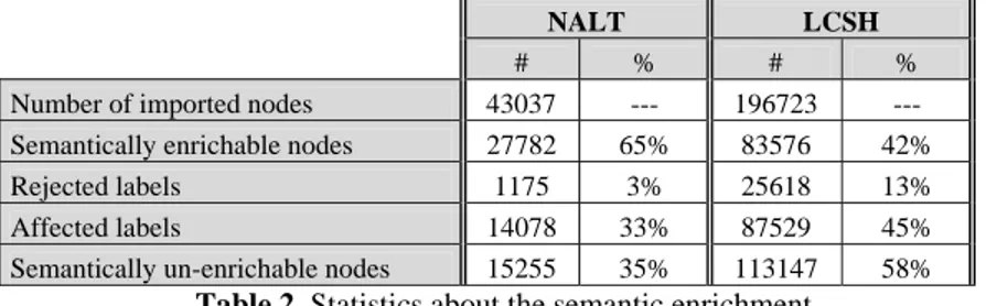
Table 2 summarizes some statistics about the quantity (#) and percentage (%) of labels which can be processed by the current NLP pipeline. Look at Table 3 for some examples of such node labels and corresponding formulas (taking into account the full path). Concepts without the number (for instance anti_corrosives#, which is also rec-ognized as a multiword) are evidence of lack of background knowledge (see next paragraph). Notice that for the properties of the lightweight ontologies, a failure in the enrichment of a node propagates to the whole subtree rooted in it. Label of nodes in such subtrees are what we call affected labels. Nodes which cannot be enriched are clearly skipped during the matching phase.
NALT LCSH
# % # %
Number of imported nodes 43037 --- 196723 --- Semantically enrichable nodes 27782 65% 83576 42%
Rejected labels 1175 3% 25618 13%
Affected labels 14078 33% 87529 45%
Semantically un-enrichable nodes 15255 35% 113147 58% Table 2. Statistics about the semantic enrichment
From Table 2 we can note that the un-enrichable nodes are a significant portion of the total number. This is particularly evident in LCSH where more than half of the la-bels are not enrichable. By analyzing the lala-bels which are not supported by the current
NLP pipeline, we identified some recurrent patters. Specifically, labels including round parenthesis, such as Life (Biology), and labels including ‘as’, such as brain as food are not currently enrichable. These kinds of labels are very frequent in thesauri. The term in parenthesis, or after the ‘as’, is used to better describe, disambiguate or contextualize terms. In particular, in NALT and LCSH, labels of the first kind are mainly used:
• to provide the acronym of a term - “Full term (Acronym)” - or to provide the full description of an acronym - “Acronym (Full term)”. For instance, nitrate reductase (NADH);
• to disambiguate homonyms. E.g., mercury (planet) and mercury (material); • to represent a compound concept, for instance, growth (economics) (which
could also be represented as economic growth).
Notice that 83% of label rejections in LCSH and the 30% in NALT are due to the missing parenthesis pattern. The pattern with ‘as’ is less frequent and represents around the 1% of the rejection cases, both in NALT and LCSH. The pipeline could be, therefore, significantly improved by including new rules for these patters. How-ever, this use of parenthesis is typical in thesauri but it is not in web directories (e.g. DMoz). It is clear that a rule based pipeline cannot cover all the cases and work uni-formly when dealing with different kinds of sources. We are working on an extended NLP pipeline which gets around all these problems.
LCSH label (and path) DL formula
Water repellents
(Chemicals / Repellents / Water repellents)
chemicals#34600 ⊓ repellents#1626 ⊓ (water#75538 ⊓ repellents#1626) Neutron absorbers
(Chemicals / Bioactive compounds / Poisons / Neutron absorbers)
chemicals#34600 ⊓ (bioactive# ⊓ compounds#84901) ⊓
poisons#23087 ⊓ (neutron#27237 ⊓ absorbers#95684) Stress corrosion
(Chemicals / Chemical inhibitors / Corrosion and anti-corrosives / Stress corrosion)
chemicals#34600 ⊓
(chemical#21081 ⊓ inhibitors#93475) ⊓ (corrosion#67669 ⊔ anti_corrosives#) ⊓
(Stress#66019 ⊓ corrosion#67669) Table 3. Some examples of labels from LCSH which can be successfully enriched 4.4 Missing background knowledge
As already underlined, the quality and the quantity of the correspondences identi-fied by the algorithm directly depend on the quality and the coverage of available knowledge. This is confirmed by recent studies, in particular for what concerns lack of background knowledge [17, 14]. Our experiment also confirms this hypothesis. In fact, we found that the 30% of the logic formulas computed for LCSH and the 72% for NALT contain at least one concept which is not present in our background know-ledge. The fact that the phenomenon is more evident in NALT is most likely because NALT is more domain specific.
To increase the quantity of knowledge we could import it from a selection of knowledge sources. We analyzed two possible candidates, the Alcohol and Other Drugs Thesaurus6 (AOD) and the Harvard Business School Thesaurus7 (HBS).
How-ever, we found that the increment of the pure syntactic (surface) overlap of the new terms (including preferred and non-preferred terms) with NALT and LCSH would be less than 0.5%. This is something not unexpected, since the reason of this discourag-ing result is probably the different focus of the thesauri: NALT is mainly about agri-culture, while AOD is about drugs and HBS is about business. This is also confirmed by a very low syntactic overlap between NALT and AOD (7%) and between NALT and HBS (4%). However, AOD and HBS are partially faceted and contain many gen-eral conceptual primitives that would be useful in a deeper semantic analysis but that would not be detected as matches at the surface level. Domain related thesauri, like AGROVOC, are also needed.
5 Matching results
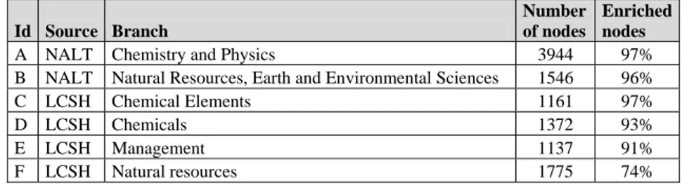
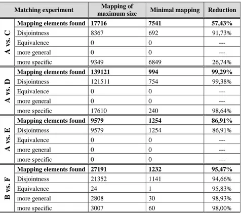
We have executed MinSMatch on a selection of NALT/LCSH branches which turned out to have a high percentage of semantically enrichable nodes. See Table 4 for details. Table 5 shows evaluation details about conducted experiments in terms of the branches which are matched, the number of elements in the mapping of maximum size (obtained by propagation from the elements in the minimal mapping), the number of elements in the minimal mapping and the percentage of reduction in the size of the minimal set w.r.t. the size of the mapping of maximum size.
Id Source Branch
Number of nodes
Enriched nodes
A NALT Chemistry and Physics 3944 97%
B NALT Natural Resources, Earth and Environmental Sciences 1546 96%
C LCSH Chemical Elements 1161 97%
D LCSH Chemicals 1372 93%
E LCSH Management 1137 91%
F LCSH Natural resources 1775 74%
Table 4. NALT and LCSH branches used
We have run MinSMatch both between branches with an evident overlap in the topic (A vs. C and D, B vs. F) and between clearly unrelated branches (A vs. E). As expected, in the latter case we obtained only disjointness relations. This demonstrates that the tool is able to provide clear hints of places in which it is not worth to look at in case of search and navigation. All the experiments show that the minimal mapping contains significantly less elements w.r.t. the mapping of maximum size (from 57% to 99%). Among other things, this can incredibly speed-up the validation phase. It also shows that exact equivalence is quite rare. We found just 24 equivalences, and only one in a minimal mapping. This phenomenon has been observed also in other projects, for instance in Renardus [15] and CARMEN.
6 http://etoh.niaaa.nih.gov/aodvol1/aodthome.htm 7 http://hul.harvard.edu/ois/ldi/
Matching experiment Mapping of
maximum size Minimal mapping Reduction
A vs
. C
Mapping elements found 17716 7541 57,43%
Disjointness 8367 692 91,73% Equivalence 0 0 --- more general 0 0 --- more specific 9349 6849 26,74% A vs. D
Mapping elements found 139121 994 99,29%
Disjointness 121511 754 99,38%
Equivalence 0 0 ---
more general 0 0 ---
more specific 17610 240 98,64%
A vs. E
Mapping elements found 9579 1254 86,91%
Disjointness 9579 1254 86,91% Equivalence 0 0 --- more general 0 0 --- more specific 0 0 --- B v s. F
Mapping elements found 27191 1232 95,47%
Disjointness 21352 1141 94,66%
Equivalence 24 1 95,83%
more general 2808 30 98,93%
more specific 3007 60 98,00%
Table 5. Results of matching experiments
6 Conclusions and future directions
In this paper we have presented the results of a matching experiment we conducted between two large scale knowledge organization systems: NALT and LCSH. We have shown that, automatic tools (even if they need to be further improved) are prom-ising and can significantly reduce the time necessary at finding and validating map-ping elements. The next steps will include investigations about how to increment the quantity and quality of the background knowledge, how to enhance the NLP pipeline, and how to assist the user in the visualization, navigation, validation and long term maintenance of the mapping found.
References
1. M. L. Zeng, L. M. Chan, 2004. Trends and Issues in Establishing Interoperability Among Knowledge Organization Systems. Journal of the American Society for Information Sci-ence and Technology, 55(5), pp: 377-395.
2. P. Shvaiko, J. Euzenat, 2007. Ontology Matching. Springer-Verlag New York, Inc. Secau-cus, NJ, USA.
3. F. Giunchiglia, M. Yatskevich, P. Shvaiko, 2007. Semantic Matching: algorithms and im-plementation. Journal on Data Semantics, IX, 2007.
4. F. Giunchiglia, M. Yatskevich, and E. Giunchiglia, 2005. Efficient semantic matching. In Proceedings of the 2nd European semantic web conference (ESWC’05), Heraklion. 5. P. Shvaiko, J. Euzenat, 2005. A Survey of Schema-based Matching Approaches. Journal on
Data Semantics, (IV) pp. 146–171.
6. F. Giunchiglia and M. Yatskevich, 2004. Element level semantic matching. In Proceedings of Meaning Coordination and Negotiation workshop at ISWC 2004.
7. F. Giunchiglia and P. Shvaiko and M. Yatskevich, 2005. S-Match: an algorithm and an im-plementation of semantic matching. In proc. of Semantic Interoperability and Integration. 8. F. Giunchiglia, V. Maltese, A. Autayeu, 2008. Computing minimal mappings. University
of Trento, DISI Technical Report.
9. F. Giunchiglia, M. Marchese, I. Zaihrayeu, 2007. Encoding Classifications into Lightweight Ontologies. Journal of Data Semantics 8, pp. 57-81.
10. F. Giunchiglia, I. Zaihrayeu, 2008. Lightweight Ontologies. To appear in Encyclopedia of Database Systems, Springer Verlag, 2008.
11. F. Giunchiglia, P. Shvaiko, M. Yatskevich, 2005. Semantic schema matching. In: On the move to meaningful internet systems 2005: coopIS, DOA, and ODBASE: OTM Confede-rated International Conferences, vol. 1, pp. 347-365.
12. P. Shvaiko, J. Euzenat, 2008. Ten Challenges for Ontology Matching. In Proc. of the 7th International Conference on Ontologies, DataBases, and Applications of Semantics. 13. C. Meilicke, H. Stuckenschmidt, A. Tamilin, 2008. Reasoning support for mapping
revi-sion. Journal of Logic and Computation, 2008.
14. B. Lauser, G. Johannsen, C. Caracciolo, J. Keizer, W. R. van Hage, P. Mayr, 2008. Com-paring human and automatic thesaurus mapping approaches in the agricultural domain. Proc. Int’l Conf. on Dublin Core and Metadata Applications.
15. T. Koch, H. Neuroth, M. Day, 2003. Renardus: Cross-browsing European subject gateways via a common classification system (DDC). In I.C. McIlwaine (Ed.), Subject retrieval in a networked environment. Proceedings of the IFLA satellite meeting held in Dublin - IFLA Information Technology Section and OCLC, pp. 25–33.
16. D. Vizine-Goetz, C. Hickey, A. Houghton, R. Thompson, 2004. Vocabulary Mapping for Terminology Services”. Journal of Digital Information 4(4)(2004), Article No. 272. 17. D. Nicholson, A. Dawson, A. Shiri, 2006. HILT: A pilot terminology mapping service with
a DDC spine. Cataloging & Classification Quarterly, 42 (3/4). pp. 187-200.
18. F. Giunchiglia, P. Shvaiko, M. Yatskevich, 2006. Discovering missing background know-ledge in ontology matching. Proceedings of the 17th European Conference on Artificial In-telligence (ECAI 2006), pp. 382–386.
19. S. Falconer, M. Storey, 2007. A cognitive support framework for ontology mapping. In Proceedings of ISWC/ASWC, 2007.
20. C. Caracciolo, J. Euzenat, L. Hollink, R. Ichise, A. Isaac, V. Malaisé, C. Meilicke, J. Pane, P. Shvaiko, 2008. First results of the Ontology Alignment Evaluation Initiative 2008. 21. I. Zaihrayeu, L. Sun, F. Giunchiglia, W. Pan, Q. Ju, M. Chi, and X. Huang, 2007. From
web directories to ontologies: Natural language processing challenges (ISWC 2007). 22. G. G. Robertson, M. P. Czerwinski, J. E. Churchill, 2005. Visualization of mappings
be-tween schemas. In Proc. of the SIGCHI Conf. on Human Factors in Computing Systems. 23. C. Whitehead, 1990. Mapping LCSH into Thesauri: the AAT Model. In Beyond the Book:
Extending MARC for Subject Access, pp. 81.
24. E. O'Neill, L. Chan, 2003. FAST (Faceted Application for Subject Technology): A Simpli-fied LCSH-based Vocabulary. World Library and Information Congress: 69th IFLA Gen-eral Conference and Council, 1-9 August, Berlin.