A QUANTILE REGRESSION APPROACH FOR MODELLING A HEALTH-RELATED QUALITY OF LIFE MEASURE
Giulia Cavrini
0. IN MEMORY OF ANTONIO PARMEGGIANI
With sincerity and affection, I would like to dedicate this work to the memory of Professor Antonio Parmeggiani, whose intellect and wisdom continues to in-spire me. My Master Professor during my thesis and again for my PhD, he was not only a guide to my scientific growth but a stimulating, warm, friendly, amiable and cheerful person. His delightfully dry sense of humor, his benevolence and integrity and his scientific rigor and wise counsel are deeply missed.
1. INTRODUCTION
Measuring the health of the population is important for guiding policy deci-sions in public health. Health policy is usually aimed at improving health and re-ducing socioeconomic health differences. Consequently, both the level and the distribution of health provide relevant information for setting and evaluating goals in public health policy (Hoeymans et al., 2005).
Morbidity and mortality are often used to indicate the general health of a population. Another important outcome of health in clinical, intervention and epidemiological studies is the Quality of Life (QoL) of individuals. Quality of Life can be viewed as a subjective, multidimensional concept, which places emphasis on the self-perception of an individual’s current state (Fayers and Machin, 2000; Bonomi, 2000). There is no consensus on a definition of QoL, although there is considerable agreement among experts that it encompasses social and psycho-logical well-being as well as health status. The World Health Organization (WHO, 1948) has declared health to be “a state of complete physical, mental and social well-being, and not merely the absence of disease”. Many other definitions of both “health” and “quality of life” have been attempted, often linking the two and, for QoL, frequently emphasising components of happiness and satisfaction with life. In the absence of any universally accepted definition, some investigators argue that most people, in the western world at least, are familiar with the
expres-sion “quality of life” and have an intuitive understanding of what it comprises (Fayers and Machin, 2000).
The term Health-Related Quality of Life (HRQoL) is often used to indicate quality of life as it relates to diseases or treatments people experience.
The importance of monitoring and evaluating health and HRQoL as perceived by the general population is increasingly emphasized. From a public health per-spective, such monitoring benefits the identification of population inequalities in health status, potentially reveals unmet needs in the community and indicates the important health promoting efforts to be initiated. Health is a complex phe-nomenon and holistic definitions encompass a multiplicity of dimensions. HRQoL has been described as the impact of health ‘on an individual’s ability to function and his or her perceived well-being in physical, mental and social do-mains of life’ (Nordlund, 2005). HRQoL is thus described in functional, objec-tively quantifiable terms, as well as in more subjective terms pertaining to how the individual feels. The monitoring of HRQoL in the general population requires generic instruments that ideally capture all-important aspects of HRQoL thereby enabling comparisons within, as well as between, populations (Nordlund, 2005).
In recent years, the QoL and HRQoL measures have gained increasing atten-tion in studies focused on obtaining informaatten-tion on populaatten-tion needs to supple-ment traditional indicators of health status. Researchers and clinicians are fre-quently interested in assessing the association between the lifestyles and the Health Related Quality of Life in population studies.
A large number of different instruments measuring HRQoL have been devel-oped and some of these, such as EQ-5D, have become increasingly popular.
Compared to other instruments, the EQ-5D has the advantage of conciseness. The EQ-5D is very short: only five questions with three possible answers (Euro-QoL Group, 1990; Kind et al., 1994; Kind, 1996: Kind et al., 1998). Although some detail may be lost, this instrument has proved suitable for describing the health status of the general population (Brooks et al., 1991; Nord, 1991; Kind et al., 1998; Johnson and Coons, 1998). The psychometric properties in terms of feasibility, coverage and discrimination of the EQ- 5D are comparable to those of other instruments (Brazier, 1993; Revick and Kaplan, 1993).
Another advantage of the EQ-5D instrument is that a health profile can be linked to an index value, also known as the utility score or the preference score. (Kind et al., 1994; Kind, 1996; Hoeymans, 2005).
The development of the EQ-5D was aimed at a health state classification through which an overall single summary index value could be derived using preferences elicited from the general population thereby enabling the calculation of Quality Adjusted Life Years (QALYs) for use in economic analyses (EuroQoL Group, 1990; Kind et al., 1994; Kind, 1996: Kind et al., 1998). Though less de-tailed, the items underlying the health state classification also give information re-garding different aspects of health. Single-summary index value instruments have the practical advantage of having to deal with only one measurement in compari-sons, while profile instruments provide a more comprehensive description of dif-ferent dimensions of health. The EQ-5D has been used in general population
health surveys as well as in specific groups of patients. The EQ-5D is easily and quickly administered and HRQoL measuring instruments maximize response rates because they are brief (Brooks et al., 2003; Cavrini et al., 2004; Collina et al., 2004; Kind et al., 2005; Pacelli et al., 2005).
The EQ-5D questionnaire is a generic measure of health status developed by the EuroQoL Group (1987) (Brooks et al., 2003; Kind et al., 1994; Kind, 1996; Kind et al., 1998). It is two pages long: on the first page there are the questions about five dimensions: mobility, self care, usual activities, pain or discomfort and anxiety or depression. Each dimension is divided into three levels of perceived problem: no problem, moderate problem or an extreme problem. On the second page there is a Visual Analogue Scale (VAS) where respondents record their per-ception of their overall health. A unique health state is defined by combining one level from each of the five dimensions. This information can be used to generate a simple health profile or be converted into a single summary index (EQ-5D in-dex) by applying scores from a set of the UK general population preference weights (UK weights being used because Italian weights are not available) (Dolan et al., 1996; Dolan et al., 1996).
This work is the result of co-operation between the Department of Statistics at the University of Bologna and the Department of Epidemiology of the Health Authority. Our main aim was to analyze data in order to provide a useful measure for the Health Authority to assess the life-style determinants of a low perception of Health Related Quality of Life. In this study the EuroQoL EQ-5D question-naire was used to achieve this aim. This is one of the first occasions that the EQ-5D questionnaire has been used in Italy to conduct a survey on a sample of the general population of two Health Authorities.
In this paper we propose a new approach for modeling the EQ-5 Dimensions. We focused on a Quantile Regression Model. Investigators have commonly used multiple linear regression or logistic regression to model the measures of HRQoL. Moreover, in this work a quantile regression approach was used to evaluate such a relationship instead of the more commonly used Ordinary Least Square (OLS) regression. OLS methods may mask some of the important asso-ciations in various segments of the outcome distribution while quantile regression offers an innovative and more concise way to capture these effects in this area of research.
Quantile regression is an econometric regression model in which specific quan-tiles (or percenquan-tiles) of the response variable are regressed on subject characteris-tics. The existence of quantile regression has been largely ignored in the Clinical and Biostatistics literature, despite being frequently used in Economics literature (Austin et al., 2005).
This methodological approach was preferred to an OLS regression because both the EQ-VAS and EQ-5D index typical distributions have a peak distribu-tion (skewed to the right) that can not be well described when using a mean-based model.
2. SURVEY DESIGN AND METHODS
We report on a cross-sectional study where a postal survey was given to a sample of 1,622 adults randomly selected from the population register of two Bo-logna Health Authorities in northern Italy. Data was collected between June 2002 and October 2002. Each subject and their personal physicians were contacted by telephone three times after the inception of the survey. If the subject refused to participate in the study, they were consequently replaced with a subject randomly selected with the same age and gender.
Exclusion criteria were: people aged less than 18 years, non permanent resi-dents in the two Health Authorities, people who were in hospital or in nursing homes during the research period and people unable to reason or understand and make decisions unaided.
A package with the SF-12 and the EQ-5D questionnaires plus an additional questionnaire on patient age, gender, marital status, education, occupation and smoking behavior was sent to the home of the sampled people. In the same ques-tionnaire some health problems such as hearing problems, vision problems, dia-betes, dialysis, treatment for anxiety/depression, headache (at least once a week) were also investigated.
The purpose of adding these questions was to study diseases and symptoms that may affect everyday life and may sometimes be unknown to the General Practitioner because they do not necessarily require an appointment or a prescrip-tion.
The subjects’ personal physicians were required to complete a questionnaire about health problems with more difficult diagnoses: treatment for hypertension, heart failure, angina, COPD, asthma, back-pain, cancer in the previous five years and stomach ulcers.
The overall response rate was 82% and the partial non-response rate was less than 5% for any variables.
Preliminary descriptive analyses (frequencies, percentages, mean and standard deviation were executed in order to describe the study sample. Inferential analysis (chi-square tests, partitioned 2 x c tables, t- tests, Kruskal-Wallis tests and ANOVA) were executed in order to assess significant association and differences between investigated variables. Furthermore, the mean and standard deviation of EQ-5D and EQ-VAS were calculated for each covariate.
To evaluate the influence of the investigated covariates on the EQ-5D index and EQ-VAS, and to assess the strength of these relations, we used a Quantile Regression Model (Koenker and Basset, 1978; Koenker, 1994; Koenker, 2005; Austin et al., 2005). We preferred this approach to an OLS (Ordinary Least Squares) regression because the distribution of the EQ-5D index and EQ-VAS is rather irregular and skewed to the right, therefore we decided to perform the analysis without any transformation of its natural scale.
2.1 The Quantile Regression Model
Quantile regression (Koenker and Basset, 1978; Koenker, 1994; Koenker, 2005; Austin et al., 2005) is an econometric regression model in which a specified conditional quantile (or percentile) of the outcome variable is expressed as a lin-ear function of subject characteristics. This is in contrast to an OLS regression, in which the mean of a continuous response variable is expressed as a linear func-tion of a set of independent or predictor variables.
The specific quantile of the outcome distribution, conditioned to the values of the predictor variables is given by
1 2 0 1 1 2 2
[ | , ,..., ] ( ) ( ) ( ) ... ( )
i
y i i ki i i k ki
Q x x x x x x (1)
where Qyi( |) denotes the –quantile of the conditional distribution of yi. Thus the regression parameter k( ) denotes how the specified quantile changes with one-unit change in xk (Koenker and Basset, 1978; Koenker, 2005). The parameter vector ( ) k is estimated solving a minimum problem (minimizing an asymmet-rically weighted sum of absolute errors), which can be formulated as linear pro-gramming problems and calculated efficiently (Koenker, 2005).
If we wish to estimate the median (50th percentile) regression model, then is
equal to 0.5 for all observations, and the coefficients are chosen so as to minimize one half the sum of the absolute deviations from the regression line. For this rea-son, median regression is also known as least-absolute deviations regression. Posi-tive residuals are weighted more heavily than negaPosi-tive residuals if one wants to model a percentile that lies above the 50th percentile, while the converse is true if
one wishes to model a percentile that lies below the 50th percentile (Austin et al.,
2005).
From a user’s perspective, quantile regression is similar to linear regression in many aspects. It can be implemented using statistical software such as STATA and R. Furthermore, quantile regression enables the use of either forward or backward model selection techniques similar to those available for multiple linear regression. Quantile regression models can include interaction terms in a manner similar to ordinary linear regression. Coefficient estimates are interpreted as the increase in a given quantile of the conditional distribution in the same way that coefficients in linear regression are interpreted as the change in the mean of the conditional distribution.
There are several advantages to the use of quantile regression. Firstly, rather than assessing how the centre of a conditional distribution varies with changes in subject characteristics, one can examine how any percentile of the conditional distribution is affected by changes in subject characteristics. By examining multi-ple percentiles of the conditional distribution of time to treatment, one can exam-ine how the entire distribution, rather than only the mean, changes with subject characteristics. It is possible that certain percentiles are more affected by subject characteristics than other percentiles are. A situation may occur in which the
magnitude of the regression coefficient is minimal for a given subject characteris-tic to one percentile of the conditional distribution, while the magnitude of the regression coefficient, for the same variable but for a different percentile, is much larger. Secondly, quantile regression models are additive. Thus, the coefficients are interpreted as the change in the given percentile of the conditional distribu-tion associated with a one-unit change in the given characteristic. Thirdly, ver-sions of quantile regression exist for censored data (Koenker, 2005; Austin et al., 2005).
The covariates included in the regression model are reported in Tables 12 and 13, with the results of the quantile regression estimation at the 25th, 50th and 75th
conditional percentile. We centered each covariate in respect to its own mean value, so that the quantile regression intercept becomes a prediction of the τth quantile of the EQ-5D index or EQ-VAS with mean values for each considered covariate.
The final model only includes variables with at least one significant coefficient in one of the three observed quantiles. Thus, the variables’ marital status and Body Mass Index (BMI) are excluded, and the following were included in the fi-nal model as categorical variables: gender, classes of age, education level, whether working, smoking habits and number of concomitant pathologies (0, 1 and 2 or more).
The p-values are reported and are considered significant if less than 0.05. All analyses were performed with STATA/SE 11.0 software (Stata Corporation, Texas, USA).
3. RESULTS
3.1 Characteristics of the respondents
The socio-demographic characteristics of the 1,497 respondents are set out in Table 1, which shows the mean and the standard deviation of the EQ-5D index and VAS for each level of the variables. 52% of the sample were female. The re-spondents had a mean age of 50.2 years (SD=18.1; range: 18-93). Almost 33% had been educated beyond 13 years of schooling but only 7% had a university de-gree. The respondents were most frequently in the white collar and blue collar workers (54.9%), married (62.1%) and never smoked (52.8%).
The health problems declared by the respondents are set out in Table 2, which shows the mean and standard deviation of the EQ-5D index and EQ-VAS for each level of the variables.
The frequency distribution of BMI classes shows a high percentage of over-weight and obese subjects (45.5%). Men had a frequency of being overover-weight that is significantly higher than in women (p<0.001). In this case, partitioned 2 x 4 ta-bles into non-independent 2 x 2 tata-bles were analysed considering an adjusted sig-nificance level ’=’/(c – 1) = 0.017, where c is the number of columns in the ta-ble (in our case 4).
The approximate prevalence of diabetes is 4% and vision and hearing prob-lems are present in 11% and 14% of the sample respectively. Almost 16% of the respondents used drugs for anxiety (most were female). 34% of the respon-dents declared having another health problem, which is set out in Table 3. The principal problems concerned the circulatory (30.6%) and musculoskeletal system (20.7%).
TABLE 1
Socio-demographic characteristics of the sample and EQ-5D index mean and standard deviation Characteristics N (%) EQ-5Dindex Mean (SD) EQ-5DVAS Mean (SD)
Gender Male 718 (48.0) 0.85 (0.18) 79.4 (15.7) Female 779 (52.0) 0.77 (0.25) 74.7 (18.6) Age (year) <20 18 (1.2) 0.90 (0.17) 83.4 (13.6) 20-29 193 (12.9) 0.90 (0.13) 85.5 (11.9) 30-39 294 (19.6) 0.88 (0.17) 84.2 (12.1) 40-49 246 (16.5) 0.85 (0.15) 81.2 (13.0) 50-59 255 (17.0) 0.81 (0.17) 77.6 (13.9) 60-69 229 (15.3) 0.79 (0.17) 70.8 (17.3) 70-79 168 (11.2) 0.65 (0.33) 62.9 (21.2) 80 94 (6.3) 0.55 (0.35) 57.0 (21.9) Education
Upon to 5 years schooling (Low education) 484 (32.3) 0.71 (0.28) 67.5 (20.2) 8 years schooling (Intermediate education) 402 (26.9) 0.81 (0.19) 78.8 (15.1) 13 years schooling (High education) 490 (32.7) 0.88 (0.16) 82.6 (13.7) University Degree (High education) 104 (7.0) 0.88 (0.15) 83.4 (11.6)
Missing value 17 (1.1) Main Activity White-collar 430 (28.7) 0.88 (0.14) 83.5 (12.1) Blue-collar 392 (26.2) 0.86 (0.15) 82.2 (13.1) Student 45 (3.0) 0.89 (0.18) 85.6 (12.0) Seeking work 25 (1.7) 0.88 (0.12) 75.2 (15.1) Housewife 170 (11.3) 0.72 (0.25) 69.5 (17.9) Retired 414 (27.7) 0.70 (0.29) 66.6 (20.6) Missing value 21 (1.4) Marital status Single 380 (25.4) 0.88 (0.16) 82.9 (14.4) Married 930 (62.1) 0.81 (0.20) 76.6 (16.8) Widowed 149 (10.0) 0.63 (0.35) 62.8 (20.5) Divorced-Separated 31 (2.1) 0.80 (0.19) 81.2 (13.7) Missing value 7 (0.5) Smoking status Never smoker 791 (52.8) 0.79 (0.26) 74.9 (19.4) Ex-smoker 259 (17.3) 0.81 (0.18) 76.1 (15.7) Current smoker 430 (28.7) 0.85 (0.17) 81.2 (13.5) Missing value 17 (1.2) Health status Excellent 77 (5.1) 0.97 (0.07) 95.3 (7.8) Very good 351 (23.4) 0.94 (0.09) 89.0 (7.9) Good 715 (47.8) 0.83 (0.15) 78.2 (11.3) Fair 245 (16.4) 0.66 (0.21) 61.2 (14.3) Poor 89 (6.0) 0.33 (0.37) 38.7 (19.3) Missing value 20 (1.3) Total 1497 0.81 (0.22) 77.0 (17.4)
TABLE 2
Health problems of the sample and EQ-5D index mean and standard deviation
Health problems N (%) EQ-5Dindex mean (SD) EQ-5DVAS mean (SD)
Body Mass Index
Underweight ( 18.5) 39 (2.6) 0.76 (0.25) 77.0 (18.8) Normal (18.5-24.9) 724 (48.4) 0.82 (0.22) 79.4 (17.1) Overweight (25-29.9) 520 (34.7) 0.81 (0.21) 75.8 (16.4) Obesity I, II, III ( 30) 162 (10.8) 0.75 (0.23) 70.4 (19.2)
Missing value 52 (3.5) Diabetes Present 59 (3.9) 0.67 (0.27) 58.8 (20.2) Absent 1423 (95.1) 0.82 (0.22) 77.7 (16.9) Missing value 15 (1.0) Vision problems Present 159 (10.6) 0.58 (0.35) 58.7 (22.3) Absent 1295 (86.5) 0.84 (0.18) 79.4 (15.0) Missing value 43 (2.9) Hearing problems Present 204 (13.6) 0.66 (0.28) 64.8 (18.9) Absent 1275 (85.2) 0.83 (0.20) 78.9 (16.4) Missing value 18 (1.2)
Drugs for anxiety
Present 233 (15.6) 0.63 (0.29) 65.5 (19.5)
Absent 1234 (82.4) 0.84 (0.19) 79.2 (15.9)
Missing value 30 (2.0)
Headache al least once a week
Present 351 (23.4) 0.70 (0.27) 72.4 (19.2) Absent 1118 (74.7) 0.84 (0.19) 78.6 (16.3) Missing value 28 (1.9) Other diseases Present 517 (34.5) 0.72 (0.26) 68.4 (18.9) Absent 980 (65.5) 0.86 (0.18) 81.5 (14.7)
# of GP visits (2 previous months)
0 589 (39.3) 0.89 (0.15) 84.5 (12.2) 1 395 (26.4) 0.84 (0.16) 79.5 (13.6) 2 239 (16.0) 0.74 (0.23) 68.9 (17.8) 3 79 (5.3) 0.77 (0.18) 67.3 (16.8) 4 60 (4.0) 0.58 (0.34) 60.1 (20.7) 5 or more visits 69 (4.6) 0.50 (0.34) 54.5 (20.5) Missing value 66 (4.4)
We categorised the variable “number of health problems” into four levels: no problem, only one problem, two problems and three or more problems.
We considered the presence of the following variable clinical conditions de-clared by respondents as health problems: diabetes, vision and/or hearing prob-lems, anxiety drug use, headache (at least once a week) and the presence of the health conditions reported in Table 3.
The categorised variable has been called “comorbidity” and its frequency and percentage distribution is set out in Table 4, which shows the mean and the stan-dard deviation of the EQ-5D index for each level of the variables. 10% of the sample declared three or more simultaneous health problems.
TABLE 3
Diagnostic group of the most common self-reported health conditions and EQ-5D index mean and standard deviation
Diagnostic group N (%) EQ-5Dindex
Mean (SD) EQ-5DMean (SD) VAS Diseases of the Circulatory System 158 (30.6) 0.70 (0.30) 67.9 (18.2) Diseases of the Musculoskeletal System 107 (20.7) 0.67 (0.23) 66.2 (20.1) Diseases of the Digestive System 54 (10.4) 0.76 (0.18) 67.1 (14.2) Diseases of the Respiratory System 28 (5.4) 0.72 (0.21) 61.6 (20.0)
Neoplasm 24 (4.6) 0.71 (0.20) 59.4 (18.1)
Diseases of Thyroid 23 (4.4) 0.77 (0.26) 80.1 (11.0)
Diseases of the Genitourinary System 22 (4.3) 0.70 (0.29) 70.5 (17.6) Allergies and Psoriasis 22 (4.3) 0.88 (0.13) 84.2 (12.0) Diseases of the Blood 20 (3.9) 0.89 (0.12) 78.0 (13.9) Diseases of the Nervous System 18 (3.4) 0.57 (0.45) 58.9 (25.2)
Anxiety/Depression 4 (0.8) 0.59 (0.41) 70.5 (14.8)
Other diagnostic group 37 (7.2) 0.78 (0.21) 70.6 (22.2)
Total 517 (100.0)
TABLE 4
Comorbidity and EQ-5D index mean and standard deviation
Comorbidity N (%) EQ-5Dindex mean (SD)
No health problem 568 (37.9) 0.92 (0.11)
Only one problem 463 (31.0) 0.81 (0.18)
Two problems 240 (16.0) 0.73 (0.20)
Three or more problems 151 (10.1) 0.52 (0.34)
Missing value 75 (5.0)
3.2 Self-reported health status
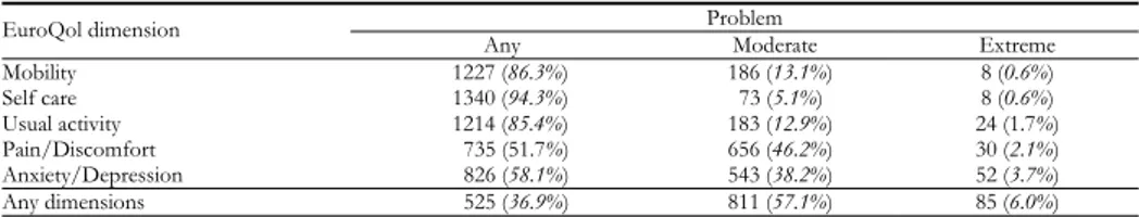
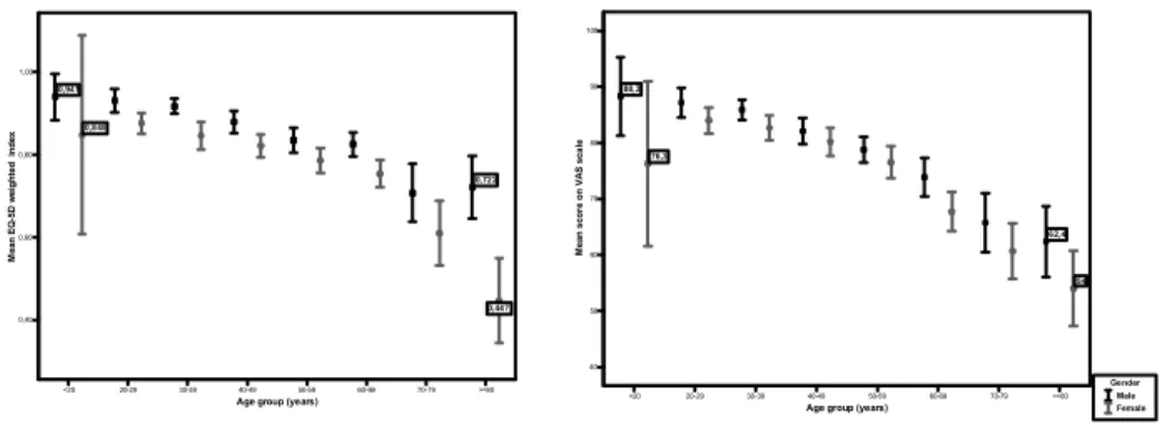
Table 5 shows the rates of reported problems on EQ-5D dimensions. A mod-erate problem on at least one dimension was reported by 57.1% of respondents, whereas only 6.0% of respondents reported any extreme problem. Problems were most often recorded in the pain or discomfort dimension (46.2%). A high per-centage of people declaring a moderate problem in anxiety or depression dimen-sion (38.2%) was revealed. 811 respondents reported a moderate problem in at least one dimension and 85 reported an extreme problem (6.0%). The mean health state recorded on the visual analogue scale was 77 (SD 17.4). The mean Visual Analogue Scale value decreases from about 83 in the youngest age group (<20 years) to 57 in the oldest age group (80) (Figure 1). Mean values did not differ significantly in young adults (20 to 49 age range) but decreased significantly for respondents aged 50 (p<0.0001).
TABLE 5
Rates of reported problem on EQ-5D dimensions Problem EuroQol dimension
Any Moderate Extreme
Mobility 1227 (86.3%) 186 (13.1%) 8 (0.6%) Self care 1340 (94.3%) 73 (5.1%) 8 (0.6%) Usual activity 1214 (85.4%) 183 (12.9%) 24 (1.7%) Pain/Discomfort 735 (51.7%) 656 (46.2%) 30 (2.1%) Anxiety/Depression 826 (58.1%) 543 (38.2%) 52 (3.7%) Any dimensions 525 (36.9%) 811 (57.1%) 85 (6.0%)
<20 20-29 30-39 40-49 50-59 60-69 70-79 >=80 Age group (years)
0,40 0,60 0,80 1,00 M ea n E Q -5 D w eight ed inde x 0,941 0,722 0,848 0,447 <20 20-29 30-39 40-49 50-59 60-69 70-79 >=80
Age group (years) 40 50 60 70 80 90 100 M ean sco re o n V A S sca le 88,3 62,4 76,3 54 Gender Male Female
Figura 1 – Mean and 95% confidence interval for self-rated health status of respondents.
A category of age has been created for highlighting the association between age group, gender, marital status, educational level, BMI group, smoking status and comorbidity.
Women aged 40 tended to report significantly higher rates of problems than men of the same age (Table 6). A systematic difference in rates was found across all age groups on the anxiety/depression dimension, with women reporting sig-nificantly higher rates than men (p<0.01). A statistically significant difference was found in the VAS scores for men and women, for age group (p< 0.0001) and for interaction gender-age (p<0.05): this is valued with an ANOVA with two fixed factors.
Perceived health status, measured with EQ-5D index and VAS scale, was worse for women than men in all age groups.
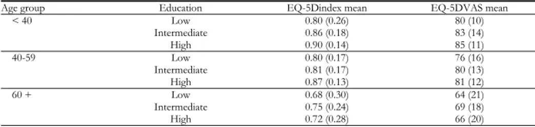
Respondents who were widowed (Table 7) and those with low education levels (Table 8) reported significantly more problems in all five dimensions (p<0.0001).
Overweight and obese respondents present significantly lower EQ-5D index and VAS values than normal weight subjects (Table 9 and Figure 2).
TABLE 6
EQ-5D index mean and VAS mean for gender and age group
Age group Gender EQ-5Dindex mean EQ-5DVAS mean
< 40 Men 0.92 (0.12) 86 (11)
Women 0.86 (0.18) 83 (13)
40-59 Men 0.86 (0.16) 80 (13)
Women 0.80 (0.16) 78 (14)
60 and over Men 0.77 (0.22) 69 (19)
Women 0.64 (0.32) 62 (21)
TABLE 7
EQ-5D index mean and VAS mean for gender, age group and marital status
Age group Marital status EQ-5Dindex mean EQ-5DVAS mean
< 40 Single 0.90 (0.14) 85 (12) Married 0.84 (0.18) 84 (12) Widowed 0.79 (0.08) 50 (-) Divorced-Separated 0.91 (0.12) 87 (8) 40-59 Single 0.84 (0.18) 77 (16) Married 0.83 (0.16) 80 (13) Widowed 0.85 (0.12) 78 (10) Divorced-Separated 0.73 (0.20) 79 (15) 60 + Single 0.71 (0.22) 61 (24) Married 0.73 (0.24) 67 (19) Widowed 0.60 (0.36) 64 (21) Divorced-Separated 0.87 (0.21) 79 (17) TABLE 8
EQ-5D index mean and VAS mean for gender, age group and education
Age group Education EQ-5Dindex mean EQ-5DVAS mean
< 40 Low 0.80 (0.26) 80 (10) Intermediate 0.86 (0.18) 83 (14) High 0.90 (0.14) 85 (11) 40-59 Low 0.80 (0.17) 76 (16) Intermediate 0.81 (0.17) 80 (13) High 0.87 (0.13) 81 (12) 60 + Low 0.68 (0.30) 64 (21) Intermediate 0.75 (0.24) 69 (18) High 0.72 (0.28) 66 (20) TABLE 9
EQ-5D index mean and VAS mean for BMI class
BMI group EQ-5Dindex mean EQ-5DVAS mean
Underweight ( 18.5) 0.76 (0.25) 77 (19)
Normal (18.5-24.9) 0.82 (0.22) 79 (17)
Overweight (25-29.9) 0.81 (0.21) 76 (16)
Obesity I (30-34.9) 0.76 (0.23) 72 (19)
Obesity II and III ( 35) 0.71 (0.23) 67 (20)
Mean VAS values are significantly lower in the smokers group (Table 10) with respect to non-smokers (75) and ex-smokers (76) (Table 10).
TABLE 10
EQ-5D index mean and VAS mean for Smoking status
Smoking status EQ-5Dindex mean EQ-5DVAS mean
Never smoked 0.79 (0.26) 75 (19)
Ex-smoker 0.81 (0.18) 76 (16)
Current smoker 0.85 (0.17) 81 (13)
Subjects reporting no problem in any dimension have high EQ-5D index and EQ-5D VAS means. These values tend to decrease if subjects declare having one or more health problems. In particular, the EQ-5D index mean dropped to 0.52 in subjects with three or more health problems and the EQ-5D VAS mean falls to 57. Controlling for comorbidity and age, gender is the most important variable affecting perceived health status.
BMI and health status are strictly connected to comorbidity. If they do not present comorbidity, obese subjects declare a better health status than those of a normal weight. Obese subjects with one or more health problems present lower EQ scores with respect to people of a normal weight.
TABLE 11
EQ-5D index mean and VAS mean for comorbidity
Comorbidity EQ-5Dindex mean EQ-5DVAS mean
No health problem 0.92 (0.11) 86 (11)
Only one problem 0.81 (0.18) 77 (15)
Two problems 0.73 (0.20) 69 (17)
Three or more problems 0.52 (0.34) 57 (20)
3.3 The quantile regression results
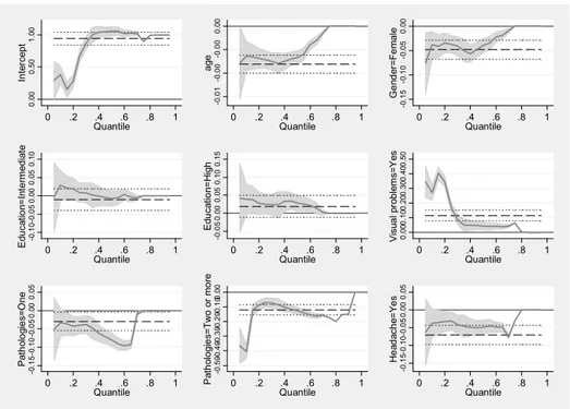
Table 12 shows the results from the quantile regression analysis using the EQ-5D index as the outcome variable. A more concise visual summary of the results is provided in Figure 3. The solid line represents the quantile regression line and the shaded area the 95% confidence interval. Superimposed on the plot is a dashed line representing the ordinary least squares (OLS) estimate of the mean effect with the dotted lines representing its 95% confidence interval. In the first panel of the figure, the intercept of the model may be interpreted as the condi-tional quantile function of the EQ-5D index distribution of a mean age of 50 years, female, with a low education level, with no vision problems, no headache problems and with no pathology, in general.
The increase in age and the differential effect for gender were only significant for the lower quantiles (25th and 50th); younger males having higher values
com-pared to females. Even a higher education did not seem to increase the quality of life, except in the 50th quantile. As expected, the presence of headache problems
per-ceived quality of life. This disparity was especially high for two or more patholo-gies with coefficients -0.07 in the 25th, -0.13 the 50th, and -0.16 in the 75th
percen-tile, respectively. Unexpectedly, being overweight or obese compared to not being overweight was not associated with perceived quality of life in any quantile. Fi-nally, being a smoker compared to a non smoker was not associated with the EQ-5D index.
TABLE 12
Quantile regression estimates for EQ-5D index
Coef. SE t p-value (95% CI)
25th quantile Age -0.0028 0.0004 -6.47 0.000 (-0.0037 – -0.0020) Gender Female -0.0374 0.0114 -3.27 0.001 (-0.0598 – -0.0150) Education level Intermediate 0.0092 0.0130 0.71 0.477 (-0.0162 – 0.0347) High 0.0256 0.0149 1.72 0.086 (-0.0036 – 0.0549) Visual problems Yes 0.1698 0.1396 1.22 0.224 (-0.1040 – 0.4436 Headache Yes -0.0315 0.0108 -2.91 0.004 (-0.0527 – -0.0103) Pathologies One -0.0402 0.0108 -3.74 0.000 (-0.0614 – -0.0191) Two or more -0.0703 0.0149 -4.72 0.000 (-0.0996 – -0.0411) Constant 0.6704 0.2897 2.31 0.021 (0.1020 – 1.2388) 50th quantile Age -0.0027 0.0005 -5.40 0.000 (-0.0037 – -0.0017) Gender Female -0.0395 0.0098 -4.02 0.000 (-0.0588 – -0.0223) Education level Intermediate -0.0069 0.0153 -0.45 0.650 (-0.0369 – 0.0230) High 0.0279 0.0143 1.96 0.051 (-0.0001 – 0.0559) Visual problems Yes 0.0442 0.0209 2.12 0.034 (0.0033 – 0.0851) Headache Yes -0.0489 0.00847 -5.77 0.000 (-0.0656 – -0.0323) Pathologies One -0.0797 0.0184 -4.33 0.000 (-0.1158 – -0.0436 ) Two or more -0.1266 0.0161 -7.84 0.000 (-0.1583 – -0.0323) Constant 1.0578 0.0628 16.83 0.000 (0.9345 – 1.1811) 75th quantile Age -0.0006 0.0006 -1.04 0.299 (-0.0017 – 0.0005) Gender Female -0.0093 0.0096 -0.97 0.333 (-0.0280 – 0.0095) Education level Intermediate -0.0058 0.0129 -0.45 0.654 (-0.0312 – 0.0196) High 0.0017 0.0084 0.21 0.835 (-0.0147 – 0.0181) Visual problems Yes 0.0445 0.0233 1.91 0.056 (-0.0012 – 0.0902 Headache Yes -0.0758 0.0344 -2.21 0.028 (-0.1433 – -0.0084) Pathologies One -0.0093 0.0282 -0.33 0.743 (-0.0647 – 0.0461) Two or more -0.1561 0.0232 -6.73 0.000 (-0.2016 – -0.1105 ) Constant 1.0222 0.0805 12.70 0.000 (0.8643 – 1.1812)
0. 00 0. 50 1. 00 In te rc ep t 0 .2 .4 .6 .8 1 Quantile -0 .0 1 -0 .0 0 -0 .0 0 0. 00 ag e 0 .2 .4 .6 .8 1 Quantile -0 .1 5 -0 .1 0 -0 .0 5 0. 00 G e nd er = F e m a le 0 .2 .4 .6 .8 1 Quantile -0 .1 0 -0 .0 5 0. 00 0. 05 0. 10 E du cat io n= Int e rm ed iat e 0 .2 .4 .6 .8 1 Quantile -0 .0 5 0. 00 0. 05 0. 10 0. 15 E du cat io n= H igh 0 .2 .4 .6 .8 1 Quantile 0. 00 0. 10 0. 20 0. 30 0. 40 0. 50 V is ua l pr ob le m s=Y es 0 .2 .4 .6 .8 1 Quantile -0 .1 5 -0 .1 0 -0 .0 5 0. 00 0. 05 Pa th ol o gi e s= O n e 0 .2 .4 .6 .8 1 Quantile -0 .5 0-0 .4 0-0 .3 0-0 .2 0-0 .1 00. 00 P ath ol og ie s= T w o o r m o re 0 .2 .4 .6 .8 1 Quantile -0 .1 5-0 .1 0-0 .0 5 0. 00 0. 05 H e ad ac h e= Y e s 0 .2 .4 .6 .8 1 Quantile
Figura 3 – Point estimates and 95% confidence intervals from a quantile regression of the EQ-5D
index distribution.
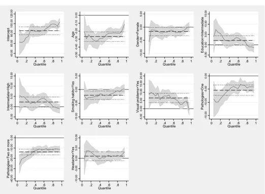
In Table 13 and Figure 4 the results from the quantile regression for the EQ-VAS as outcome variable are reported. The results were similar to those obtained for the EQ-5D index, except for the smoking habits variable. The effect of gen-der was only statistically significant for the high quantiles consigen-dered (75th). As in
the previous analyses, men had a better overall perceived quality of life. As ex-pected, age was statistically and negatively significant for all quantiles. As in the previous case, BMI was not significant and not considered in the final model. It is important to highlight that the smoking habits variable, not significant for the EQ-5D index, is significant for VAS; it has a particularly negative effect on the lower quantiles (25th and 50th percentiles). Vision problems and the presence of
one or two or more pathologies was negatively associated with the VAS in all quantiles; in particular, the presence of two or more pathologies is associated with a decrease in VAS of 17, 11 and 11 points in the 25th, 50th and 75th quantiles
TABLE 13
Quantile regression estimates for EQ-5D VAS
Coef. SE t p-value (95% CI)
25th quantile Age -0.3061 0.03023 -10.13 0.000 (-0.3654 – -0.2468) Gender Female -1.4898 1.2511 -1.19 0.234 (-3.9443 – -0.9647) Education level Intermediate 3.8367 1.8744 2.05 0.041 (0.1595 – 7.5140) High 2.7755 1.8889 1.47 0.142 (-0.9302 – 6.4812) Smoking habits Yes -2.7959 0.9880 -2.83 0.005 (-4.7342 – -0.8577) Visual problems Yes 9.3673 2.3132 4.05 0.000 (4.8292 – 13.9055) Headache Yes 2.1224 2.0423 1.04 0.299 (-1.8842 – 6.1291) Pathologies One -7.8367 1.6027 -4.89 0.000 (-10.9809 – -4.6925) Two or more -16.7143 2.6734 -6.25 0.000 (-21.9592 – -11.4694) Constant 74.3878 6.6726 11.15 0.000 (61.2970 – 87.4785) 50th quantile Age -0.2778 0.04821 -5.76 0.000 (-0.3724 – -0.1832) Gender Female -1.4167 0.9487 -1.49 0.136 (-3.2779 – 0.4446) Education level Intermediate 2.4722 1.2802 1.93 0.054 (-0.0394 – 4.9838) High 3.3333 1.3976 2.39 0.017 (0.5914 – 6.0753) Smoking habits Yes -2.2222 0.8206 -2.71 0.007 (-3.8322 – -0.6122) Visual problems Yes 8.3611 2.2797 3.67 0.000 (3.8886 – 12.8336) Headache Yes 0.1111 1.7595 0.06 0.950 (-3.3408 – 3.5630) Pathologies One -4.0278 1.3182 -3.06 0.002 (-6.6140 – -1.4416 ) Two or more -10.8333 1.8084 -5.99 0.000 (-14.3811 – -7.2856) Constant 84.0556 6.5154 12.90 0.000 (71.2733 – 96.8378) 75th quantile Age -0.2222 0.0317 -7.01 0.000 (-0.2844 – -0.1601) Gender Female -2.0741 0.8557 -2.42 0.015 (-3.7528 – -0.3953) Education level Intermediate -1.6296 1.2958 1.26 0.209 (-0.9125 – 4.1717) High 1.4074 1.4247 0.99 0.323 (-1.3877 – 4.2026) Smoking habits Yes -0.7407 0.5624 -1.32 0.188 (-1.8440 – -0.3626) Visual problems Yes 2.5926 1.4682 1.77 0.078 (-0.2878 – 5.4730) Headache Yes 1.0740 0.7290 1.47 0.141 (-0.3561 – 2.5042) Pathologies One -3.6267 0.8632 -4.20 0.000 (-5.3231 – -1.9362) Two or more -11.1852 1.1632 -9.62 0.000 (-13.4673 – -8.9031 ) Constant 98.5556 3.9242 25.11 0.000 (90.8567 – 106.2544)
40 .0 0 60 .0 0 80 .0 0 10 0 .00 1 20. 00 In te rc ep t 0 .2 .4 .6 .8 1 Quantile -0 .5 0 -0 .4 0 -0 .3 0 -0 .2 0 -0 .1 0 0. 0 0 Ag e 0 .2 .4 .6 .8 1 Quantile -1 0 .0 0 -5 .0 0 0. 0 0 5. 00 G end er = F em a le 0 .2 .4 .6 .8 1 Quantile -5 .0 0 0. 00 5. 00 10 .0 0 15 .0 0 E d uc at io n = In te rm ed ia te 0 .2 .4 .6 .8 1 Quantile -5 .0 0 0. 0 0 5. 0 0 10 .0 0 15 .0 0 In te rm ed ia te = H ig h 0 .2 .4 .6 .8 1 Quantile -1 0 .0 0 -5 .0 0 0. 0 0 5. 0 0 Sm ok in g h abi ts = Y es 0 .2 .4 .6 .8 1 Quantile -5 .0 0 0. 0 0 5. 0 0 10 .0 0 15 .0 0 20 .0 0 V is u al pr o bl em s= Y es 0 .2 .4 .6 .8 1 Quantile -1 5 .0 0 -1 0. 00 -5 .0 0 0. 0 0 Pat hol og ie s= O ne 0 .2 .4 .6 .8 1 Quantile -4 0 .0 0 -3 0 .0 0 -2 0 .0 0 -1 0 .0 0 0. 0 0 Pat hol og ie s= T w o o r m or e 0 .2 .4 .6 .8 1 Quantile -1 0 .0 0 -5 .0 0 0. 0 0 5. 0 0 10 .0 0 H e ad ac he = Y e s 0 .2 .4 .6 .8 1 Quantile
Figura 4 – Point estimates and 95% confidence intervals from a quantile regression of the EQ-5D
VAS distribution.
4. CONCLUSIONS
In this paper we propose a new approach for modelling the “EQ-5D index” and the EQ-VAS. Quantile regressions estimate several slopes, from the mini-mum to maximini-mum response, providing a more complete picture of the relation-ship between variables which are not found in other regression models.
The quantile regression objective function is a weighted sum of absolute devia-tions, which gives a robust measure of location so that the estimated coefficients vector is not sensitive to outlier observations on the dependent variable.
When the error term is not-normal, quantile regression estimators may be more efficient than least square estimators.
For regression models with heterogeneous variance (that is, a model in which the covariates’ effect changes according to the different parts of the Y distribu-tion), focusing exclusively on change in the mean may underestimate, overesti-mate or fail to distinguish real non zero changes.
In this paper we argue that quantile regression is an efficient instrument to model these measures in spite of its unusual distribution, enabling deeper investi-gation of the effects of covariates, not only on the mean, but also on the whole index and VAS distribution. The expected result of the analysis is that if we want
to obtain improvements in the quality of life of the general population we have to improve its health condition.
Department of Statistics GIULIA CAVRINI
University of Bologna
ACKNOWLEDGEMENTS
The Health Authorities of Bologna found this project. For this part of the project I thank Dr. Paolo Pandolfi MD, Dr. Natalina Collina MD, Dr. Francesca Mezzetti MD, Dr. Vincenza Perlangeli MD, Health Authority of Bologna, Dr. Barbara Pacelli, Dr. Andrea Mattivi, Emilia-Romagna Region, who preciously contributed to the data collection. A heartfelt thank you to person and physicians for accepting to participate in the study: without their help this work should have been impossible.
REFERENCES
P.C. AUSTIN, J.V. TU, P.A. DALY, D.A. ALTER(2005)The use of quantile regression in health care research : a case study examining gender differences in the timeliness of thrombolytic therapy, “Statistics in Medicine”, 24, pp. 791-816.
A.E. BONOMI, D.L. PATRICK, D.M. BUSHNELL, M. MARTIN(2000),Validation of the United States’ ver-sion of the World Health Organization Quality of Life (WHOQOL) instrument,“Journal of Clinical Epidemiology”. 53, pp. 1-12.
J. BRAZIER, N. JONES, P. KIND(1993),Testing the validity of the Euroqol and comparing it with the SF-36 health survey questionnaire, “Quality of Life Research”, 2, pp. 169-180.
R.G. BROOKS, S. JENDTEG, B. LINDGREN, U. PERSSON, S. BJORK(1991), EuroQoL: health-related qual-ity of life measurement. Results of the Swedish questionnaire exercise, “Health Policy” 18, pp. 25-36.
R. BROOKS(1996),EuroQol: The current state of play, “Health Policy”, 37, pp. 53-72.
R. BROOKS, R. RABIN, F. DE CHARRO(2003),The measurement and valuation of health status using EQ-5D: a European perspective, Kluwer Academic Publisher, The Netherlands.
M. BUCHINSKY(1998),Recent advances in quantile regression model: a practical guideline for empirical research, “The Journal of human resources”, 33, pp. 88-126.
G. CAVRINI, B. PACELLI, P. PANDOLFI, N. COLLINA, F. MEZZETTI, P. PESCI, V. PERLANGELI(2004), Modeling EQ-5 dimensions for the purposes of identifying perceived health impact of life-style determi-nants, Proceeding of 21st Scientific Plenary Meeting of the EuroQoL Group, pp. 29-44. N. COLLINA, P. PANDOLFI, F. MEZZETTI, B. PACELL, G. CAVRINI(2004),Salute percepita e salute
misu-rata. Indagine sulla qualità della vita percepita in relazione allo stato di salute nella popolazione dei Distretti Pianura Est e Pianura Ovest, Report printed by Department of Health Authority . P. DOLAN, C. GUDEX, P. KIND, A. WILLIAMS (1996), The Time Trade-off Method: Results from a
Geneeral Population Study, “Health Economics”, 15, pp. 141-154.
P. DOLAN, C. GUDEX, P. KIND, A. WILLIAMS (1996), Valuing health states: A comparison of methods, “Journal of Health Economics”, 15, pp. 209-231.
EUROQOL GROUP(1990).EuroQoL – a new facility for the measurement of health-related quality of life, “Health Policy”, 16, pp. 199-208.
P.M. FAYERS, D. MACHIN (2000), Quality of Life. Assessment, Analysis and Interpretation, Wiley, England.
N. HOEYMANS, H. VAN LINDERT, G.P. WESTERT (2005),The health status of the Dutch population as assessed by the EQ-6D, “Quality of Life Research”, 14, pp. 655-663.
J.A. JOHNSON, S.J. COONS(1998),Comparison of the EQ-5D and SF-12 in an adult US sample, “Quality of Life Research”, 7, pp. 155-166.
J.A. JOHNSON, S.J. COONS, A. ERGO, G. SZAVA-KOVATS(1998),Valuation of EuroQoL (EQ-5D) health states in an adult US sample, “Pharmacoeconomics”, 13, pp. 421-433.
P. KIND, C. GUDEX, P. DOLAN, A. WILLIAMS(1994),Practical and methodological issues in the develop-ment of the EuroQoL: the York experience, “Adv Medical Sociol”, 5, pp. 219-253.
P. KIND(1996)The EuroQoL instrument: an index of health-related quality of life. In: Spilker B, ed. “Quality of Life and Pharmacoeconomics in Clinical Trials”, 2nd edn. Philadelphia, PA: Lippincott-Raven Publishers, pp. 191-201.
P. KIND, P. DOLAN, C. GUDEX, A. WILLIAMS(1998),A. Variations in population health status: results from a United Kingdom national questionnaire survey, BMJ, pp. 316: 736-41.
P. KIND, R. BROOKS, R. RABIN(2005)EQ-5D concepts and methods: a developmental history. Springer, The Netherlands.
R. KOENKER, G. BASSET(1978), Quantile regression, “Econometria”, 46, part 1, pp. 33-50. R. KOENKER(1994),Confidence interval for regression quantile in Mandl and Huskova (eds.),
“Pro-ceedings of the fifth Prague symposium on Asymptotic statistics”, Physica, pp. 349-359.
R. KOENKER(2005),Quantile regression, Cambridge University Press, Cambridge.
E. NORD(1991)EuroQoL: health-related quality of life. Valuations of health states by the general pub-lic in Norway, “Health Popub-licy”, 18, pp. 37-46.
A. NORDLUND, K. EKBERG, M. KRISTENSON, LINQUEST GROUP(2005),EQ-5D in a general population survey – A description of the most commonly reported EQ-5D health states using the SF-36, “Quality of Life Research”, 14, pp. 1099-1109.
B. PACELLI F. MEZZETTI, P. PANDOLFI, N. COLLINA, V. PERLANGELI, G. CAVRINI(2005),Health related quality of life in two Health Authorities in Northern Italy: results of a questionnaire survey, Pro-ceeding of 22nd Plenary Meeting of the EuroQoL Group, Oslo, 8/10 Settembre 2005 p. 305.
D.A. REVICKI, R.M. KAPLAN(1993),Relationship between psychometric and utility-based approaches to the measurement of health-related quality of life, “Quality of Life Research”, 2, pp. 477-487. A. SZENDE, M. OPPE, N. DEVLIN (2007)EQ-5D value sets: inventory, comparative review and user
guide. Springer, The Netherlands.
SUMMARY
A quantile regression approach for modelling a Health-Related Quality of Life Measure
Objective. The aim of this study is to propose a new approach for modeling the EQ-5D index and EQ-5D VAS in order to explain the lifestyle determinants effect using the quantile regression analysis. Methods. Data was collected within a cross-sectional study that involved a probabilistic sample of 1,622 adults randomly selected from the population register of two Health Authorities of Bologna in northern Italy. The perceived health status of people was measured using the EQ-5D questionnaire. The Visual Analogue Scale included in the EQ-5D Questionnaire, the EQ-VAS, and the EQ-5D index were used to obtain the synthetic measures of quality of life. To model EQ-VAS Score and EQ-5D index, a quantile regression analysis was employed. Quantile Regression is a way to estimate the conditional quantiles of the VAS Score distribution in a linear model, in order to have a more complete view of possible associations between a measure of Health
Related Quality of Life (dependent variable) and socio-demographic and determinants data. This methodological approach was preferred to an OLS regression because of the EQ-VAS Score and EQ-5D index typical distribution. Main Results. The analysis sug-gested that age, gender, and comorbidity can explain variability in perceived health status measured by the EQ-5D index and the VAS.