Working paper n. 47 May/2015
Does the Fama-Franch three-factor model work in the financial
industry? Evidence from European bank stocks
Barbara Fidanza, Ottorino Morresi University of Macerata, Roma Tre University
Barbara Fidanza1, Ottorino Morresi2
University of Macerata, Roma Tre University
Abstract
The Fama-French three-factor model (Fama and French, 1993) has been sub-ject to extensive testing on samples of US and European non-financial firms over several time windows. The most accepted evidence is that size premium and value premium as well as market risk premium help explain time-series changes in stock returns. However, scholars have always paid little attention to the financial industry because of the intrinsic differences between financial and non-financial firms. The few studies that have tested the model on fi-nancial firms have found mixed evidence regarding the role of size and the book-to-market ratio in explaining stock returns. We find, on a sample of Eu-ropean banks, that size and book-to-market (B/M) ratio seem to be sources of undiversifiable risks and should therefore be included as risk premiums for estimating the expected returns of financial firms. Small and high-B/M banks seem to be more risky. Smaller banks are not systemically important financial institutions and therefore do not benefit from government protection. High-B/M banks are likely to be unprofitable, without growth opportunities, and close to financial distress.
JEL classification: Keywords:
Corresponding author: Barbara Fidanza ([email protected]) Department Informations:
Piazza Oberdan 3, 62100 Macerata – Italy; phone: +39 0733 258 3960; fax: +39 0733 258 3970; e-mail: [email protected]
1Department of Law, University of Macerata, Piaggia dell’Universitá 2, 62100 Macerata – Italy,
2Department of Economics, Roma Tre University, Via Silvio D’Amico 77, 00145 Roma – Italy,
1 Introduction
Pricing models are charged with the task of identifying factors that explain the return of risky assets. They are employed in many theoretical and operational finance areas such as event study to test capital market efficiency and the value effects of corporate finance choices (e.g., capital structure decisions, dividend policy, M&A announcements, etc.), management and performance evaluation of funds and portfolios, cost of capital estimation in capital budgeting issues, and so on.
The theory of capital market equilibrium faces the problem by identifying the appropriate relationship between a risk measure and the expected return. The first formalized theory of market equilibrium can be identified in the Capital Asset Pricing Model (CAPM) independently developed by Treynor (1962), Sharpe (1964), Lintner (1965) and Mossin (1966)—hereafter, the SL model. The validity of the risk-return relationship proposed by the SL model was further tested by several empirical studies (e.g., Black et al., 1972, Fama and MacBeth, 1973, Gibbons, 1982, and Stambaugh, 1982) which largely found results that were inconsistent with the CAPM basic assumptions.
Empirical tests often failed to support the SL model mainly due to the following reasons. First, methodological issues may affect test results. Empirical tests rely on two widely recognized methodologies: times-series regressions, where monthly or weekly portfolio excess returns are regressed on monthly or weekly market excess returns, and cross-section regressions, where average portfolio excess returns are regressed on portfolio betas estimated by first-pass times-series regressions. Cross-section tests may therefore be affected by errors in beta estimation. Some scholars (e.g., Miller and Scholes, 1972, and Roll, 1977) have tried to correct beta estima-tions whereas others (Beaver et al., 1970) have attempted to estimate the true beta directly using the corporate fundamentals (instrumental beta).
Second, CAPM assumptions may be, to a certain extent, unrealistic. Incon-sistent results may be due to frictions and market imperfections such as taxes, non-homogeneous expectations, different lending and borrowing rates, etc. that the CAPM does not incorporate (Brennan, 1970; Black, 1972; Mayers, 1972; Lindenberg, 1979; Mayshar, 1981).
Third, market beta may not be sufficient to explain cross-sectional changes in stock returns since investors need to be rewarded for additional, non-diversifiable risk factors. This means that the market portfolio is inefficient and market risk is not the only source of risk. This explanation led to the existence of the so-called multifactor pricing models which take multiple causes of risk into account. The first formalized multifactor model was the Arbitrage Pricing Theory (Ross, 1976) which may include further risk factors such as macroeconomic and financial vari-ables other than the market index. Multifactor models may also take into account corporate fundamentals such as market capitalization (MV), price-to-earnings ratio (P/E), price-to-cash flow per share ratio (P/CF), book-to-market ratio (B/M), etc., provided that they are linked to risk sources that investors require compensation for. The Fama-French three-factor model (Fama and French, 1993)—hereafter, TFM—is probably the most studied and popular multifactor model. It shows that risk pre-miums built on market capitalization (MV) and book-to-market ratio (B/M) are
significantly correlated with stock excess returns of non-financial firms and, when combined with the market risk premium, significantly improve the model’s explana-tory power.
This work belongs to the third body of literature and aims to verify whether the TFM is fit to explain changes in stock returns in a sample of financial firms listed on European stock markets. The analysis is motivated by the following reasons:
(a) the topic is highly debated internationally as confirmed by the number and importance of the studies that focus on it;
(b) financial firms are largely neglected by empirical studies since they are consid-ered intrinsically different from industrial firms. The risk exposure of banks and its relation with stock returns is estimated by means of different approaches and takes into account specific risk factors such as interest rate risk, credit risk, real-estate risk, exchange rate risk, etc.;
(c) understanding bank risk factors is becoming increasingly important as a result of deregulation, the recent financial crisis, Basel rules on capital requirements, leverage ratio, and liquidity requirements that increasingly emphasize market risk factors.
The paper is organized as follows: Section 2 summarizes the main empirical evidence, Section 3 describes sample and methodology, Section 4 illustrates and discusses results, and Section 5 concludes.
2 Literature review
According to several scholars, a significant relationship between some fundamental variables and stock returns may arise since the SL model cannot price some risk sources. Market beta could therefore have little information on the cross-section of average returns. If stocks are rationally priced, their returns should reward the sensitivity to the variation of these variables.
Fama and French (1993) model a risk-return relationship in which two funda-mental variables such as firm size (market capitalization) and B/M are added to the market risk premium. The same authors, in another essay (Fama and French, 1992), demonstrate that these two variables help explain the cross-section of stock returns and are therefore risk factors that the SL model does not consider.
In their equilibrium model, the risk premium of the i-th asset is defined as follows: Ri Rf = i(Rm Rf) + siSM B + hiHM L. (1)
The first risk component ( i) is the sensitivity to the market risk as defined in the
SL model; the second risk component (si) is the sensitivity to the risk factor related
to firm size (i.e., size premium: small firms are riskier than large firms); the third risk component (hi) is the sensitivity to the risk factor related to the B/M (i.e.,
value premium: firms with high B/M values are riskier than firms with low B/M values). SMB (small-minus-big) and HML (high-minus-low) are risk premiums that express the extra-return for one unit of risk, respectively, si and hi; (Rm Rf) is
Size and B/M should proxy for default risk and uncertainties about growth prospects and future profitability. Small firms are likely to be more exposed to bankruptcy and high-B/M firms should perform poorly compared with low-B/M firms.
TFM has internationally been tested largely on samples of non-financial listed firms. Arshanapalli et al. (1998) test TFM in 18 stock markets, of which 10 are Europe-based, from 1975 to 1995. Their results suggest that size and B/M risk factors are relevant in explaining stock returns both in the US stock exchanges and in other markets. Griffin (2002) shows that TFM performs better if risk factors are defined domestically rather than internationally, including the US, Canada, Japan, and the UK. Moerman (2005), on a sample of stocks coming from 11 countries and investigated from 1991 to 2001, points out that TFM seems to work well in the European stock markets and confirms, according to Griffin (2002), that the Fama-French risk factors are country-specific. Al-Mwalla and Karasneh (2011) find that size and B/M factors also help to explain variations in stock returns in emerging markets. Fama and French (2012) show that there is a negative but not statistically significant size premium in Europe, Japan, and Asia-Pacific and a significant value premium in all regions (North America, Asia-Pacific, Europe, Japan).
Other works (Kothari et al., 1995; Daniel and Titman, 1997; Davis et al., 2000; Taneja, 2010; Manjunatha and Mallikarjunappa, 2011; Eraslan, 2013; Foye et al., 2013; Sehgal and Balakrishnan, 2013; Sharma and Mehta, 2013) show that:
• excess returns are explained well by the SL model; market beta is always pos-itive and R2 often exceeds 60%;
• SMB and HML alone are significantly related to excess returns, but the ex-planatory power of the model without the market risk premium is significantly lower;
• the model showing the best fitting is the one including all three risk premiums. In the above studies, except Daniel and Titman (1997), R2is greater than 90%
in a good number of cases.
Focusing on the financial industry, for years interest rate was thought to be the most important variable to be added to the market risk premium in the SL model. However, Giliberto (1985) shows that studies taking into account interest rate as a common risk factor are not reliable as a result of biases in OLS estimates due to problems in orthogonalization. Following studies have used different approaches to measure the sensitivity of bank stock returns to variables other than the market risk premium such as interest rate risk, credit risk, real-estate risk, exchange rate risk, etc. (Lynge and Zumwalt, 1980; Flannery and James, 1984; Kane and Unal, 1988; Choi et al., 1992; Bessler and Booth, 1994; Allen et al., 1995; Mei and Saunders, 1995; Choi and Elyasiani, 1997; Chamberlain et al., 1997; Demsetz and Strahan, 1997; Hess and Laisathit, 1997; Dewenter and Hess, 1998; Oertmann et al., 2000; Bessler and Murtagh, 2004; Martins et al., 2012; Gounopoulos et al., 2013). They conclude that even if these additional factors matter, being related to the traditional operations of financial intermediaries, they do not allow us to build a multifactor equilibrium model able to reward banks’ non-diversifiable risk factors.
intrinsically very high and, according to Modigliani and Miller (1958, 1963), financial risk caused by high debt ratios should be incorporated into equity beta. Moreover, bank size and B/M are not likely to proxy for the same risk sources as industrial firms. However, Modigliani-Miller propositions do not reject CAPM assumptions and therefore, restricting empirical tests of CAPM and TFM to non-financial firms is, to some extent, arbitrary.
Barber and Lyon (1997) show that B/M and size risk factors tend to explain stock returns of financial firms listed on the NYSE from 1973 to 1994 in a similar way to non-financial ones. Schuermann and Stiroh (2006) compare several pricing models in a sample of bank stocks observed from 1997 to 2005 and conclude that market, B/M, and size risk factors are the most important in explaining changes in stock returns. Viale et al. (2009) test CAPM, TFM, and ICAPM (intertemporal capital asset pricing model) on a sample of US financial firms over the period 1986– 2003 and conclude that (1) ICAPM is the most effective, (2) TFM does not help improve CAPM significantly, and (3) the value premium is a better predictor than size premium. Baek and Bilson (2014), in a sample of financial and non-financial US firms analyzed from 1963 to 2012, document that TFM works worse if applied to financial firms, but may be used to price bank stocks adequately.
3 Sample and methodology
The investigated sample is composed of financial stocks that, on 30 June of each year from 2002 to 2011, are listed on the main European stock exchanges (Austria, Bel-gium, Denmark, Finland, France, Germany, Greece, Ireland, Italy, Norway, Poland, Portugal, Spain, Sweden, Switzerland, UK). Variables used in the analysis are col-lected yearly in June in order to make accounting data available. We use monthly returns and require a stock to be listed for at least 24 months in order to have a sufficient number of monthly observations needed to construct portfolios sorted by pre-ranking beta. Only stocks with complete data are included. All variables are collected from Datastream - Thomson Reuters. The size of the final sample changes over time and ranges from 138 to 171 stocks (Table 1).
Empirical analysis is based on two steps:
• first of all, we perform a descriptive analysis in order to verify whether there is a cross-sectional link between stock returns and potential common risk factors; • second, at portfolio level, we perform time-series regressions in order to test
the TFM.
Details of the methodology followed are reported below. 3.1 Descriptive analysis
This analysis aims to identify causality relationships between returns and potential explanatory variables in a pricing model. For each stock and each year, we detect the value of variables that could proxy for risk factors. Next we build several portfolios sorted by each variable and calculate the times-series mean of portfolio returns over the entire observation period in order to determine whether changes in that variable affect portfolio returns. Table 2 describes the main variables used in the analysis.
Table 1 – Sample Year Country 2002 2003 2004 2005 2006 2007 2008 2009 2010 2011 Austria 6 6 6 6 6 7 6 7 7 7 Belgium 2 2 3 3 3 3 3 3 3 3 Denmark 22 23 23 23 23 23 24 25 25 25 Finland 2 2 2 2 2 2 2 2 2 3 France 13 14 17 17 16 18 18 20 20 20 Germany 6 6 6 6 8 8 9 9 9 9 Greece 7 7 7 7 7 8 8 8 8 8 Ireland 2 2 2 2 2 2 2 2 2 2 Italy 17 17 18 19 19 19 19 19 18 19 Norway 17 17 17 17 17 20 20 22 22 22 Poland 9 10 10 11 12 12 12 12 12 12 Portugal 3 3 3 3 3 3 3 3 2 3 UK 4 4 4 4 4 4 5 5 5 6 Spain 4 5 5 5 5 5 5 6 6 6 Sweden 4 4 4 4 4 4 4 4 4 4 Switzerland 20 21 21 21 20 22 22 22 22 22 Total 138 143 148 150 151 160 162 169 167 171
The table shows the number of stocks included in the sample by country and year
3.1.1 Post-ranking beta
On 30 June of each year, sampled stocks are sorted in ascending order by SIZE and pre-ranking beta. Pre-ranking beta is estimated by regressing monthly stock returns on the Datastream Market Index over a 2-year time period. This beta is calculated before the sorting date as opposed to the post-ranking beta which is estimated after the sorting date.
With this double sorting, we have 25 portfolios updated yearly: 5 portfolios sorted by SIZE (SIZE-1, SIZE-2, SIZE-3, SIZE-4, SIZE-5); each of them, in turn, is sorted into further 5 portfolios by pre-ranking beta (BETA-1, BETA-2, BETA-3, BETA-4, BETA-5). Each portfolio therefore contains 4% of all stocks included in the sample for that year. For example, portfolio 1 includes the smallest firms and those with the smallest pre-ranking beta, portfolio 5 includes the smallest stocks, but with the largest pre-ranking beta, and so on.
Every T -th year, for each stock, we estimate monthly returns for the subsequent 12 months, that is, returns from 31 July of year T to 30 June of year T + 1. We therefore have 18,708 monthly returns (i.e., 12 monthly returns times 1,559 stock-year observations from 2002 to 2011). Returns for security i in month t (Rit) and
market returns in month t (Rmt) are defined as the relative change, respectively, of
the official price adjusted for equity issues, stock splits, and dividends, and of the price index calculated by Datastream.
For every t-th month that follows 30 June of T -th year, we calculate the monthly average return (i.e., portfolio return) for each of 25 portfolios. We therefore obtain a series of 120 monthly returns (from July 2002 to June 2012) used to estimate the post-ranking beta ( p) for the p-th portfolio. We assign the same post-ranking beta
Table 2 – Proxy variables
Variable Operationalization Expected cross-sectionallink with returns
SIZE Market capitalization
-B/M Market value of equityBook value of equity +
post Post-ranking beta +
The table shows variables, their operationalization, and the projected relationship with returns
to the same-portfolio stocks. This means that a security may change its beta if it switches portfolio over time.
This methodology is commonly used for two main reasons:
• first, size and beta of stocks are demonstrated to be highly correlated. This makes it undesirable to calculate single-stock beta, but rather beta of portfolios composed of similar stocks in terms of beta and size so as to mask the beta-size relationship. Second, it is well known that beta estimation for single stocks may suffer autocorrelation of residuals that leads to underestimation of the variance of regression coefficients thereby increasing the value of Student t. This makes test statistics unreliable and increases the likelihood of rejecting the null hypothesis that the coefficient is equal to zero. Portfolio beta estimates are less affected by this problem;
• portfolio post-ranking beta is estimated by using the entire series of returns over the period under investigation. This approach may be attacked since it assumes beta to be stable over time. However, Chan and Chen (1988) demonstrate that over long time horizons, post-ranking beta at portfolio level is more accurate and stable as a result of the stationarity of the time series distribution of betas. This ensures that the error we make by assigning the time series average of betas ( p) to the portfolio p is proportional to the difference between p and
the cross-sectional mean of average betas ( ). The following relation therefore holds:
pt p= K p . (2)
K is a zero-mean constant and does not depend on portfolio characteristics but market trend: it takes negative values during market growth and positive values during market downturns.
The relationship between returns and post-ranking beta is supposed to be posi-tive according to the CAPM. This relationship is not always confirmed by empirical studies which sometimes find non-statistically significant coefficients.
3.1.2 Size
The relationship between size and returns, known as size effect, is generally found to be negative (e.g., Banz, 1981). This means that small firms earn greater risk-adjusted returns than large firms. However, later studies, that take into account the post-eighties period, also find that larger firms perform better than small firms in some sub-periods (e.g., Dimson and Marsh, 1999, Horowitz et al., 1999, 2000, Chan et al., 2000).
This effect may simply be due to the influence of size on equity beta. Yet, sorting stocks by beta and size, the empirical evidence often finds larger returns to small stocks without showing any clear link between size and beta.
A possible explanation is that small firms face higher information asymmetry, uncertainties about future profits, and distress costs. The result is that investors are expected to be rewarded with higher returns. Some scholars (e.g., Berk, 1995) crit-icize the use of market capitalization as a proxy for firm size. Market capitalization depends on a firm’s cash flows and cost of capital. Large firms are likely to produce more cash flows, but this does not guarantee a higher market value since the cost of capital is high as well. However, alternative measures of firm size such as book value of total assets, book value of tangible assets, sales, number of employees, etc., seem to result in the same relationship.
3.1.3 Book-to-market ratio (B/M)
The book-to-market ratio (B/M) is strongly and positively related to stock returns in all studies. What it tells us about a firm’s risk is not always clear since many firm characteristics may be reflected by this ratio. Low-B/M firms are generally known as glamour stocks and are supposed to show higher-than-mean growth rates, better growth opportunities, and a lower risk than high-B/M firms, known as value stocks. Agency theory may also help explain the higher risk of value firms. When growth options are poor, managers may use available cash with more discretion thereby increasing the probability of undertaking bad projects, the risk equity holders bear, and the return they expect.
3.2 Time-series regressions
On 30 June of every year, stocks are sorted in ascending order by SIZE and B/M so as to create 25 SIZE-B/M portfolios. For each portfolio p at month t, we estimate monthly returns (Rpt) over 12 months that follow the sorting date, thereby obtaining
25 series composed of 120 monthly average returns (i.e., 10 years times 12 months). Regression analysis involves each portfolio according to 3 different models: (1) port-folio excess returns (Rpt Rf t) are regressed on market risk premium Rmt Rf t;
(2) portfolio excess returns (Rpt Rf t) are regressed on size premium (SMBt) and
value premium (HMLt); (3) portfolio excess returns (Rpt Rf t) are regressed on
all three premiums. Time-series regressions allow us to estimate (a) how much the portfolio returns are sensitive to changes of various risk premiums over time, (b) the ability of each model to predict portfolio returns accurately, that is, the share of the portfolio return variability explained by variation in risk premiums.
Variables used in the regression analysis are operationalized as follows: • Rf: the risk-free rate is the three-month EURIBOR.
• Rm Rf: the market risk premium is the difference between Datastream Market
Index and the risk-free rate.
In order to estimate SMB and HML, we sort stocks by SIZE and B/M and obtain 6 portfolios: 2 portfolios sorted by size (B = big portfolio and S = small portfolio) and
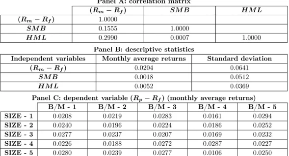
Table 3 – Dependent and independent variables
Panel A: correlation matrix
(Rm Rf) SM B HM L
(Rm Rf) 1.0000
SM B 0.1555 1.0000
HM L 0.2990 0.0007 1.0000
Panel B: descriptive statistics
Independent variables Monthly average returns Standard deviation
(Rm Rf) 0.0204 0.0641
SM B 0.0018 0.0512
HM L 0.0052 0.0369
Panel C: dependent variable (Rp Rf)(monthly average returns)
B/M - 1 B/M - 2 B/M - 3 B/M - 4 B/M - 5 SIZE - 1 0.0208 0.0219 0.0283 0.0161 0.0294 SIZE - 2 0.0240 0.0196 0.0224 0.0186 0.0252 SIZE - 3 0.0277 0.0237 0.0207 0.0169 0.0232 SIZE - 4 0.0226 0.0188 0.0272 0.0287 0.0227 SIZE - 5 0.0280 0.0239 0.0277 0.0106 0.0250
Panel A shows Pearson correlations between independent variables; Panel B shows mean and standard deviation of independent variables; Panel C shows monthly average returns of 25 portfolios sorted by size and book-to-market ratio (B/M)
3 portfolios sorted by B/M (L = low-B/M portfolio; M = medium-B/M portfolio; H = high-B/M portfolio); hence:
• SMB (small-minus-big): difference between the average return of three small portfolios and the average return of three big portfolios ⇣ (S/L)+(S/M )+(S/H) 3 (B/L)+(B/M )+(B/H) 3 ⌘ ;
• HML (high-minus-low): difference between the average return of two high-B/M portfolios and the average return of two low-B/M portfolios ⇣ (S/H)+(B/H) 2 (S/L)+(B/L) 2 ⌘ .
SMB and HML estimation procedure aims to remove the potential dependence be-tween size and B/M. The reliability of this technique is demonstrated by a very low correlation coefficient between SMB and HML (i.e., 0.0007, Table 3, panel A).
Three regression models may be summarized as follows:
Rpt Rf t= ↵p+ p(Rmt Rf t) + "pt, (3)
Rpt Rf t = ↵p+ spSM Bt+ gpHM Lt+ "pt, (4)
Rpt Rf t= ↵p+ p(Rmt Rf t) + spSM Bt+ gpHM Lt+ "pt, (5)
with p = 1, 2, . . . , 25 and t = 1, 2, . . . , 120. (Rpt Rf t), (Rmt Rf t), SMBt and
HM Ltare therefore vectors of 120 monthly returns. p, spand gpare regression
co-efficients expressing the sensitivity of portfolio risk premiums to time-series changes in market risk premium, size premium, and value premium, respectively.
Table 3 also shows average values of independent (panel B) and dependent (panel C) variables.
Table 4 – Monthly average returns and post-ranking beta for 25 SIZE-BETA port-folios
Panel A: monthly average returns (%)
All BETA - 1 BETA - 2 BETA - 3 BETA - 4 BETA - 5
All – 1.1541 1.1473 0.9984 0.8325 1.0859 SIZE - 1 1.3028 1.2895 1.3871 1.1981 1.1063 1.5329 SIZE - 2 1.0977 1.2875 1.3476 0.8545 0.9765 1.0223 SIZE - 3 1.0219 1.1934 1.3577 0.7453 0.6787 1.1345 SIZE - 4 0.8965 1.0134 0.8796 0.8563 0.8567 0.8765 SIZE - 5 0.8992 0.9865 0.7645 1.3376 0.5441 0.8634
Panel B: post-ranking beta
All BETA - 1 BETA - 2 BETA - 3 BETA - 4 BETA - 5
All – 0.8400 0.9800 0.7700 0.7700 0.8500 SIZE - 1 0.7700 0.7000 1.0200 0.6200 0.6400 0.8700 SIZE - 2 0.7500 0.7100 0.8900 0.5400 0.8700 0.7600 SIZE - 3 0.8000 0.9100 0.9800 0.7200 0.6500 0.7500 SIZE - 4 0.9100 0.8900 0.9900 1.0100 0.7100 0.9600 SIZE - 5 0.9700 1.0100 1.0100 0.9400 0.9800 0.9000
Panel A shows monthly average returns of 25 portfolios sorted by size and pre-ranking beta; Panel B shows post-ranking beta of 25 portfolios sorted by pre-post-ranking beta and size
4 Results
4.1 Descriptive analysis
Table 4 shows average monthly returns (Panel A) and portfolio post-ranking beta (Panel B) for each portfolio sorted by size and pre-ranking beta.
Table 4 allows us to outline a relationship between returns, size, and beta. Sort-ing stocks by size only (first column, Panel A), the smallest portfolio (SIZE - 1) earns a monthly return equal to 1.3028% compared to the largest portfolio that earns 0.8992% on average. In general, small stocks seem to produce higher aver-age returns than large stocks and this trend appears to hold also for each portfolio sorted by pre-ranking beta. However, when moving from large to small stocks, while returns go up, post-ranking beta does not (first column, Panel B) and this is not consistent with the SL model. Another relevant point is that a beta change (first row, Panel B) does not always go together with a same-type change of returns (first row, Panel A).
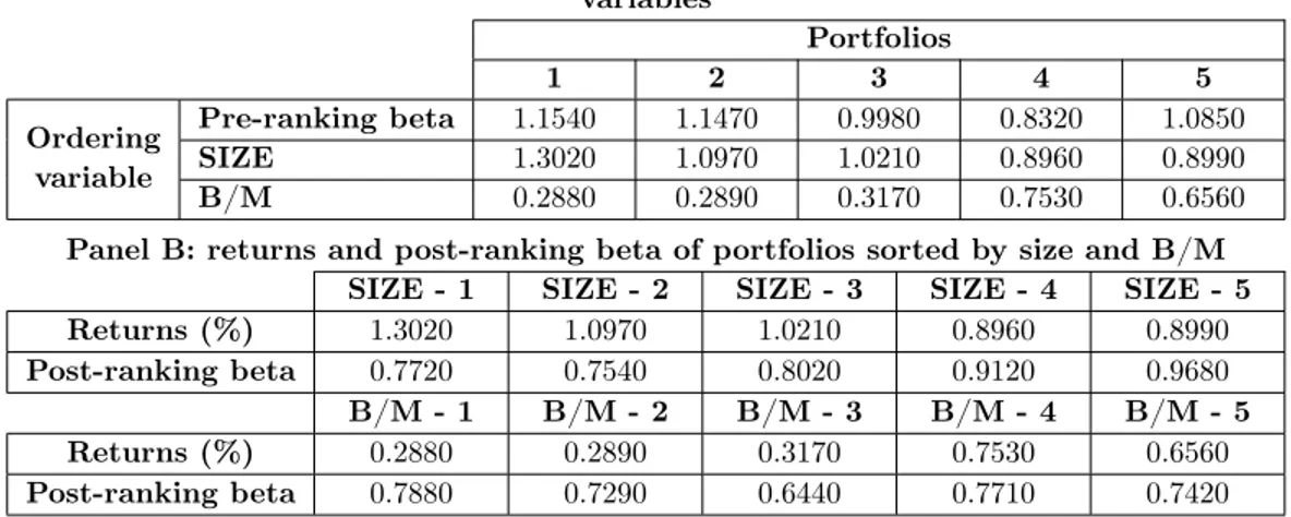
In June of each year, stocks are sorted in ascending order by each of the variables shown in Table 2 so as to form 5 portfolios whose monthly average returns are then estimated over a 120-month period (Table 5). Panel A of Table 5 shows these returns. Panel B of Table 5 reports monthly average returns and post-ranking beta of portfolios sorted by size and B/M.
The results show that high-B/M portfolios yield higher returns: Panel A shows that moving from portfolio 1 (B/M - 1) to portfolio 5 (B/M - 5), returns steadily increase from 0.288% to 0.656%. Size confirms the evidence already shown, that is, small firm portfolios earn greater returns than large firm portfolios.
Table 5 – Monthly average returns and post-ranking beta for 25 SIZE-BETA port-folios
Panel A: monthly average returns (%) of portfolios sorted by fundamental variables
Portfolios
1 2 3 4 5
Ordering Pre-ranking beta 1.1540 1.1470 0.9980 0.8320 1.0850
SIZE 1.3020 1.0970 1.0210 0.8960 0.8990
variable B/M 0.2880 0.2890 0.3170 0.7530 0.6560
Panel B: returns and post-ranking beta of portfolios sorted by size and B/M
SIZE - 1 SIZE - 2 SIZE - 3 SIZE - 4 SIZE - 5
Returns (%) 1.3020 1.0970 1.0210 0.8960 0.8990
Post-ranking beta 0.7720 0.7540 0.8020 0.9120 0.9680
B/M - 1 B/M - 2 B/M - 3 B/M - 4 B/M - 5
Returns (%) 0.2880 0.2890 0.3170 0.7530 0.6560
Post-ranking beta 0.7880 0.7290 0.6440 0.7710 0.7420
Panel A reports monthly average returns of portfolios sorted by each of the fundamental variables (pre-ranking beta, size, and B/M); Panel B reports returns and post-ranking beta of portfolios sorted by size and B/M
post-ranking beta. This means that higher returns earned by high-B/M portfolios do not seem to be explained by higher betas.
In summary, at this level of analysis, financial firms seem to behave in the same way as industrial firms in terms of risk factors: size and B/M appear to be linked to stock returns with small and high-B/M firms performing better than large and low-B/M firms. These relations do not seem to be explained by market beta and would support the implementation of a multifactor model of risk in which size premium and value premium are added to market risk premium.
4.2 Results of time-series regressions
Tables 6, 7, and 8 show results of time-series regressions run on each of three models, an SL model, a model with size premium and value premium alone, and a three-factor model respectively. Each row corresponds to the respective portfolio that the regression is performed on. Columns of the tables report, for each regression, regression coefficients ↵p, p, sp, gp, adjusted R2, and F -test significance level.
4.2.1 Regressions between portfolio risk premium and market risk premium Table 6 reports the following main results:
• Intercept is always statistically different from zero (except regression 18). This is not consistent with the SL model.
• Slope ( p) is always positive and significantly different from zero. Market risk
premium is therefore strongly linked to the risk premium of each portfolio according to the SL model. Market beta goes from a minimum of 0.4042 (portfolio 14) to a maximum of 1.4124 (portfolio 24). The bigger the firms in the portfolio, the larger the market beta seems to be, therefore showing that
Table 6 – Time-series regressions: returns and market risk premium ↵p p Adj. R2 sign(F ) 1 SIZE - 1 B/M - 1 ⇤0.0041 ⇤0.5895 0.3300 0.0000 2 B/M - 2 ⇤0.0146 ⇤0.4045 0.2359 0.0100 3 B/M - 3 ⇤0.0174 ⇤0.5307 0.3958 0.0120 4 B/M - 4 ⇤0.0041 ⇤0.5895 0.3380 0.0030 5 B/M - 5 ⇤0.0155 ⇤0.4351 0.3314 0.0040 6 SIZE - 2 B/M - 1 ⇤0.0101 ⇤0.4148 0.3054 0.0000 7 B/M - 2 ⇤0.0044 ⇤0.7417 0.3005 0.0000 8 B/M - 3 ⇤0.0118 ⇤0.5193 0.4210 0.0060 9 B/M - 4 ⇤0.0101 ⇤0.4148 0.3054 0.0080 10 B/M - 5 ⇤0.0150 ⇤0.5019 0.3992 0.0000 11 SIZE - 3 B/M - 1 ⇤0.0136 ⇤0.6902 0.4477 0.0020 12 B/M - 2 ⇤0.0034 ⇤0.9916 0.3959 0.0010 13 B/M - 3 ⇤0.0035 ⇤0.8449 0.3665 0.0000 14 B/M - 4 ⇤0.0086 ⇤0.4042 0.2284 0.0080 15 B/M - 5 ⇤0.0130 ⇤0.4980 0.2012 0.0000 16 SIZE - 4 B/M - 1 ⇤0.0005 ⇤1.0841 0.6684 0.0050 17 B/M - 2 ⇤0.0051 ⇤0.6708 0.5149 0.0110 18 B/M - 3 0.0096 ⇤0.8614 0.6247 0.0000 19 B/M - 4 ⇤0.0096 ⇤0.9319 0.4766 0.0000 20 B/M - 5 ⇤0.0057 ⇤0.9445 0.4239 0.0060 21 SIZE - 5 B/M - 1 ⇤0.0086 ⇤0.9525 0.5882 0.0000 22 B/M - 2 ⇤0.0023 ⇤1.0559 0.6907 0.0000 23 B/M - 3 ⇤0.0070 ⇤1.0148 0.5266 0.0000 24 B/M - 4 ⇤0.0149 ⇤1.4124 0.2887 0.0000 25 B/M - 5 ⇤0.0096 ⇤0.9251 0.3433 0.0000
⇤Statistically significant at 1% level
The table reports the results of the regression model in which returns of each portfolio are regressed on market risk premium: ↵pis the intercept, p is the slope, adj. R2measures the model goodness-of-fit, sign(F ) is the F -test level of significance
returns of large firms appear to be more sensitive to market risk. However, this result should be taken with caution because of the intervalling-effect bias in beta estimates. The sensitivity of a stock’s excess returns to the market excess returns is influenced by the length (e.g., daily, weekly, monthly, etc.) of the return interval used in estimating betas. Indeed, stock prices respond to new information more or less quickly depending on stock liquidity that, in turn, is affected by firm size. Small caps are less known, infrequently traded, and therefore adjust with delay, while large caps are better known, traded, and their price changes faster. As a consequence, for large firms, the smaller the length of the return interval, the higher the sensitivity of stock prices to market movements tends to be. Undersized return interval may therefore cause betas to be overestimated. While small caps show an opposite trend: betas tend to be overestimated when the return interval is oversized (e.g., Cohen et al., 1983, Jones and Yeoman, 2012, and Hong and Satchell, 2014).
• F -test always shows a high level of significance whereas the model goodness-of-fit is not always good: adjusted R2 is higher than 50% in 6 portfolios and
Table 7 – Time-series regressions: returns, SMB and HML ↵p sp gp Adj. R2 sign(F ) 1 SIZE - 1 B/M - 1 0.0147 -0.1985 ⇤⇤-0.2166 0.0239 0.0903 2 B/M - 2 0.0209 ⇤-0.1216 ⇤⇤-0.1919 0.0129 0.1876 3 B/M - 3 0.0271 ⇤-0.1396 -0.1792 0.0163 0.1416 4 B/M - 4 0.0147 -0.1985 ⇤⇤-0.2166 0.0239 0.0903 5 B/M - 5 0.0205 -0.1535 ⇤⇤0.0803 0.0140 0.1625 6 SIZE - 2 B/M - 1 0.0186 -0.2558 ⇤⇤0.0986 0.0658 0.0069 7 B/M - 2 0.0150 -0.3610 -0.7475 0.1349 0.0001 8 B/M - 3 0.0210 -0.3077 ⇤⇤-0.1689 0.0953 0.0011 9 B/M - 4 0.0186 -0.2558 0.0986 0.0658 0.0069 10 B/M - 5 0.0253 -0.2966 0.1218 0.0827 0.0024 11 SIZE - 3 B/M - 1 0.0225 -0.5203 -0.8046 0.3571 0.0000 12 B/M - 2 0.0164 -1.0308 -1.0353 0.0120 0.0000 13 B/M - 3 0.0178 -0.7231 ⇤⇤-0.3022 0.0760 0.0000 14 B/M - 4 0.0180 -0.3214 ⇤⇤0.3331 0.0330 0.0001 15 B/M - 5 0.0240 -0.3344 0.2690 0.0642 0.0077 16 SIZE - 4 B/M - 1 0.0159 -0.9951 -0.9453 0.3225 0.0000 17 B/M - 2 0.0171 -0.6003 -0.1163 0.3584 0.0000 18 B/M - 3 0.0243 -0.8910 -0.2538 0.0380 0.0000 19 B/M - 4 0.0256 -1.0426 -0.2250 0.0838 0.0000 20 B/M - 5 0.0205 -1.0674 0.0406 0.0586 0.0000 21 SIZE - 5 B/M - 1 0.0224 -1.2221 -0.6530 0.0098 0.0000 22 B/M - 2 0.0184 -1.2292 -0.6406 0.0799 0.0000 23 B/M - 3 0.0227 -1.1586 -0.5741 0.0898 0.0000 24 B/M - 4 0.0049 -1.9485 -0.3430 0.0753 0.0000 25 B/M - 5 0.0256 -1.3210 0.6055 0.0085 0.0000
⇤ Statistically significant at 5% level
⇤⇤Statistically significant at 10% level
The table reports the results of the regression model in which returns of each portfolio are regressed on SMB and HML factors: ↵pis the constant, spis the SMB coefficient, gpis the HML coefficient, adj. R2measures the model goodness-of-fit, sign(F ) is the F -test level of significance
in 3 of them exceeds 60%. In the remainder of them, it is almost always lower than 30% and shows the need to find additional risk factors other than market risk.
• Larger R2 (i.e., greater than 50%) are found in portfolios with large firms
(SIZE-4 and SIZE-5). This shows that portfolio return variability explained by market risk premium is bigger in large-sized firms.
4.2.2 Regressions between portfolio risk premium, SMB, and HML
SMB and HML factors on their own cannot describe portfolio excess returns well (Table 7). F -test is almost always significant (except 5 portfolios), but R2 is very
poor: it exceeds 30% in only 3 portfolios and the others show R2 always lower than
10% (except portfolio 7).
SMB regression coefficients are negative and decrease the larger the firm size. This means that spis greater in absolute value in portfolios of large firms. However,
SMB coefficients are almost never statistically significant (only portfolios 2 and 3 show statistically significant coefficients at the 5% level). Portfolio excess returns are not therefore sensitive to size premium.
Moving from low-B/M portfolios to high-B/M portfolios, HML coefficients gp
tend to grow according to Fama and French (1993), but in 17 out of 25 portfolios, they are not statistically significant. As a consequence, we cannot draw reliable conclusions about the effect of the value premium on the portfolio excess return. Combining size- and value-based portfolios does not seem to be useful to construct an efficient portfolio.
4.2.3 Regressions between portfolio risk premium, market risk premium, SMB, and HML
Table 8 shows the results of the third model in which portfolio risk premium is regressed on market risk premium, SMB, and HML simultaneously. The explana-tory power of the model significantly improves and this is not due to collinearity between independent variables (Table 3, Panel A). We can draw the following main conclusions:
• p is positive and statistically significant (except for portfolios 2, 9, and 10).
This confirms that market risk premium is a risk factor that should be included in the model.
• spis now statistically significant in almost all portfolios and seems to be positive
for small portfolios (SIZE - 1 and SIZE - 2) and negative for larger portfolios. This result is consistent with the presence of a small size effect in the financial industry too. Investors seem to require an additional risk premium to be willing to hold small stocks (see Section 2 for the relevant literature on non-financial firms). A plausible explanation is that small banks do not benefit from govern-ment assistance should distress occur. Large banks are protected by implicit government guarantees linked to their systemic role.
• gp is not statistically significant in only 5 portfolios and, within a size class,
high-B/M portfolios show higher regression coefficients than low-B/M portfo-lios. High-B/M firms seem to be more sensitive to the value premium and therefore pay a higher risk premium to investors that hold these stocks. • Adjusted R2are significantly higher than those found in the previous two
mod-els. They are below 50% in only 7 portfolios, range between 50% and 70% in an additional 12 portfolios, and get to about 80% in the remaining 6 portfolios. Higher values concentrate on portfolios of large firms. The three-factor model appears to have good power in explaining portfolio excess return variability in the financial sector.
• The constant of the model ↵p is never statistically different from zero,
demon-strating that time-series variations of returns are systematically explained by three risk premiums.
Table 8 – Time-series regressions: returns, market risk premium, SMB and HML ↵p p sp gp Adj. R2 sign(F ) 1 SIZE - 1 B/M - 1 0.0020 ⇤0.7700 0.3358 ⇤0.1830 0.4779 0.0000 2 B/M - 2 0.0131 0.5325 ⇤0.2494 0.0644 0.5627 0.0000 3 B/M - 3 0.0151 ⇤0.7265 0.3646 ⇤0.1979 0.5725 0.0000 4 B/M - 4 0.0020 ⇤0.7700 ⇤0.3358 ⇤0.1830 0.4779 0.0000 5 B/M - 5 0.0101 ⇤0.6315 ⇤0.2849 ⇤0.4082 0.5449 0.0000 6 SIZE - 2 B/M - 1 0.0099 ⇤0.5279 ⇤0.1105 ⇤0.3726 0.5695 0.0000 7 B/M - 2 0.0026 ⇤0.7514 ⇤0.1604 -0.3574 0.4219 0.0000 8 B/M - 3 0.0113 ⇤0.5868 0.0995 ⇤0.1357 0.5238 0.0000 9 B/M - 4 0.0099 0.5279 ⇤0.1105 ⇤0.3726 0.4695 0.0000 10 B/M - 5 0.0146 0.6489 ⇤0.1537 ⇤0.4587 0.5928 0.0000 11 SIZE - 3 B/M - 1 0.0138 ⇤0.5326 ⇤-0.1507 ⇤-0.5282 0.6180 0.0000 12 B/M - 2 0.0067 ⇤0.5909 ⇤-0.6208 ⇤-0.7286 0.5950 0.0000 13 B/M - 3 0.0049 ⇤0.7381 -0.1796 ⇤0.1043 0.4664 0.0000 14 B/M - 4 0.0093 ⇤0.5290 ⇤0.0457 ⇤0.6077 0.4742 0.0000 15 B/M - 5 0.0132 ⇤0.6566 0.1213 ⇤0.6098 0.3797 0.0000 16 SIZE - 4 B/M - 1 0.0028 ⇤0.7963 ⇤-0.4425 ⇤-0.5319 0.8424 0.0000 17 B/M - 2 0.0066 ⇤0.6378 ⇤-0.1577 ⇤0.2147 0.6421 0.0000 18 B/M - 3 0.0127 ⇤0.7007 ⇤-0.4047 0.1099 0.7901 0.0000 19 B/M - 4 0.0138 ⇤0.7142 ⇤-0.5470 0.1452 0.6532 0.0000 20 B/M - 5 0.0098 ⇤0.7458 ⇤-0.5540 ⇤0.3998 0.6092 0.0000 21 SIZE - 5 B/M - 1 0.0143 ⇤0.4944 ⇤-0.8690 ⇤-0.3963 0.8059 0.0000 22 B/M - 2 0.0074 ⇤0.6641 ⇤-0.7684 ⇤-0.2958 0.8467 0.0000 23 B/M - 3 0.0117 ⇤0.6670 ⇤-0.6957 ⇤-0.2279 0.7271 0.0000 24 B/M - 4 0.0058 ⇤0.7284 ⇤-1.4409 ⇤0.0076 0.5176 0.0000 25 B/M - 5 0.0160 ⇤0.6991 ⇤-0.8530 0.9241 0.7387 0.0000
⇤Statistically significant at 5% level
The table reports the results of the regression model in which returns of each portfolio are regressed on market risk premium, SMB and HML factors: ↵p is the constant, p is the market risk premium coefficient, sp is the SMB coefficient, gp is the HML coefficient, adj. R2 measures the model goodness-of-fit, sign(F ) is the F -test level of significance
5 Conclusions
In this study we test the Fama-French three-factor model employed in the estimation of financial stock returns in Europe. The analysis shows the following main results: • Market risk premium significantly affects stock returns in every model and its presence is required if the model is to have sufficient explanatory power. When it is used alone as in the SL model, it works better in portfolios of large firms. • Size and B/M are demonstrated to be cross-sectionally linked to stock returns: small firms and high-B/M firms show higher returns that market beta cannot explain.
• Size premium and value premium help explain time-series changes of returns only when they are used with market risk premium. Regression coefficients sp
and gp are almost always significantly different from zero in the three-factor
• Investors require an extra return for small and high-B/M stocks that seem to be more sensitive to changes in the risk premium related to size and B/M factors. In light of the above results, financial stocks traded in the European stock ex-changes yield returns that reward risks linked to small size and high B/M in addition to market risk. This means that the need to price financial stocks may benefit from a multifactor model of risk in which size and B/M appear to be sources of risk as in non-financial industries. We do not mean that size and B/M necessarily proxy for the same risk sources as for non-financial firms, but rather that being small and with a high B/M induces investors to ask for an additional risk premium in the financial sector too.
All of this has relevant implications for financial system and banking authorities. In the last decades, banks have diversified their revenue streams by significantly in-creasing proceeds generated by non-traditional, high-income activities such as invest-ment banking. This, among other things, was the result of increased competition, deregulation, and financial market integration (e.g., Bessler and Kurmann, 2014). Moreover, the level of opaqueness of bank balance sheets has increased because of the expansion of complex and hard-to-value financial instruments and the rise of the to-distribute model that took the place of the traditional, originate-to-hold model. Finally, bank leverage has increased significantly over the past 100 years (e.g., DeAngelo and Stulz, 2013) especially in large financial institutions.
These factors contributed to change bank risk exposure, made prudential rules on capital requirements outdated, and induced supervisors to introduce new frameworks for regulating capital adequacy, stress testing, and market liquidity risk. Banking authorities therefore require instruments to control for factors reflecting a large number of risks, from the traditional ones to the emerging ones. In this context, the use of market measures in the regulatory process, such as the book-to-market ratio and the market leverage, may help supervisory institutions to assess bank risk exposure better.
While value premium seems to be relevant in estimating risk premium of finan-cial and non-finanfinan-cial firms, the existence of a size premium is more ambiguous. In the financial sector, one can presume that large banks are more diversified and therefore less risky than smaller banks. However, the too big to fail policy may encourage irresponsible risk taking. The empirical evidence is mixed: some stud-ies (e.g., Demsetz and Strahan, 1997) demonstrate that large and diversified banks work with less capital and undertake riskier projects, while some other (e.g., Konishi and Yasuda, 2004) finds a negative relationship between size and bank risk taking. More recent studies on size anomalies in US bank stock returns (Gandhi and Lustig, 2015) confirm that shareholders of large banks bear less risk and earn significantly lower risk-adjusted returns than those of small banks even though the former are significantly more leveraged than the latter. This evidence may be a result of gov-ernment protections that support large banks. We confirm this result and show that investors seem to require higher returns to smaller banks but this point is still controversial (e.g., Goyal, 2014).
References
Allen, M. T., Madura, J., and Wiant, K. J. (1995). “Commercial Bank Exposure and Sensitivity to the Real Estate Market”, Journal of Real Estate Research, 10:129–140. Al-Mwalla, M., and Karasneh, M. (2011). “Fama & French Three Factor Model: Evidence from Emerging Market”, European Journal of Economics, Finance and Administrative Sciences, 41:132–140.
Arshanapalli, B. G., Coggin, T. D., and Doukas J. (1998). “Multifactor Asset Pricing Analysis of International Value Investment Strategies”, The Journal of Portfolio Management, 24:10–23.
Baek, S., and Bilson, J. F. O. (2014). “Size and Value Risk in Financial Firms”, Journal of Banking and Finance, in press.
Banz, R. (1981). “The Relationship Between Return and Market Value of Common Stocks”, Journal of Financial Economics, 9:3–18.
Barber, B. M., and Lyon, J. D. (1997). “Firm Size, Book-to-Market Ratio, and Security Returns: A Holdout Sample of Financial Firms”, The Journal of Finance, 52:875–883.
Beaver, W., Kettler, P., and Scholes, M. (1970). “The Association Between Mar-ket Determined and Accounting Determined Risk Measures”, Accounting Review, 45:654–682.
Berk, J. (1995). “A Critique of Size Related Anomalies”, Review of Financial Studies, 8:275–286.
Bessler, W., and Booth, G. (1994). “Interest Rate Sensitivity of Bank Stock Re-turns in a Universal Banking System”, Journal of International Financial Markets, Institutions, and Money, 3:117–136.
Bessler, W., and Kurmann, P. (2014). “Bank Risk Factors and Changing Risk Ex-posures: Capital Market Evidence Before and During the Financial Crisis”, Journal of Financial Stability, 13:151–166.
Bessler, W., and Murtagh, J. P. (2004). “Risk Characteristics of Banks and Non-Banks: An International Comparison”, in Geberl, S., Kaufmann, H. R., Menichetti, M. J., and Wiesner, D. F. (Eds.), Aktuelle Entwicklungen im Finanzdienstleistungs-bereich (pp. 65–78). Berlin: Springer-Verlag.
Black, F. (1972). “Capital Market Equilibrium with Restricted Borrowing”, Journal of Business, 45:444–455.
Black, F., Jensen, M. C., and Scholes, M. (1972). “The Capital Asset Pricing Model: Some Empirical Tests”. In Jensen, M. C. (ed.), Studies in the Theory of Capital Markets (pp. 79–121). New York: Praeger Publishers, Inc.
Brennan, M. J. (1970). “Taxes, Market Valuation and Corporate Financial Policy”, National Tax Journal, 23:417–427.
Chamberlain, S., Howe, J. S., and Popper, H. (1997). “The Exchange Rate Exposure of US and Japanese Banking Institutions”, Journal of Banking and Finance, 21:871– 892.
Chan, K. C., and Chen, N. (1988). “An Unconditional Asset Pricing Test and the Role of Firm Size as an Instrumental Variable for Risk”, Journal of Finance, 43:309– 325.
Chan, K. C., Karceski, J., and Lakonishok, J. (2000). “New Paradigm or Same Old Hype in Equity Investing?”, Financial Analysts Journal, 56:23–36.
Choi, J. J., Elyasiani, E. (1997). “Derivative Exposure and the Interest Rate and Exchange Rate Risks of US Banks”, Journal of Financial Services Research, 12: 267–286.
Choi, J. J., Elyasiani, E., and Kopecky, K. (1992). “The Sensitivity of Bank Stock Returns to Market, Interest and Exchange Rate Risks”, Journal of Banking and Finance, 16:983–1004.
Cohen, K. J., and Hawawini, G. A., Maier, S. F., Schwartz, R. A., and Whitcomb, D. K. (1983). “Estimating and Adjusting for the Intervalling-Effect Bias in Beta”, Management Science, 29:135–148.
Daniel, K., and Titman, S. (1997). “Evidence on the Characteristics of Cross Sec-tional Variation in Stock Returns”, The Journal of Finance, 52:1–33.
Davis, J. L., Fama, E. F., and French, K. R. (2000). “Characteristics, Covariances, and Average Returns: 1929 to 1997”, The Journal of Finance, 55:389–406.
DeAngelo, H., and Stulz, R. M. (2013). Why High Leverage is Optimal for Banks, NBER Working Paper No. 19139.
Demsetz, R. S., and Strahan, P. E. (1997). “Diversification, Size, and Risk at Bank Holding Companies”, Journal of Money, Credit and Banking, 29:300–313.
Dewenter, K. L., and Hess, A. C. (1998). “An International Comparison of Banks’ Equity Returns”, Journal of Money, Credit and Banking, 30:472–492.
Dimson, E., and Marsh, P. (1999). “Murphy’s Law and Market Anomalies”, Journal of Portfolio Management, 25:53–69.
Eraslan, V. (2013). “Fama and French Three-factor Model: Evidence from Istanbul Stock Exchange”, Business and Economics Research Journal, 4:11–22.
Fama, E. F., and French, K. R. (1992). “The Cross-Section of Expected Stock Re-turns”, The Journal of Finance, 47:427–465.
Fama, E. F., and French, K. R. (1993). “Common Risk Factors in the Returns on Stocks and Bonds”, Journal of Financial Economics, 33:3–56.
Fama, E. F., and French, K. R. (2012). “Size, Value, and Momentum in International Stock Returns”, Journal of Financial Economics, 105:457–472.
Fama, E. F., and MacBeth, J. (1973). “Risk, Return and Equilibrium: Empirical Tests”, The Journal of Political Economy, 81:607–636.
Flannery, M. J., and James, C. M. (1984). “The Effect of Interest Rate Changes on the Common Stock Returns of Financial Institutions”, The Journal of Finance, 39:1141–1153.
Foye, J., Mramor, D., and Pahor, M. (2013). “A Respecified Fama French Three-Factor Model for the New European Union Member States”, Journal of International Financial Management & Accounting, 24:3–25.
Gandhi, P., and Lustig, H. (2015). “Size Anomalies in US Bank Stock Returns”, The Journal of Finance, 70:733–768.
Gibbons, M. R. (1982). “Multivariate Tests of Financial Models: A New Approach”, Journal of Financial Economics, 10:3–27.
Giliberto, M. (1985). “Interest Rate Sensitivity in the Common Stocks of Finan-cial Intermediaries: A Methodological Note”, Journal of FinanFinan-cial and Quantitative Analysis, 20:123–126.
Gounopoulos, D., Molyneux, P., Staikouras, S. K., Wilson, J. O. S., and Zhao, G. (2013). “Exchange Rate Risk and the Equity Performance of Financial Intermedi-aries”, International Review of Financial Analysis, 29:271–282.
Goyal, A. (2014). No Size Anomalies in U.S. Bank Stock Returns, available at SSRN: http://ssrn.com/abstract=2410542.
Griffin, J. M. (2002). “Are the Fama and French Factors Global or Country Specific?”, Review of Financial Studies, 15:783–803.
Hess, A. C., and Laisathit, K. (1997). “A Market-Based Risk Classification of Fi-nancial Institutions”, Journal of FiFi-nancial Services Research, 12:133-158.
Hong, K. H. J., and Satchell, S. (2014). “The Sensitivity of Beta to the Time Horizon when Log Prices Follow an Ornstein-Uhlenbeck Process”, The European Journal of Finance, 20:264–290.
Horowitz, J. L., Loughran, T., and Savin, N. E. (1999). “The Disappearing Size Effect”, Research in Economics, 54:83–100.
Horowitz, J. L., Loughran, T., and Savin, N. E. (2000). “Three Analyses of the Firm Size Premium”, Journal of Empirical Finance, 7:143–153.
Jones, S. L., and Yeoman, J. C. (2012). “Bias in Estimating the Systematic Risk of Extreme Performers: Implications for Financial Analysis, the Leverage Effect, and Long-Run Reversals”, Journal of Corporate Finance, 18:1–21.
Kane, E. J., and Unal, H. (1988). “Change in Market Assessments of Deposit-Institution Riskiness”, Journal of Financial Services Research, 1:207–229.
Konishi, M., and Yasuda, Y. (2004). “Factors Affecting Bank Risk Taking: Evidence from Japan”, Journal of Banking and Finance, 28:215–232.
Kothari, S. P., Shanken, J., and Sloan, R. (1995). “Another Look at the Cross-Section of Expected Stock Returns”, The Journal of Finance, 50:185–224.
Lindenberg, E. (1979). “Capital Market Equilibrium with Price Affecting Institu-tional Investors”, in Elton, E. J., and Gruber, M. J. (Eds.), Portfolio Theory 25 Years After. Amsterdam: North-Holland Publishing Company.
Lintner, J. (1965). “The Valuation of Risk Assets and the Selection of Risky Invest-ments in Stock Portfolios and Capital Budgets”, Review of Economics and Statistics, 47:13–37.
Lynge, M. J., and Zumwalt, J. K. (1980). “An Empirical Study of the Interest Rate Sensitivity of Commercial Bank Returns: A Multi-Index Approach”, Journal of Financial and Quantitative Analysis, 15:731–742.
Manjunatha, T., and Mallikarjunappa, T. (2011). “Does Three-Factor Model Explain Asset Pricing in Indian Capital Market?”, Decision, 38:119–140.
Martins, A. M., Serra, A. P., and Martins, F. V. (2012). Real Estate Market Risk in Bank Stock Returns: Evidence for 15 European Countries, CEF.UP Working Paper No. 1203, University of Porto.
Mayers, D. (1972), “Nonmarketable Assets and Capital Market Equilibrium under Uncertainty”, in Jensen, M. C., (Ed.), Studies in the Theory of Capital Markets. New York: Praeger Publishers, Inc.
Mayshar, J. (1981). “Transaction Costs and the Pricing of Assets”, The Journal of Finance, 36:583–597.
Mei, J., and Saunders, A. (1995). “Bank Risk and Real Estate: An Asset Pricing Perspective”, Journal of Real Estate Finance and Economics, 10:199–224.
Miller, M., and Scholes, M. (1972). “Rates of Return in Relation to Risk: A Re-Examination of Some Recent Findings”, in Jensen, M. C. (Ed.), Studies in the Theory of Capital Markets. New York: Praeger Publishers, Inc.
Modigliani, F., and Miller, M. (1958). “The Cost of Capital, Corporation Finance and the Theory of Investment”, The American Economic Review, 48:261–297. Modigliani, F., and Miller, M. (1963). “Corporate Income Taxes and the Cost of Capital: A Correction, The American Economic Review, 53:433–443.
Moerman, G. A. (2005). How Domestic is the Fama and French Three-Factor Model? An Application to the Euro Area, ERIM Report Series Reference No. ERS-2005-035-F&A.
Mossin, J. (1966). “Equilibrium in A Capital Asset Market”, Econometrica, 34:768– 783.
Oertmann, P., Rendu, C., and Zimmermann, H. (2000). “Interest Rate Risk of Eu-ropean Financial Corporations”, EuEu-ropean Financial Management, 6:459–478. Roll, R. (1977). “A Critique of the Asset Pricing Theory’s Tests: Part I: On Past and Potential Testability of the Theory”, Journal of Financial Economics, 4:129–176. Ross, S. (1976). “The Arbitrage Theory of Capital Asset Pricing”, Journal of Eco-nomic Theory, 13:341–360.
Schuermann, T., and Stiroh, K. J. (2006). Visible and Hidden Risk Factors for Banks, Staff Report No. 252, Federal Reserve Bank of New York.
Sehgal, S., and Balakrishnan, A. (2013). “Robustness of Fama-French Three Factor Model: Further Evidence for Indian Stock Market”, Vision: The Journal of Business Perspective, 17:119–127.
Sharma, R., and Mehta, K. (2013). “Fama and French: Three Factor Model”, Journal of Indian Management, 1:90–105.
Sharpe, W. F. (1964). “Capital Asset Prices: A Theory of Market Equilibrium under Conditions of Risk”, The Journal of Finance, 19:425–442.
Stambaugh, R. F. (1982). “On the Exclusion of Assets from Tests of the Two-Parameter Model: A Sensitivity Analysis”, Journal of Financial Economics, 10:237– 268.
Taneja, Y. P. (2010). “Revisiting Fama French Three-Factor Model in Indian Stock Market”, The Journal of Business Perspective, 14:267–274.
Treynor, J. (1962). Toward a Theory of the Market Value of Risky Assets, unpub-lished manuscript.
Viale, A. M., Kolari, J. W., and Fraser, D. R. (2009). “Common Risk Factors in Bank Stocks”, Journal of Banking and Finance, 33:464–472.
• n.46: Farina, F. Development theory and poverty. A review
• n.45: Croci Angelini E., Farina F., Valentini E. Contagion across Eurozone’s sovereign spreads and the Core-Periphery divide
• n.44: Cutrini E., Galeazzi G. Contagion in the Euro crisis: capital flows and trade linkages
• n.43: Carlin W., Schaffer M., Seabright P. Soviet power plus electrification: what is the long-run legacy of communism?
• n.42: Clementi F., Giammatteo M. The labour market and the distribution of income: an empirical analysis for Italy
• n.41: Cutrini E., Galeazzi G. Can emerging economies decouple from the US business cycle?
• n.40: Cutrini E., Micucci G., Montanaro P. I distretti tradizionali di fronte alla globalizzazione: il caso dell’industria calzaturiera marchigiana
• n.39: Bade F.-J., Bode E., Cutrini E. Spatial fragmentation of industries by functions
• n.38: Gentilucci E., Herrera R. Un’analisi critica dei lavori recenti del main-stream sugli effetti economici delle spese militari
• n.37: Stefani G., Cavicchi A. Consumer evaluation of a typical Italian salami: an experimental auction approach
• n.36: Valentini E. Giving Voice to Employees and Spreading Information within the Firm: the Manner Matters
• n.35: Cutrini E., Valentini E. What drives economic specialization in Italian Regions?
• n.34: Spigarelli F., Goldstein A., Manzetti L. Italian economic diplomacy at work: catching up the BRICs
• n.33: Cutrini E., Spigarelli F. Italian FDI integration with Southeast Europe: country and firm-level evidence
• n.32: Davino C., Romano R. Sensitivity Analysis of Composite Indicators through Mixed Model Anova
• n.31: Rocchi B., Cavicchi A., Baldeschi M. Consumers’ attitude towards farm-ers’ markets: an explorative analysis in Tuscany
• n.30: Trinchera L., Russolillo G. On the use of Structural Equation Models and PLS Path Modeling to build composite indicators
• n.29: Tavoletti E. The internationalization process of Italian fashion firms: the governance role of the founding team
• n.28: Croci Angelini E. Globalization and public administration: a complex relationship
• n.27: Tavoletti E. Matching higher education and labour market in the knowl-edge economy: the much needed reform of university governance in Italy
• n.25: Ciaschini M., Pretaroli R., Severini F., Socci C. Environmental tax reform and double dividend evidence
• n.24: Atkinson A. B. Poverty and the EU: the New Decade
• n.23: Cutrini E. Moving Eastwards while Remaining Embedded: the Case of the Marche Footwear District, Italy
• n.22: Valentini E. On the Substitutability between Equal Opportunities and Income Redistribution
• n.21: Ciaschini M., Pretaroli R., Socci C. La produzione di servizi sanitari e la variazione dellÕoutput nei principali paesi UE
• n.20: Cassiani M., Spigarelli F. Gli hedge fund: caratteristiche, impatto sui mercati e ruolo nelle crisi Þnanziarie
• n.19: Cavicchi A. Regolamentazione e gestione del rischio nel settore agroal-imentare. Alcune riflessiioni sull’approccio economico al Principio di Pre-cauzione
• n.18: Spalletti S. The History of Manpower Forecasting in Modelling Labour Market
• n.17: Boffa F., Pingali V. MIncreasing Market Interconnection: an analysis of the Italian Electricity Spot Market
• n.16: Scoppola M. Tariffication of Tariff Rate Quotas under oligopolistic com-petition: the case of the EU import regimes for bananas
• n.15: Croci Angelini E., Michelangeli A. Measuring Well-Being differences across EU Countries. A Multidimensional Analysis of Income, Housing, Health, and Education
• n.14: Fidanza B. Quale comparable per la valutazione tramite multipli delle imprese Italiane?
• n.13: Pera A. Changing Views of Competition and EC Antitrust Law • n.12: Spigarelli F. Nuovi investitori globali: le imprese cinesi in Italia
• n.11: Ciaschini M., Pretaroli R., Socci C. A convenient multi sectoral policy control for ICT in the USA economy
• n.10: Tavoletti E., te Velde R. Cutting Porter’s last diamond: competitive and comparative (dis)advantages in the Dutch flower industry. Which lessons for Italian SMEs?
• n.9: Tavoletti E. The local and regional economic role of universities: the case of the University of Cardiff
• n.8: Croci Angelini E. Resisting Globalization: Voting Power Indices and the National Interest in the EU Decision-making
• n.7: Minervini F., Piacentino D. Spectrum Management and Regulation: To-wards a Full-Fledged Market for Spectrum Bands?
• n.5: Ciaschini M., Fiorillo F., Pretaroli R., Severini F., Socci C., Valentini E. Politiche per l’industria: ridurre o abolire l’Irap?
• n.4: Scoppola M. Economies of scale and endogenous market structures in international grain trade
• n.3: De Grauwe P. What have we learnt about monetary integration since the Maastricht Treaty?
• n.2: Ciaschini M., Pretaroli R., Socci C. A convenient policy control through the Macro Multiplier Approach
• n.1: Cave M. The Development of Telecommunications in Europe: Regulation and Economic Effects