Alma Mater Studiorum
· University of Bologna
School of Science
Department of Physics and Astronomy Master Degree in Physics
On the Kolmogorov property of a class of
infinite measure hyperbolic dynamical
systems
Supervisor:
Prof. Marco Lenci
Submitted by:
Giovanni Canestrari
2
Sono tornato l`a dove non ero mai stato. Nulla, da come non fu, `e mutato.
Sul tavolo (sull’incerato a quadretti) ammezzato ho ritrovato il bicchiere
mai riempito. Tutto `e ancora rimasto quale
mai l’avevo lasciato.
Sommario
Le mappe lisce con singolarit`a descrivono importanti fenomeni fisici come l’urto tra sfere rigide tra loro e/o con le pareti di un contenitore. Le domande sulle propriet`a ergodiche di questi sistemi (che possono essere mappati in sistemi di tipo biliardo) furono sollevate per primo da Boltzmann nel diciannovesimo secolo e pongono i fondamenti della Meccanica Statistica. I sistemi di tipo biliardo descrivono anche i moti di↵usivi di elettroni che urtano contro nuclei di carica positiva (gas di Lorentz) e in questo caso la misura fisica preservata dalla dinamica pu`o essere considerata a tutti gli e↵etti come infinita. E’ dunque di grande importanza studiare le propriet`a ergodiche di mappe che preservano una misura infinita. Lo scopo di questa tesi `e di presentare un risultato originale sulle mappe liscie con singolarit`a che preservano una misura infinita. Tale risultato dimostra l’atomicit`a della -algebra di coda (e dunque forti propriet`a stocastiche) in presenza di un comportamento totalmente conservativo.
Abstract
Smooth maps with singularities describe important physical phenomena such as the col-lisions of rigid spheres among them and/or with the walls of a container. Questions about the ergodic properties of these models (which can be mapped into billiard mod-els) were first raised by Boltzmann in the nineteenth century and lie at the foundation of Statistical Mechanics. Billiard models also describe the di↵usive motion of electrons bouncing o↵ positive nuclei (Lorentz gas models) and in this situation the physical mea-sure can be considered infinite. It is therefore of great importance to study the ergodic properties of maps when the measure they preserves is infinite. The aim of this thesis is to present an original result on smooth maps with singularities which preserve an infinite measure. Such result establishes the atomicity of the tail -algebra (and hence strong chaotic properties) in the presence of a totally conservative behavior.
Contents
1 Introduction 8
1.1 Lorentz gas . . . 9
1.2 Hard balls . . . 10
2 Some notions of infinite ergodic theory 14 2.1 Recurrence and conservativity . . . 15
2.2 Conditions for conservativity . . . 20
3 Measurable partitions, -algebras and disintegration 24 3.1 Abstract Measure Theory . . . 24
3.2 Lebesgue spaces . . . 26
3.2.1 Isomorphism and conjugacy . . . 26
3.2.2 Defining Lebesgue spaces . . . 28
3.3 Partitions and -algebras . . . 33
3.4 Measurable partitions . . . 34
3.5 Disintegration . . . 37
4 Billiards 40 4.1 Billiard tables . . . 44
4.2 Billiard map . . . 46
4.2.1 Phase space for the flow . . . 47
4.2.2 Collision map . . . 47
4.2.3 Coordinates for the map and its singularities . . . 49
4.2.4 Invariant measure of the map . . . 50
4.2.5 Involution . . . 50
4.3 Lyapunov exponents and hyperbolicity . . . 51
4.3.1 Lyapunov exponents for the map . . . 55
4.3.2 Proving hyperbolicity: cone techniques . . . 58
4.3.3 Cones and geometrical optics . . . 61
4.4 LSUM: the role of singularities . . . 64
4.4.1 Hyperbolicity . . . 65
Contents 6
4.4.2 Singularities . . . 68
4.4.3 Stable and unstable manifolds . . . 72
4.4.4 Size of unstable manifolds . . . 76
5 A Direct Proof of the K-Property for the Baker’s Map 80 5.1 Kolmogorov automorphisms . . . 80
5.2 Definition of the map . . . 80
5.3 Some basic facts about -algebras and partitions . . . 81
5.4 The Proof . . . 82
6 A Structure Theorem for Infinite Measure Maps with Singularities 86 6.1 Exactness, K-mixing and partitions . . . 86
6.2 Setup and result . . . 88
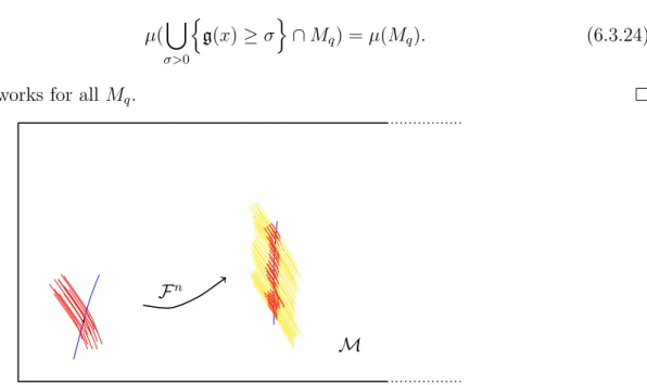
6.3 Proof of the Structure Theorem . . . 92
6.4 Distortion . . . 101
6.4.1 Assumptions for distortion . . . 101
6.4.2 Relations between assumptions . . . 104
6.4.3 Proving distortion estimates . . . 105
6.5 Distortion of the return map to a global cross section . . . 107
6.6 Existence and measurability of a partition into homogeneous LSUMs . . 112
6.6.1 Existence . . . 112
6.6.2 Measurability . . . 114
6.7 Applications . . . 117
6.7.1 Lorentz Gases and Tubes . . . 117
Chapter 1
Introduction
In this thesis we present an original result that states that certain billiard-like systems (smooth, hyperbolic maps with singularities) enjoy strong chaotic properties, even when they have infinite measure. In particular, we prove that these dynamical systems have an atomic tail -algebra with respect to their partition into stable manifolds. This result has been proved for finite measure billiard-like systems by Pesin [Pes1,Pes2], but his methods seem unable to be easily carried over to the infinite measure case because of the use of entropy theory therein. Billiards are mathematical models for many physical systems where one or more particles collide with the walls of a container and/or with each other. The dynamical properties of such models are determined by the shape of the walls of the container, and may vary from completely regular (integrable) to fully chaotic. The most intriguing, though least elementary, are chaotic billiards. They include the classical models of hard balls studied by L. Boltzmann in the nineteenth century, the Lorentz gas introduced to describe electricity in 1905, as well as modern dispersing billiard tables due to Ya. Sinai. The mathematical theory of chaotic billiards was born in 1970 when Ya. Sinai published his seminal paper [S], and is now 50 years old. But during these years it has grown and developed at a remarkable speed and has become a well established and flourishing area within the modern theory of dynamical systems and statistical mechanics. The aim of this introduction is to explain why a physicist or a mathematician may be interested in the dynamics of billiards. We have already mentioned two applications, namely the Lorentz gas [Lo] and the hard ball systems. To explain a little better what these systems have in common with billiards we shortly define billiard dynamics. We anticipate here some definitions that will be studied in greater detail later.
Definition 1.0.1. LetD ⇢ R2 be a domain with smooth or piece-wise smooth boundary.
A billiard system corresponds to a free motion of a point particle insideD with specular reflections o↵ the boundary @D.
The definition of billiard dynamics mirrors almost perfectly the physics of the billiard
1.1 Lorentz gas 9
D
B A
Figure 1.
game the reader is certainly familiar with. The main di↵erences being two: the billiard ball is point-like and moves without friction for an infinite time (except when it hits a corner and ends up in the hole) and the billiard table is not necessarily rectangular-shaped but can assume a great variety of shapes. A billiard table may look, for example, like this:
The thick black line, which defines the domain D ⇢ R2, represent the wall of the
con-tainer. When the trajectory of the ball (dotted line) meets them, it bounces o↵ following the classical rule ‘angle of incidence is equal to the angle of reflection’. The two gray disks A and B are called scatterers. Usually, they are not included in D by definition, but behave exactly as the wall: the ball bounces o↵ them with the usual rule. When they are present the system resembles more a flipper than a billiard. We will see later that the configuration space of two hard-balls colliding on a torus maps exactly into a billiard system with a point-like particle bouncing elastically o↵ the walls.
1.1
Lorentz gas
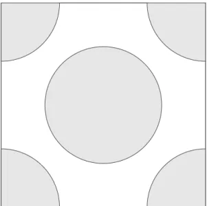
One can also consider D ⇢ T2 instead as D ⇢ R2. In this case D = T2 r [O
i, where
Oi are the scatterers. Convex billiards defined on the torus are called Sinai billiards1,
in honor of Ya. Sinai who first carried a detailed study of them [S]. Upon lifting2 the
system to R2, the motion of the billiard ball in this infinite flipper exactly defines the
dynamics of a periodic Lorentz gas (PLG), in which an electron bounces o↵ the positive
1For a more precise definition of Sinai billiard see the next sections.
2Leaving aside the precise definition of ‘lifting’, it simply means that we ”tessellate” the planeR2with
infinite identical copies of our fundamental domainT2 (and of course along with it we copy everything that stays inside the fundamental domain).
1.2 Hard balls 10
nuclei.
lift to R2
Figure 2.
Note that the Lorentz gas (which is the lifted version inR2) is similar to the billiard on
the torus. A remarkable di↵erence between the two models is that the ‘unlifted’ version has finite measure while the lifted one infinite. Nonetheless, one tries to infer statistical properties of the Lorentz gas studying the ‘smaller’ system on the torus, which is a canonical example of chaotic billiard. Indeed, the original part of this thesis goes in this direction. In this program, a key property that has to be satisfied by the lifted system with infinite measure is that of conservativity almost everywhere. Roughly speaking, every electron that starts its motion from one of the scatterer has to retrace itself and pass close to where it started infinitely many times in the future. This property is also called recurrence and expresses the concept that history repeats itself. For periodic Lorentz gas the problem of recurrence has ba✏ed mathematicians for decades, and was answer in the affirmative only in the last few years, by Schmidt [Sch] and Conze [Co] independently. A further progress has been achieved by Lenci [L3, L4] who proved the recurrence for a certain class of aperiodic Lorentz gases. Therefore, it is of great interest to better understand the implications of recurrence, in terms of the statistical properties of the dynamics when it comes along with others properties of the map.
1.2
Hard balls
Here we describe a mechanical system of two hard disks that reduces to a dispersing billiard. This mechanical model is actually a prototype of all dispersing billiard tables and is the model that motivated Sinai to introduce dispersing billiards after he studied the motion of hard disks and hard balls in the 1960s.
1.2 Hard balls 11
torus T2 without obstacles or walls of any kind. The disks move freely with constant
velocities and collide with each other elastically, as described below. Let the disks collide and denote their velocity vectors before the collisions by u and v . Let L denote the common tangent line to the disks at the moment of collision. For every vector v denote by v? and v|| its components perpendicular and parallel to the line L, respectively. We
call v|| the tangential component of v and v? the normal component of v.
According to the law of elastic collision, the postcollisional velocity vectors of the disks are
u+ = u|| + v? and v+= v|| + u?. (1.2.1)
In other words, the velocity vectors keep their tangential components but exchange their normal components. Observe that this rule implies the preservation of the total kinetic energy
||u+||2+||v+||2 =||u ||2+||v ||2
and the total momentum
u++ v+= u + v
(recall that the disks have unit mass). The conservation of the total momentum implies that the center of mass (xc, yc) moves on the torus with a constant velocity vector. This is
a simple periodic or quasi periodic motion, and we eliminate it from the picture assuming that the total momentum is zero; i.e. u + v = 0 at all the times.
Now the center of mass is at rest. More precisely, let 0 x, y 1 denote rectangular coordinates onT2 and (x
1, y1) and (x2, y2) the centers of our disks. Choose the coordinate
systems so that, initially, the center of mass
xc =
1
2(x1+ x2) and yc = 1
2(y1+ y2) coincides with the center of the torus (1
2, 1
2); equivalently,
x1+ x2 = 1 and y1+ y2 = 1. (1.2.2)
Clearly, since the total momentum is zero, the position of the center of mass remains constant and Equation (1.2.2) will hold at all times. The coordinates x and y are cyclic, so they can occasionally increase or decrease by one; therefore, when x1 increases by
one, for example, then x2 must decrease by one. Next, the disks collide with each other
whenever the distance between their centers is 2r, i.e. whenever
(x1 x2+ p)2+ (y1 y2+ q)2 = (2r)2
for some p = 0,±1 and q = 0, ±1. Due to (1.2.2), this is equivalent to ⇣ x1 1 p 2 ⌘2 +⇣y1 1 q 2 ⌘2 = r2. (1.2.3)
1.2 Hard balls 12
Simple substitution of the possible values of p, q 2 {0, ±1} shows that Equation (1.2.3) specifies four circles of radius r with centers at (0, 0), (0,1
2), ( 1 2, 0) and ( 1 2, 1 2). Let Oi
denotes the circles (1.2.3). We now examine the transformation of the velocity vectors u and v at collisions. Since u + v = 0, we obviously have u|| = v|| and u? = v? in
the notation of (1.2.1); therefore
u+= u|| u? and v+ = v|| v?.
In other words, each velocity vector simply gets reflected o↵ the common tangent line L of the colliding disks. Observe that L is parallel to the tangent line to the circle Oi on
which the point (x1, y1) lies at the moment of collision. Also note that ||u|| = ||v|| = p
2 2
remain constant in time.
Therefore, the center (x1, y1) of the first disk moves onT2 with a constant velocity vector
until it hits one of the circlesOi. Then its velocity gets reflected across the tangent line
to that circle at the point of hit, and so on. This is exactly a billiard trajectory3 on the
table T2r [O i.
3To be precise, the point (x
1, y1) moves at a constant, but not unit, speed. One can rescale the time
Chapter 2
Some notions of infinite ergodic
theory
In this chapter we deal with the property of conservativity. While for finite measure measure preserving transformations conservativity is just a corollary (it is the content of a theorem by Poincar´e), in the case of infinite measure conservativity is not assured and it gains a central role in the development of the theory. Here, the aim is just to define this property and characterize it a little bit but we will always stay quite near the surface of the infinite ergodic theory. A great part of this summary owes to the first chapter of the book of Aaronson [A], which is a very detailed introduction to the subject. Let us start by describing the very basics of ergodic theory and by stating the Poincar´e theorem for the finite measure case.
A measure space is the triple (X, A, µ) where X is a set, A is a -algebra on X and µ is a measure on (X, A). A measure space (X, A, µ) is said probability space if µ(X) = 1. Often, it is required that the measure space is nice enough by asking it to be a standard measure space.
Definition 2.0.1. A Polish space is a complete, separable metric space. Let X be a Polish space. The collection of Borel sets B(X) is the -algebra of subsets of X generated by the collection of open sets.
Definition 2.0.2. A standard measurable space (or standard Borel space) (X, B) is a Polish space X equipped with its Borel sets.
Definition 2.0.3. A standard measure space is a measure space (X, B, m) where (X, B) is a standard measurable space.
Standard measure spaces can be regarded as the bridge from topological notions and measure-theoretic ones, in that they assign positive measure to the open sets.
Definition 2.0.4. Let (X, B, m) and (X0, B0, m0) be measure spaces, and let A 2 B, A0 2 B0. The map T : A ! A0 is measurable if T 1C 2 B 8C 2 B0. The measurable
2.1 Recurrence and conservativity 15
map T : A ! A0 is called invertible on B 2 B \ A if T is 1-1 on B, T B 2 B0, and
T 1 : T B ! B is measurable.
Standard ergodic theory studies measure preserving maps in probability spaces. An extension of the notion of preservation of measure is non-singularity.
Definition 2.0.5. The measurable map T : A ! A0 is called (two-sided) non-singular
if for C 2 B0 \ A0, one has
m(T 1C) = 0() m(C) = 0. and measure preserving if m(T 1C) = m(C) for C 2 B0\ A0.
2.1
Recurrence and conservativity
One property that is enjoyed by all measure-preserving transformations in probability spaces is recurrence:
Theorem 2.1.1. (Poincar´e’s Recurrence Theorem) Let T : X ! X be a measure pre-serving transformation of a probability space (X, B, m). Let E 2 B with m(E) > 0. Then almost all points of E return infinitely often to E under positive iterations by T (i.e., there exists F ✓ E with m(F ) = m(E) such that for each x 2 F there is an infinite sequence n1 < n2 < n3 < ... of natural numbers with Tni(x)2 F for each i).
Proof. For N 0 let EN = S1n=NT nE. Then T1N =0EN is the set of all points of
X which enter E infinitely often under positive iterations of T . Hence the set F = E \ T1N =0EN consists of all points of E that enter E infinitely often under positive
iterations by T . If x2 F then there is a sequence n1 < n2 < n3 < ... of natural numbers
with Tni(x)2 E for all i. For each i we have also Tni(x)2 F because Tnj ni(Tnix)2 E
for all j. It remains to show m(F ) = m(E). Since T 1E
N = EN +1 we have m(EN) = m(EN +1) and hence m(E0) = m(EN) for all
N . Since E0 ◆ E1 ◆ E2 ◆ ... we have m(T1N =0EN) = m(E0). Therefore m(F ) =
m(E\ E0) = m(E) since E ✓ E0.
Remark 2.1.2. 1. In the proof the measure-preserving property of T was used only in the weaker form of incompressibility (i.e., if B 2 B and T 1B ✓ B then m(B) =
m(T 1B)). Therefore Theorem 2.1.1 is true for incompressible transformations.
2. Theorem 2.1.1 is false if a measure space of infinite measure is used. An example is given by the map T (x) = x + 1 defined onZ with the measure on Z which gives each integer unit measure. For this example if E denotes the set{0} then the set EN all have infinite measure but T1N =0EN is empty.
2.1 Recurrence and conservativity 16
That property, that holds automatically for measure-preserving transformations on probability spaces, is called recurrence.
Definition 2.1.3. We say that a measure-preserving map T on a (possibly infinite) measure space (X, B, m) is recurrent if for every positive measure set A 2 B almost every x2 A has the property that Tnix2 A for an infinite sequence of natural numbers
n1 < n2 < n3 < ... .
An equivalent definition is the one in [A]:
Definition 2.1.4. A non singular transformation T on (X, B, m) is recurrent if
lim inf
n!1 |h T
n h| = 0 a.e. 8h : X ! R measurable.
These two definitions are equivalent. Indeed, the second implies the first simply by choosing h = 1Afor any A2 B of positive measure (we write A 2 B+); the fact that the
second definition implies the first will be clear after the prosecution of our discussion. We begin by studying the extremely non-recurrent behavior exhibited by wondering sets. Let T be a non-singular transformation of the standard measure space (X, B, m). Definition 2.1.5. A set W ⇢ X is called a wondering set (for T ) if the sets {T nW}1
n=0
are disjoint. Let W = W(T ) denote the collection of measurable wondering sets. Note that T 1W(T ) ✓ W(T ).
The next result dichotomize, and localize the recurrent behavior of a non-singular transformation. Denote by B+ the sets in B with positive measure.
Theorem 2.1.6. (Halmos’ recurrence theorem) Suppose that A2 B, m(A) > 0, then m(A\ W ) = 0 8W 2 W () 1 X n=1 1B Tn =1 on B 8B 2 B+\ A. Proof. ()).
Assume that B 2 B and m(B \ W ) = 0 8W 2 W. Let B =
1
[
n=1
T nB. Clearly T 1B ✓ B . We claim that W
B := Br B is a wondering set for T . To see
this, we note that WB ✓ T nBc ✓ T nWBc 8n 1. whence T nWB \ T mWB = ;
8n 6= m. Since WB 2 W, WB ⇢ B, we have (by assumption) that m(WB) = 0. Thus
2.1 Recurrence and conservativity 17 By the non-singularity of T , 8n 1, m(T nW B) = 0 and so T nB ✓ T nB mod m, whence ( mod m), B ✓ B = T 1B = T 2B = ... = 1 \ k=1 1 [ n=k T nB ={ 1 X n=1 1B Tn=1}. (().
Conversely, if9W 2 W so that m(W \ A) > 0, then clearly
1
X
n=1
1B Tn= 0 on B := W \ A 2 B+.
Now we would like to define maximal sets in which there is wondering and recurrent behavior. To do so we have to face the problem that a union of arbitrary many measurable sets (such as the wondering sets) is not necessarily measurable. It turns out that in the case of wondering sets this is not a real problem because W(T ) is what is called an hereditary collection.
Definition 2.1.7. Let (X, B, m) be a measure space. A collection H ✓ B is called hereditary if
C 2 H, B ⇢ C, B 2 B =) B 2 H. The hereditary collections have measurable unions.
Definition 2.1.8. A set U 2 B is said to cover the hereditary collection H if A ✓ U mod m 8A 2 H.
A hereditary collection H✓ B is said to saturate U 2 B if 8B 2 B, B ✓ U, m(B) > 0, 9C 2 H, m(C) > 0, C ✓ B.
The set U 2 B is called measurable union of the hereditary collection H ✓ B if it both covers and is saturated by H.
A good property of a measurable union is that there is no more than one for each hereditary collection. To see this, let U and U0 2 B be measurable unions of the
hereditary collection H and suppose that m(U r U0) > 0. Then, (since H saturates U ) there exists C 2 H, m(C) > 0, C ✓ U r U0, whence (since U0 covers H) C ✓ U0 mod m
contradicting m(C) > 0. This shows that U ✓ U0 mod m and by symmetry U = U0
2.1 Recurrence and conservativity 18
Theorem 2.1.9. (Exhaustion lemma) Let (X, B, m) be a probability space and let H✓ B be hereditary, then 9 A1, A2, ... 2 H disjoint such that U(H) = S1n=1An is a measurable
union of H. Proof. Let
✏1 := sup{m(A) : A 2 H},
choose A1 2 H such that m(A1) ✏21, and let
✏2 := sup{m(A) : A 2 H, A \ A1 =;},
choose A2 2 H such that A2 \ A1 = ; and m(A2) ✏22. Continuing the process, we
obtain a sequence of disjoint{An}1n=1 ✓ H and decreasing {✏k}k such that
✏n := sup{m(A) : A 2 H, A \ Ak =; 8k < n}, m(An)
✏n
2.
Clearly,P1n=1✏n 2P1n=1m(An) 2, whence ✏n! 1. We claim that U :=S1n=1An =
X is a measurable union of H. Evidently H saturates U . To see that U covers H assume otherwise, then9A 2 H, m(A) > 0 such that A \ An=; 8n 1 whence m(A) ✏n ! 0
contradicting m(A) > 0.
One can extend the previous result to the case when (X, B, m) is -finite. In that case X = S1j=1Bj for some measurable finite-measure sets Bj and one can apply Theorem
2.1.9 to H\ Bj, and then make a union over all Bj.
Remark 2.1.10. The Exhaustion Lemma tells us two things: that measurable unions exists and that they can be expressed by countable unions. In this notes we actually need only the first part but also the second is important.
We are ready to define the conservative and dissipative part of a non singular trans-formation.
Definition 2.1.11. The dissipative part of the non singular transformation T is D(T ) := U (W(T )), i.e. the measurable union of the collection of wondering sets for T . The non-singular transformation T is called (totally) dissipative if D(T ) = X mod m.
Since T 1W(T ) ✓ W(T ), we have that T 1D✓ D mod m.
Definition 2.1.12. The set C(T ) := Xr D(T ) is called the conservative part of T . The non-singular transformation T is called (totally) conservative if C(T ) = X mod m.
Definition 2.1.13. The Hopf decomposition of T is the partition of X {C(T ), D(T )}. Let us see a first corollary of the Halmos’ Recurrence Theorem.
2.1 Recurrence and conservativity 19
Corollary 2.1.14. If T is a non-singular transformation, then
C(Tn) = C(T ) mod m, 8n 1.
Proof. We prove that D(Tn) = D(T ). Since W(T ) ✓ W(Tn) it is clear that D(T ) ✓
D(Tn). On the other hand, if W 2 W(Tn)
+, then T jW 2 W(Tn)+ and 1 X k=1 1W Tk = n X j=1 1 X k=0 1T jW Tnk n a.e. on W.
By Halmos’ Recurrence Theorem, there exists W0 2 W(T )
+\W . Thus m(W rD(T )) = 0
8W 2 W(Tn), whence
D(Tn)✓ D(T ) mod m.
Now, we have defined both conservative and recurrent transformations. In the next theorem and subsequent corollary we prove that these two definitions are actually equiv-alent. Let B(z, ✏) be the ball at z with radius ✏.
Theorem 2.1.15. (Poincar´e’s Recurrence Theorem) Suppose that T : X ! X is a conservative, non-singular transformation of (X, B, m). If (Z, d) is a separable metric space, and f : X ! Z is a measurable map, then
lim inf
n!1 d(f (x), f (T
nx)) = 0 for a.e. x2 X.
Proof. Let Z1 ={z 2 Z : m(f 1(B(z, ✏))) > 0 8✏ > 0}, a closed subset of Z. Since (Z, d)
is separable,9{B(xn, ✏n)}n✓ Z1c such that Z1c =
S
nB(xn, ✏n) whence m(Xrf 1(Z1)) =
0. We show that lim infn!1d(f (x), f (Tnx)) = 0 a.e. for x 2 X
1 := f 1(Z1). By the
Halmos’ Recurrence Theorem, for z2 Z1 and ✏ > 0, 1 X k=1 1f 1(B(z,✏)) Tk =1 a.e. on f 1(B(z, ✏)), whence lim inf n!1 d(f, f T n) < 2✏ a.e. on f 1B(z, ✏),8z 2 Z 1, ✏ > 0.
Fix ✏ > 0. By separability, there exists a sequence {zn : zn 2 Z1, n 2 N+} such that
Z1 =S1n=1B(zn, ✏), whence
lim inf
n!1 d(f, f T
n) < 2✏ a.e. on f 1Z
2.2 Conditions for conservativity 20
We take inspiration form the preceding theorem to define yet another kind of recur-rence.
Definition 2.1.16. If (Z, d) is a separable metric space, we call a non singular trans-formation T on (X, B, m) Z-recurrent if lim infn!1d(f, f Tn) = 0 a.e. whenever
f : X ! Z is measurable.
Theorem 2.1.17. Let T be a non singular transformation of (X, B, m). The following are equivalent.
1. T is Z-recurrent for some separable metric space (Z, d) containing at least two points.
2. T is Z-recurrent for every separable metric space (Z, d). 3. T is conservative.
Proof. By Theorem 2.1.15, (3) ) (2) and clearly (2) ) (1). We are left to prove that (1)) (3). Let A 2 B+ and take z1, z2 2 Z such that d(z1, z2) c for some fixed c > 0.
Then define fA: X ! Z by
fA(x) =
(
z1, if x2 A
z2, if x2 Ac
Clearly fA is measurable. Consider the ball B(z1, ✏) centered at z1 with radius ✏. If we
choose ✏ < c, we have lim inf n d(fA T n(x), f A(x)) = 0 a.e. on f 1(B(z1, ✏)) =) 1 X k=1 1A Tk(x) =1.
Therefore, the thesis follows from Halmos’ Recurrence Theorem.
Corollary 2.1.18. Every recurrent transformation in the sense of Definition 2.1.4 is recurrent in the sense of Definition 2.1.3.
Proof. Indeed the Definition 2.1.4 of recurrence it is just R-recurrence in the language of Definition 2.1.16. By Theorem 2.1.17 this implies conservativity of T and therefore by Halmos’ Recurrence theorem Definition 2.1.3 is satisfied.
2.2
Conditions for conservativity
If there exists a finite, T -invariant measure q ⌧ m, then clearly there can be no won-dering sets with positive q-measure (the disjoint union of their pre-images would build
2.2 Conditions for conservativity 21
up an infinite q-measure). Therefore, q(D) = 0 and {dmdq > 0} ✓ C mod m. In par-ticular, any probability preserving transformation is conservative. A measure-preserving transformation of a -finite, infinite measure space may not be conservative. For exam-ple, x 7! x + 1 is a measure preserving transformation of R equipped with Borel sets and Lebesgue measure, which is totally dissipative. The following propositions help to establish conservativity of measure preserving transformations of -finite measure spaces. Proposition 2.2.1. Suppose that T is a measure preserving transformation of the -finite measure space (X, B, m).
1. If f 2 L1(m), f 0, then ( 1 X k=1 f Tk =1 ) ✓ C(T ) mod m. 2. If f 2 L1(m), f > 0 a.e., then ( 1 X k=1 f Tk =1 ) = C(T ) mod m.
Proof. We first show (1). Let f 2 L1(m)
+, it is sufficient to show thatP1k=1f Tk <1
a.e. on any W 2 W. To see this let W 2 W and n 1, then Z W n X k=0 f Tkdm = n X k=0 Z X 1Wf Tn kdm = n X k=0 Z X 1W Tkf Tndm = = Z X n X k=0 1W Tk f Tndm Z X f Tndm = Z X f dm. Therefore, Z W n X k=0 f Tkdm Z X f dm <1 and n X k=0 f Tkdm <1 a.e. on W.
We now prove (2). In view of (1), for f 2 L1(m), f > 0 a.e, it suffices to show that
C(T )✓ {
1
X
k=1
2.2 Conditions for conservativity 22
Indeed, for all A2 B+, A ✓ C(T ), there exists B ✓ A and ✏ > 0 such that f ✏1B on
B, whence 1 X k=1 f Tk ✏ 1 X k=1 1B Tk =1, a.e. on B,
by Halmos’ Recurrence Theorem.
The last result we present is the following theorem.
Theorem 2.2.2. Suppose that T is a measure preserving transformation of the -finite measure space (X, B, m). If there exists A2 B, m(A) < 1 such that
X = 1 [ n=0 T nA mod m, then T is conservative.
Proof. Note that
X = T kX =
1
[
n=k
T nA mod m,
for all k 1. Therefore, P1n=11ATn = 1 almost everywhere. The thesis then follows
Chapter 3
Measurable partitions, -algebras
and disintegration
The aim of this chapter is to present Rokhlin theorem on the disintegration of measures. Our main references are [W], [CK] and Appendix B of [B]. The original proof of the Rokhlin theorem is presented in [R1] and other useful and related materials (with greater emphasis on entropy theory) is in [R2].
3.1
Abstract Measure Theory
We report here some concepts of abstract measure theory as presented in the very clear exposition of [CK]. There are three ‘lenses’ trough which we can view measure theory; we may think of it in terms of points, sets or functions. Suppose we have a triple (X, B, m) comprising a measure space, a -algebra and a measure. Then we may focus on the set X (and concern ourselves with points), or on the -algebra B (and concern ourselves with sets), or on the space L2(X, B, m) (and concern ourselves with functions). All
three point of view play an important role in dynamics, and various definitions and results can be given in terms of any of the three. We will see later that the last two are completely equivalent in the greatest generality but the first requires certain additional, albeit natural, assumptions explained in the next section. To be even more specific, it will be of particular interest to us the correspondence between partitions of the space X, sub- -algebras of B and subspaces of L2(X, B, m).
First let us consider the set of all partitions of X. This is a partially ordered set, with ordering given by refinement; given two partitions ⇠, ⌘, we say that ⇠ is a refinement of ⌘, written ⇠ ⌘, if and only if every C 2 ⇠ is contained in some D 2 ⌘. In this case, we also say that ⌘ is a coarsening of ⇠. The finest partition is the partition into points, denoted ✏, while the coarsest is the trivial partition {X}, denoted ⌫. As on any partially ordered set, we have a notion of join (or product) and meet (or intersection),
3.1 Abstract Measure Theory 25
corresponding to least upper bound and greater lower bound, respectively. Given two partitions ⇠ and ⌘, their join is
⇠_ ⌘ := {C \ D|C 2 ⇠, D 2 ⌘}. (3.1.1) This is the coarsest partition which refines both ⇠ and ⌘, and is also sometimes referred to as the joint partition. For a finite or countable family {⇠n}, the join ⇠ = Wn⇠n is
a partition whose elements are (nonempty) intersections \nCn, where Cn 2 ⇠n for all
n. One can also consider the case in which {⇠↵}↵ is not countable and the join is still
defined (as the coarsest partition which is finer than each ⇠↵), but it has not that simple
characterization anymore. The meet of ⇠ and ⌘ is the finest partition which coarsen both ⇠ and ⌘, and is denoted ⇠^ ⌘. In general there is no simple analogue to (3.1.1) for ⇠ ^ ⌘ (even in the countable case!). Indeed, given a finite or countable family of measurable partitions {⇠m}, one may attempt to construct their meet Vm⇠m as follows. For any
x, y 2 X we put x ⇠ y if there exists a finite sequence A1, ..., An 2 [m⇠m such that
x2 A1 and y2 An and Ai\ Ai+1 6= ; for all 1 i n 1 (of course for each i the sets
Ai and Ai+1 must be elements of di↵erent partitions here, because their intersection in
non-empty). Then ⇠ will be an equivalent relation on X and its classes naturally define a partition of X; we call it ˜^m⇠m. The partition ˜^m⇠m corresponds, ‘logically’, to the
meets ^m⇠m, and in many cases ^m⇠m = ˜^m⇠m mod 0. But in some cases ˜^m⇠m may
be quite di↵erent from ^m⇠m (in fact, ˜^m⇠m may not even be measurable), so it is not
safe to use it in lieu of ^m⇠m.
Example 1. Let X = [0, 1] and µ the Lebesgue measure on X. Let ⇠1 ={[0, 0.5], (0, 5, 1]}
and ⇠2 ={{0, 1}, {x}}x2Xr{0,1} (⇠2 is a partition of X into the set{0, 1} and all one-point
subsets of X r {0, 1}). As one can verify1
⇠1^ ⇠2 = ⇠1 but ⇠1^⇠˜ 2 = ⌫.
Anyway we mention that this problem can be fixed when we are in a Lebesgue space. In that case one can prove that there exists a full measure set D ⇢ X such that if we denote by ⇠D the partition ⇠ restricted to the set D (i.e. ⇠D ={C \ D|C 2 ⇠} it holds
˜
^m⇠m,D =^m⇠m,D,
whenever ˜^m⇠m,D is measurable (the interested reader may look at the Appendix B of
[CM]).
Given a partition ⇠, we may consider the collection of all measurable subsets A⇢ X, which are unions of elements of ⇠; this collection forms a sub- -algebra of B which we
1Note that the equality for partitions below is to be intended mod 0, a concept that we will clarify
3.2 Lebesgue spaces 26
will denote by F(⇠). We will see later that this correspondence is far from injective; for example, certain partitions whose elements are countable sets are associated with the trivial -algebra.
Similarly, we can consider the collection of all square integrable functions which are constant on elements of ⇠; the collection of all equivalence classes of such functions forms the subspace L2(X, F(⇠), µ) ⇢ L2(X, B, µ).
Example 2. Let X = [0, 1]⇥ [0, 1] be the unit square with Lebesgue measure Leb2 and
B the Borel -algebra. Let ⇠ = n{x} ⇥ [0, 1]|x 2 [0, 1]o be the partition into vertical lines; then F(⇠) is the sub- -algebra consisting of all sets of the form E⇥ [0, 1], where E ✓ [0, 1] is Borel, and L2(X, F(⇠), Leb
2) is the space of all square-integrable functions
which depend only on the x-coordinate. The latter is canonically isomorphic to the space of square-integrable functions on the unit interval.
The map ⇠ ! F(⇠) is a morphisms of partially ordered sets; it is natural to ask whether this morphism in injective (and hence invertible) on a certain class of partitions. First, however, we turn to the question of classifying measure spaces and hence the associated class of -algebras and partitions, since the end result turns out to be relatively simple. It turns out that such a classification will also be crucial for the problem of correspondence between partition and sub- -algebras.
3.2
Lebesgue spaces
It is somewhat serendipitous that although one may consider many di↵erent measure spaces (X, B, µ), which on the face of it are quite di↵erent from each other, all of the examples in which we will be interested actually fall into a relatively simple classification. To elucidate this statement, let us consider the two fundamental examples of measure spaces. The simplest sort of measure space is an atomic space, in which X is a finite or countable space. At the other hand of the spectrum stand the non-atomic spaces, in which every positive measure set can be decomposed into two subsets of smaller positive measure. The easiest example of such a space is the interval [0, 1] with Lebesgue measure. In fact, up to isomorphism and setting aside examples which are for our purpose pathological, this is the only example of such a space.
3.2.1
Isomorphism and conjugacy
What does it mean for measure space to be isomorphic? The most immediate (and essentially correct) idea is to require existence of a bijection between the spaces which carries measurable sets into measurable sets both ways and preserves the measure. Ob-viously such a bijection must be in accordance with one of the fundamental principles of measure theory: disregarding null-measure sets.
3.2 Lebesgue spaces 27
Definition 3.2.1. (Measure space isomorphism) The probability spaces (X1, B1, m1)
and (X2, B2, m2) are said to be isomorphic if there exists M1 2 B1 and M2 2 B2
with m1(M1) = 1 and m2(M2) = 1 and an invertible measure-preserving transformation
: M1 ! M2. (The space Mi is assumed to be equipped with the -algebra Mi \ Bi =
{Mi\ B|B 2 Bi} and the restriction of the measure mi to this -algebra.)
This definition cares about points because we ask to be an isomorphisms. If we decide to focus on sets, the most natural way of define an ‘isomorphism’ disregarding sets of zero measure is trough what is called -algebras isomorphisms or conjugacy. This requires that we define first measure algebras.
Definition 3.2.2. Let (X, B, m) be a probability space. Define an equivalence relation on B by saying that A and B are equivalent (A⇠ B) i↵ m(A4B) = 0. Let ˜B denote the collection of equivalence classes. Then ˜B is a Boolean -algebra under the operation of complementation, union and intersection inherited from B. The measure m induces a measure ˜m on ˜B by ˜m( ˜B) = m(B). (Here ˜B is the equivalence class to which B belongs). The pair ( ˜B, ˜m) is called a measure algebra.
Definition 3.2.3. Let (X1, B1, m1) and (X2, B2, m2) be probability spaces with
mea-sure algebras ( ˜B1, ˜m1) and ( ˜B2, ˜m2). The measure algebra are isomorphic if there is a
bijection : ˜B2 ! ˜B1 which preserves complements, countable unions and intersections
and satisfies ˜m1( ˜B) = ˜m2( ˜B) for any ˜B 2 ˜B2. The probability spaces are said to be
conjugate if their measure algebras are isomorphic.
Conjugacy of measure spaces is weaker than isomorphism because if (X1, B1, m1)
and (X2, B2, m2) are isomorphic as in Definition 3.2.1 then they are conjugate via :
˜
B2 ! ˜B1 defined by ( ˜B) := ( 1(M2 \ B))⇠. On the other hand, it is easy to give
examples of conjugate measure spaces which are not isomorphic. Let (X1, B1, m1) be a
space of one point and (X2, B2, m2) be a space of two points and B2 ={;, X2}. The two
spaces are conjugate but they are not isomorphic because a set of zero measure cannot be omitted from X2 so that the remaining set is mapped bijectively with X1. The main
reason this example works is that B2 does not separate the points of X2. What is nice
about Lebesgue spaces is that they are designed in such a way that this never happens and everything works so that isomorphism and conjugacy are equivalent. So, actually, in these spaces there is in principle no conceptual gap between a point-description and a set-description of measure theory. What is even nicer about Lebesgue spaces is that they are isomorphic (with the stronger Definition 3.2.1 and so also with the weaker one 3.2.3), with the measure space ([0, 1], L, Leb1), where L are the Borel subsets2 of [0, 1]
and Leb1 is the Lebesgue measure. So, to sum up:
1. In Lebesgue spaces isomorphism and conjugacy are equivalent;
2Actually the Lebesgue subsets, i.e. the completion of the Borel -algebra, because we assume always
3.2 Lebesgue spaces 28
2. Lebesgue spaces are isomorphic to ([0, 1], L, Leb1).
In some books such as [W] Lebesgue spaces are defined precisely by saying that they are isomorphic to ([0, 1], L, Leb1) (with a possible addition of countably many atoms).
We follow another route: in the next section we will present a couple of theorems that basically say that if the measure space has some good properties then it is more and more similar to ([0, 1], L, Leb1). We then put in the defintion of Lebesgue space exactly
the conditions one needs to make a generic measure space isomorphic to ([0, 1], L, Leb1).
In doing so, we will find out that these conditions are precisely the ones that make isomorphisms equivalent to conjugacy.
3.2.2
Defining Lebesgue spaces
Let us introduce a metric dµ on the measure algebra ( ˜B, ˜m) by the formula
dµ( ˜A, ˜B) = µ(A4B),
where A and B are some representative elements of the equivalence classes ˜A and ˜B, respectively. ( ˜B, dµ) is a metric space.
Definition 3.2.4. We say that the -algebra B is separable if ( ˜B, dµ) is separable
as a metric space. That is, B is separable i↵ there exists a countable collection of equivalence classes of set{ ˜An}n2Nwhich is dense in ˜B with the metric dµ. If one consider
representative elements A of each ˜A then dµ is not anymore a metric but becomes a
pseudo-metric (two di↵erent sets can have zero distance). In this case B is separable i↵ there exists a countable collection of sets {An}n2N which is dense in B with the
pseudo-metric dµ.
Definition 3.2.5. The completion of B is the -algebra generated by B together with all subsets of null sets (one can prove that this collection of sets is indeed a -algebra, see e.g. [Sc]). We say that two -algebra are equivalent mod 0 if they have the same completion.
From now on we will consider only complete -algebras, unless otherwise specified, and when we will say that two -algebras are equal we may forget to say that they are equal mod 0.
Recall that ifA ✓ B is any collection of sets, then (A), the -algebra generated by A, is the smallest -algebra that contains A.
Proposition 3.2.6. Let (X, B, m) be a probability space. If B is equivalent mod zero to a -algebra generated by a countable collection of sets, then B is separable.
3.2 Lebesgue spaces 29
Proof. Let A = {An}n2N be the countable collection of sets that generates B. Let
A⇤ = {A⇤
k}k2N be the set of all finite unions of elements of A, which is countable. Let
us denote ¯A⇤ the closure of A⇤ un the d
µ metric. Clearly ¯A⇤ contains A. It can also
be shown that ¯A⇤ is closed under intersection and countable union. This shows that ¯A⇤
contains B and henceA⇤ is dense in B.
Corollary 3.2.7. Let X be a separable metric space, B its the Borel -algebra and µ a probability measure. Then B is separable as a -algebra.
Theorem 3.2.8. Let (X, B, m) be a probability space. Let also ( ˜B, ˜m) be a separable measure algebra (complete) with no atoms. Then ( ˜B, ˜m) is isomorphic to the -algebra of Lebesgue sets of the unit interval. In other words, the probability space (X, B, m) is conjugated to ([0, 1], L, Leb1).
Proof. (Sketch) Given a countable collection of sets {An} 2 B, write A0n := An and
A1
n := X r An, and let ⇠n =
Wn
i=1{A0n, A1n}. This is an increasing sequence of partitions
of X, and because B is separable, we may take the sets An to be such that ˆB :=
S
n 1B(⇠n) is dense in B. Moreover ⇠n has 2n elements that can be indexed by words
w = w1...wn 2 {0, 1}n as follows:
Aw = Aw11 \ Aw22 \ ... \ Awnn.
Write L for the -algebra of Lebesgue sets of the unit interval. We can define a map ⇢ : ˆB! L as follows.
1. For a fixed n, order the elements of ⇠n lexicographically: for example, with n = 3
we have
A000 A001 A010 A011 ... A111.
2. Identify these sets with sub-intervals of [0, 1] with the same measure and the same order: thus
⇢(A000) = [0, µ(A000)),
⇢(A001) = [µ(A000), µ(A000) + µ(A001)),
and so on. In general we have
⇢(Aw) = hX v<w µ(Av), X vw µ(Av) ⌘ ,
where the sums are over words v of the same length as w. Note that the image is empty whenever the sums are equal, which happens exactly when µ(Aw) = 0.
3.2 Lebesgue spaces 30
It is clear form the construction that ⇢ respects countable union and complements, i.e.
⇢⇣ 1 [ n=1 Ei ⌘ = 1 [ n=1 ⇢(Ei), ⇢(Xr E) = [0, 1] r ⇢(E),
whenever the union is an element of ˆB. Furthermore, ⇢ is an isometry with respect to the metrics dµ and dLeb1, and so it can be extended from the dense set ˆB to all of B.
The identity Leb1(⇢(E)) = µ(E) holds on ˆB and extend to B by continuity. Finally,
because B is non-atomic, the measure of all the sets in ⇠n, goes to 0, and so the length
of their images under ⇢ goes to 0 as well, which shows that ⇢(B) = L.
The proof of Theorem 3.2.8 describes the construction of a -algebra isomorphism (or conjugacy). At a first glance, it may appear that this creates an isomorphism between the measure spaces themselves, but in fact, the proof as it stands may not produce such an isomorphism. The problem is the potential presence of “holes” in the space X distributed among its points in a non-measurable way. In order to give a classification result for measure spaces themselves, we need one further condition in addition to separability which prevents the appearance of “holes”.
Let ⇠1 ={C1, ..., Cn} be a finite partition of X into measurable sets, and let B1 = F(⇠1)
be the -algebra which contains all union of elements of ⇠1, so that B1 contains 2n sets.
Partitioning each Ci into Ci,1, ..., Ci,ki, we obtain a finer partition ⇠2 and a larger
-algebra B2 = F(⇠2) whose elements are unions of none, some, or all of the Ci,j. Iterating
this procedure, we have a sequence of partitions
⇠1 < ⇠2 < ..., (3.2.1)
each of which is a refinement of the previous partition, and a sequence of -algebras B1 ⇢ B2 ⇢ ....
This is obviously reminiscent of the construction from the proof of Theorem 3.2.8. An even more useful image to keep in mind here is the standard picture of the construction of a Cantor set, in which the unit interval is first divided into two pieces, then four, then eight, and so on - these “cylinders” (to use the terminology from symbolic dynamics) are the various sets Ci, Ci,j, Ci,j,k, etc.
We may consider the “limit” of the sequence (3.2.1):
⇠ =
1
_
n=1
⇠n.
Each element of ⇠ corresponds to a “funnel”
3.2 Lebesgue spaces 31
of decreasing subsets within the sequence of partitions; the intersection of all the sets in such a funnel is an element of ⇠.
Definition 3.2.9. The sequence (3.2.1) is called basis for (X, B) if it generates both the -algebra B and the space X, as follows:
1. the associated -algebras Bn := F(⇠n) have the property that Sn 1Bn generates
B;
2. it generates the space X; that is every “funnel” Ci1 ⇢ Ci1,i2 ⇢ Ci1,i2,i3 ⇢ ... has
intersection containing at most one point. Equivalently, any two point x and y are separated by some partition ⇠n, and so ⇠ :=W1n=1⇠n= ✏, the partition into points.
Note that the existence of an increasing sequence of finite or countable partitions satisfying (1) is equivalent to the separability of the -algebra.
It is often convenient to choose a sequence ⇠n such that at each stage, each cylinder set
C is partitioned into exactly two smaller sets. This gives a one to one correspondence between sequences in ⌃+2 :={0, 1}Nand “funnels”. Such a “funnel” corresponds to some element of B which is either a singleton or empty, we have associated to each Borel subset of ⌃+2 an element of B, and so µ yields a measure on ⌃+2. Thus we have a notion of ‘almost all funnels’.
Definition 3.2.10. We say that the basis is complete if almost every funnel contains exactly one point3. That is, the set of funnels whose intersection is empty should be
measurable and should have measure zero. Equivalently, a basis defines a map from X to ⌃+2 which takes each point to the “funnel” containing it; the basis is complete if the
image of this map has full measure.
The existence of a complete basis is the final invariant needed to classify “nice” measure spaces.
Theorem 3.2.11. If (X, B, µ) is separable, non-atomic, and posses a complete basis, then it is isomorphic to Lebesgue measure on the unit interval.
Proof. Full details can be found in [R1]; here we describe the main idea, which is that with completeness assumption, the argument of Theorem 3.2.8 indeed gives an isomor-phism of measure spaces. Using the notation from that proof, every infinite intersection T
n 1Ax1,...,xn corresponds to a single point in the interval, namely
lim
n!1
X
v<x1...xn
µ(Av).
3.2 Lebesgue spaces 32
With the exception of a countable set (the endpoints of basic intervals of various ranks), every point is the image of at most one “funnel”. Completeness guarantees that the correspondence is indeed a bijection between sets of full measure. Measurability follows from the fact that images of the sets from a basis are finite unions of intervals.
In fact, all the measure spaces of interest to us are separable and complete, as the following propositions shows.
Theorem 3.2.12. Let (X, B, ⌫) be probability space, with X separable metric space, B the -algebra of Borel sets and ⌫ probability measure. Suppose in addition that X is complete as a metric space. Then (X, B, ⌫) has a complete basis.
Proof. (Sketch) Fix x2 X and let Sr = @B(x, r) be the boundary of the ball or radius r
centered at x. Then for any x at most countably many of the Sr have positive measure.
Indeed, if not one would have uncountably many disjoint sets of positive measure which is absurd since ⌫ is a probability measure. Since X is separable as a metric space there exists a dense countable set {xn}. Consider the balls {B(xn, rm)}n,m2N, one can choose
the values of rm such that the boundaries @B(xn, rm) have all zero measure and rm ! 0
as m! 1. One has that the collection {B(xn, rm)}n,m forms a complete basis. Indeed,
any x2 X can be identified with the ‘funnel’ {B(xn, rn)} for some sequence xn ! x and
rn! 0 for n ! 1. This map between funnels and points is a bijection except for those
points which lie in some boundary @B(xn, rm) but the set of all such points have zero
measure since is a union of countably many sets of zero measure.
Definition 3.2.13. A separable measure space (X, B, m) with a complete basis is called a Lebesgue space4.
In light of this definition we can rephrase Theorem 3.2.12 as the result that every separable complete metric space equipped with a Borel probability measure is a Lebesgue space. By Theorem 3.2.11, every Lebesgue space is isomorphic to the union of unit in-terval with at most countably many atoms. It is also worth noting that any separable measure space admits a completion, just as in the case for metric spaces. The proce-dure is quite simple; take a basis for X which is not complete, and add to X one point corresponding to each empty “funnel”. Thus we need not concern ourselves with non-complete spaces.
We have elucidate the promised di↵erence between the language of sets and that of points: separability is sufficient for the first to lead to the standard model, while for the second, completeness is also needed. This distinction is important theoretically; in particular, it allows us to separate results which hold for arbitrary separable measure spaces (such as ergodic theorems) from those which hold in Lebesgue spaces (such as von Neumann’s isomorphism theorem for dynamical systems with pure point spectrum).
3.3 Partitions and -algebras 33
However, non-Lebesgue measure spaces are at least as pathological for “normal math-ematics” as non-measurable sets or sets of cardinality higher than continuum. As a consequence of Theorem 3.2.12, the measure spaces which arise in conjunction with dynamics are all Lebesgue, so for now on we will restrict our attention to them.
3.3
Partitions and -algebras
We have seen that to each partition one can associate the sub -algebra F(⇠) just by taking measurable unions of elements of ⇠. It is natural to ask whether this operation is 1-1. The answer is partially affirmative if we consider classes of equivalent mod 0 partitions.
Definition 3.3.1. Two partitions ⇠ and ⌘ of X are equivalent mod zero if there exists a set E ⇢ X of full measure such that
n
C\ E|C 2 ⇠o=nD\ E|D 2 ⌘o, in which case we write ⇠ = ⌘ mod 0.
As for -algebra we will always consider classes of equal mod 0 partitions and we may forget to specify the mod 0 from now on.
Theorem 3.3.2. Given a separable measure space (X, B, m) and a sub- -algebra A⇢ B, there exists a partition ⇠ of X into measurable sets such that A and F(⇠) are equivalent mod zero.
Proof. Without loss of generality, we may assume that µ is non-atomic (if A contains any atom, these can be taken as elements of ⇠, and there can be only countably many disjoint atoms). Since (X, B, µ) is separable, so is (X, A, µ). (The metric space (A, dµ)
is a subspace of (B, dµ)). In particular, we may take a basis {⇠n}n2N+ for A and define
⇠ = W1n=1⇠n. One has that A = F(⇠). This follows from the fact that {⇠n} is a basis
for A and so A is generated by the collection of sets Sn 1F(⇠n). But F(⇠) contains this
collection and is a -algebra by definition. Therefore F(⇠)◆ A. The opposite inclusion follows form the fact that A◆ F(⇠n) 8n 2 N+ and F(Wn=1⇠n) is the smallest -algebra
with that property. Therefore, A◆ F(⇠) and equality is proved.
We will denote the partition ⇠ =W1n=1⇠n constructed in Theorem 3.3.2 by ⌅(A).
Definition 3.3.3. Given a sub- -algebra A of a separable measure space (X, B, m), we define the associated measurable partition by this operation. Take a countable dense set {An}n2N of A and define ⇠n={An, X r An}. Then ⌅(A) =W1n=1⇠n.
3.4 Measurable partitions 34
Analogously to what we have done before, the elements of ⌅(A) may be described explicitly as follows: without loss of generality, assume that A0
n and A1n = X r A0n are
such that each ⇠nhas the formWnk=1{A0k, A1k}, and given w 2 {0, 1}N, let Aw =Tn2NAwnn.
Note that unlike in the proofs of Theorems 3.2.8 and 3.2.11 the Aw are not only empty
sets ore singletons; indeed, some intersections Aw must contain more than one point
unless ⌅(A) = ✏.
3.4
Measurable partitions
We now have a natural way to go from a partition ⇠ to a -algebra F(⇠)⇢ B, and form a -algebra A ⇢ B to a partition ⌅(A). Theorem 3.3.2 guarantees that ⌅( ) it is a one-sided inverse to F( ), in the sense that F(⌅(A)) = A for any -algebra A (up to equivalence mod zero). So we may ask if it is also true that ⇠ and ⌅(F(⇠)) are equivalent in some sense.
We see that since each set in ⌅(B(⇠)) is measurable, we should at least demand that ⇠ not contain any non-measurable set. For example, consider the partition ⇠ = {A, B}, where A\ B = ; and A [ B = X: then if A is measurable (and hence B as well), we have
B(⇠) ={;, A, B; X},
and ⌅(B(⇠)) ={A, B} = ⇠, while if A is non-measurable, we have B(⇠) ={;, X}
and so ⌅(B(⇠)) = ⌫. Thus a “good” partition should only contain measurable sets; it turns out however that this is not sufficient, and that there are examples where ⌅(B(⇠)) is not equivalent mod zero to ⇠, even though every set in ⇠ is measurable.
Example 1. Consider the torus T2 with Lebesgue measure Leb
2, and let ⇠ be the
partition into orbits of a linear flow t with irrational slope ↵; that is, t(x, y) = (x +
t, y + t↵). In order to determine B(⇠), we must determine which measurable sets are unions of orbits of t; that is, which measurable sets are invariant. Because this flow
is ergodic with respect to Leb2, any such set must have measure 0 or 1, and so up to
sets of measure zero, B(⇠) is the trivial -algebra. It follows that ⌅(B(⇠)) is the trivial partition ⌫ = {T2}! A discrete time version of this is the partition of the circle into
orbits of an irrational rotation.
Definition 3.4.1. The partition ⌅(B(⇠)) is known as measurable hull of ⇠, and will be denoted by H(⇠). If ⇠ is equivalent mod zero to its measurable hull, we say that it is a measurable partition.
It is obvious that in general the measurable hull of ⇠ is a coarsening of ⇠; the definition says that if ⇠ is non-measurable, this is a proper coarsening.
3.4 Measurable partitions 35
Proposition 3.4.2. The measurable hull H(⇠) is the finest measurable partition that coarsens ⇠. In particular, if ⌘ is any partition with
⇠ ⌘ >H(⇠), then H(⌘) = H(⇠) and hence ⌘ is non measurable.
Proof. Clearly H(⇠) H(⌘). Since ⌘ > H(⇠) we have that F(⌘) ◆ F(H(⇠)) and hence H(⌘) = ⌅(F(⌘)) ⌅(F(⌅(F(⇠)))) = ⌅(F(⇠)) =H(⇠).
To sum up, F gives a map from the class of all partitions to the class of all -algebras, and ⌅ gives a map in the opposite direction, which is the one-sided inverse of F. We see that the set of all measurable partitions is just the image of the map ⌅, on whichH acts as the identity, and on which F and ⌅ are two-sided inverse.
If we denote byO the partition into orbits of some dynamical system, then H(O) is also known as the ergodic decomposition of the system and is denoted by E. Example (1) shows that the orbit partition for an irrational toral flow is non-measurable; in fact this is true for any ergodic system with more than one orbit, since in this case F(O) is the trivial -algebra, whence E = {X} is the trivial partition and O 6= E = H(O). This sort of phenomena is widespread in dynamical systems, for examples in the context of smooth dynamics, the partition into unstable manifolds is non-measurable whenever the entropy is positive5.
An alternative characterization of measurability may be motivated by recalling that in the “toy” example of the partition into two subsets, the corresponding -algebra had four elements in the measurable case and only two in the non measurable one. In some sense, measurability of the partition corresponds to an increasing “richness” of the associated
-algebra.
Theorem 3.4.3. Let ⇠ be a partition of a Lebesgue space (X, B, µ). ⇠ is measurable if and only if there exists a countable collection of sets {An}n2N ⇢ F(⇠) such that for
almost every pair C1, C2 2 ⇠ we can find some An that separates them in the sense that
C1 ✓ An and C2 ✓ X r An.
Proof. Since F(⇠) is a sub- -algebra of the separable -algebra B, then F(⇠) is separable with a dense basis{An}n2N. Furthermore, since ⇠ is measurable then the ⌅( ) operation
on F(⇠) has to yield exactly ⇠. To do so it must be that the the sets {An}n2N separate
the elements of ⇠ (i.e. the basis has to be complete once we regard the elements of the partition ⇠ as the points of a new Lebesgue space). Consider now the opposite
5For smooth dynamical systems with singularities such as billiards, more often one is interested to
the partition into local unstable manifold which is measurable; it is not measurable the one into global unstable manifolds.
3.4 Measurable partitions 36
implication. The key observation is the fact that the collection{An}n2N corresponds to
a refining sequence of partitions defined by
⌘k ={Ak, X r Ak}, ⇠n = n
_
k=1
⌘k.
One can easily verify that {An}n2N is a basis for F(⇠). Therefore, by definition H(⇠) =
W1
n=1⇠n. Since the Ans separate the elements of the partition, one has that H(⇠) =
⌅(F(⇠)) ⇠ and hence H(⇠) = ⇠.
Remark 3.4.4. Sometimes, authors use the characterization of measurable partitions in Theorem 3.4.3 as a definition for that property. See for example Appendix B of [CM]. It may be not immediately clear what is meant by “almost every pair” in the state-ment of the previous theorem. Recall that the natural projection ⇡ : X ! ⇠ takes x2 X to the unique partition element C 2 ⇠ containing x. Thus the space ⇠ is naturally endowed with a measure, i.e. the pushforward of µ under ⇡. If we call this measure µ⇠6
then, given a set E ⇢ ⇠ (such that ⇡ 1(E) is µ-measurable), we have
µ⇠(E) = µ(⇡ 1(E)).
This gives a meaning to the notion of “almost every” and also to the one of “almost every pair”. Aside from finite or countable partitions into measurable sets (which are obviously measurable), a good example of measurable partition is given by the Example (2) (in Section 3.1) of the partition of the unit square into vertical lines. In fact, this is in some sense the only measurable partition, just as [0, 1] is, up to isomorphism, the only Lebesgue space. The following result states that a measurable partition can be decomposed into a “discrete” part, where each element has positive measure and a “continuous part”, which is isomorphic to the partition of the square into lines.
Theorem 3.4.5. Given a measurable partition ⇠ of a Lebesgue space (X, B, µ) there exists a set E⇢ X such that
1. Each element of ⇠|E has positive measure (and hence there are at most countably many of them).
2. ⇠|XrE is isomorphic to the partition of the unit square with Lebesgue measure into vertical lines given in Example (2).
Proof. The proof of this result is rather technical and we refer the interested reader to [CK] and [V].
6µ
3.5 Disintegration 37
3.5
Disintegration
If a partition element C carries positive measure, then we can define a conditional mea-sure on C by the obvious method; given E ⇢ C, the conditional measure of E is
µC(E) :=
µ(E)
µ(C). (3.5.1)
However, for many partitions arising in the study of dynamical systems, we would also like to be able to define conditional measures on partition elements of zero measure, and to do so in a way which allows us to reconstruct the original measure. The model to keep in mind is the canonical example of a measurable partition, i.e. the square partitioned into vertical lines (like in example (2) of section 3.1). Then denoting by , 1 and 2 the
Lebesgue measure on the square, the horizontal unit interval and vertical unit interval, respectively, Fubini’s theorem says that for any integrable function f : [0, 1]2 ! R we
have Z [0,1]2 f (x, y)d (x, y) = Z [0,1] Z [0,1] f (x, y)d 2(y)d 1(x). (3.5.2)
By Theorem 3.4.5, any measurable partition of a Lebesgue space is isomorphic to the standard example; perhaps with a few elements of positive measure hanging about, but these will not cause any trouble, as we already know how to define conditional measure on them. Taking the pullback of the Lebesgue measures 1 and 2 (applied to
a given vertical segment) under this isomorphism, we obtain a factor measure µ⇠ on ⇠,
which corresponds to the horizontal unit interval (the set of partition elements), and a conditional measure (on the pullback of that vertical segment) belonging to the family of conditional measures{µC}C2⇠. To be precise, the previous statement is explicative but
not exact: indeed, the set{µC}C2⇠ of conditional measures is not defined element-wise.
It does not make sense to speak of the conditional measure on a single element of the partition, because the conditional measures have a meaning only when integrated with respect to the factor measures. What we can say is that such an isomorphisms exists for almost every C 2 ⇠ with respect to the factor measure, and when we will speak about a system of conditional measures, we will refer to a set of measures defined on the element of a partition in this weaker sense. Note that the factor measure is exactly the measure on the space of partition elements which was described in the last section. Note also that although the measure 2 was the same for each vertical line (up to a horizontal
translation), we can make no such statement about the measure µC, as the geometry
is lost in the purely measure theoretic isomorphism between X and [0, 1]2. The key
property of these measures is that for any integrable function f : X ! R, the function ⇠! R,
C 7! Z
C
3.5 Disintegration 38
is measurable and we have Z X f dµ = Z ⇠ Z C f dµCdµ⇠. (3.5.3)
Each µC is also “normalized” in the sense that µC(C) = 1.
We cannot in general write a simple formula for the conditional measures, as we could in the case where partition elements carried positive weight, so on what grounds do we say that these conditional measures exist? The justification above relies on the characterization of measurable partitions given by Theorem 3.4.5. One can obtain the same result without constructing necessarily the isomorphism with the unit square. Definition 3.5.1. Let X be a compact metric space, µ a Borel probability measure on X, and ⇠ be a partition of X into measurable subsets. A system of conditional measures of µ with respect to ⇠ is a family (µC)C2⇠ 7 of probability measures on X such that
1. µC exists for µ⇠-almost every C and µC(C) = 1,
2. given any continuous function ' : X ! R, the function ⇠ 3 C ! R 'dµ⇠ is
measurable and R 'dµ =R R 'dµC dµ⇠(C).
The result that states the existence of conditional measures is the following theorem by Rokhlin.
Theorem 3.5.2. (Rokhlin) If ⇠ is a measurable partition, then there exists s system of conditional measures of µ relative to ⇠. Furthermore, such a decomposition is unique in the sense that if µ1
C and µ2C are two conditional measure defined on the same element
C 2 ⇠, then µ1
C = µ2C for almost every C with respect to the factor measure (note that
for almost every C 2 ⇠ both µ1
C and µ2C are defined).
Proof. We refer the interested reader to the original paper of Rokhlin [R1] or the notes [V].
As a final remark we want to stress the following point. Looking at the defining formula for conditional measures (3.5.3), one may notice that conditional measures ap-pear only integrated over the elements of the partition ⇠. Indeed, we never deal with a conditional measure over a single partition element, except in the case of equation (3.5.1) of elements with positive measure. Nonetheless, one may wonder whether it is possible to define a conditional measure on a zero measure set (regardless of the problem of disintegration which is a di↵erent thing). To the eyes of an orthodox probabilist this might seem an ill-defined problem and he might, rightly, observe that null measure sets should play no role when considered individually. Anyway, if we want to do that there
7The conditional measure µ
C is defined only for µ⇠-almost every C, see also the discussion above
3.5 Disintegration 39
is at least one canonical way based on Hausdor↵ measure and other parametrization dependent ways which are related to the so called fan measures, following the termi-nology of [BW]. There, the problem is addressed of conditioning on a null measure set and it is explained that there are di↵erent possible paradigms which lead to di↵erent results, that, fundamentally, can be all correct (even though there are some that are more canonical than others). In the same article, it is also explained that the fact that di↵erent parametrizations result in di↵erent conditional measure is intimately linked to the Borel-Kolmogorov paradox, which fascinates mathematicians since its discover by Kolmogorov 100 years ago.