Autonomous estimation of the gravity field for asteroids missions

(1)

ALMA MATER STUDIORUM UNIVERSITA’ DI BOLOGNA

SCHOOL OF ENGINEERING

Forl`ı campus

-SECOND CYCLE MASTER’S DEGREE in AEROSPACE

ENGINEERING

Classe LM-20

GRADUATION THESIS in Aerospace Equipments and Systems

Autonomous estimation of the

gravity field for asteroids missions

CANDIDATE:

Aur´

elia Bourgeaux

SUPERVISORS:

Erwin Mooij

Bart Root

Marco Zannoni

(2)

(3)

Abstract

In the few past decades, there has been an increasing interest in asteroid missions, which can be explained by three main reasons. The first reason being the fact that their com-position has remained the same since their formation in the protoplanetary disc, and therefore, they can provide information on the formation of the solar system. The second being the fact that they can be dangerous to Earth, as it has been the case in the distant past and can still be seen in the Yucatan craters. Last but not least, it is possible to exploit asteroid resources before the Earth’s resources are exhausted.

Many successful asteroid missions have been carried out, leading to many technical ad-vances, particularly in terms of navigation. However, they all faced many challenges, the latter being the Osiris-Rex probe sample collection. To ensure secure navigation around asteroids, they have shown that precise navigation has been and would be of significant importance. The spacecraft has to experience an extremely disturbed environment while approaching asteroids. Although these asteroids’ gravity fields are small, they ca be very irregular and they can perturbed the spacecraft’s dynamics. To ensure safe navigation, it is therefore very important to characterise these gravity fields.

Through estimating the asteroids’ gravity field, this thesis will approach autonomous navigation. In the navigation software, the spherical harmonics model has been selected to be applied in the simulator. The spherical harmonic coefficients are calculated at each time step, along with the state vector. While this approach is convenient and can lead to sufficiently accurate results, it is important to take into account that this model is limited and can not be used for precise landing near the surface, since when approaching the sphere of Brillouin, the spherical harmonics models tend to diverge. Another gravity model must then be used for the last step of the mission.

A real world model was implemented to propagate the dynamics of the spacecraft in a simulated but“real” environment, taking into account solar induced perturbations and torques as well as the spherical harmonics gravity field of 433 Eros up to degree and order 22. To compare their results, an Extended Kalman filter (EKF) has been developed along with an Unscented Kalman filter (UKF). Although the difference in efficiency was not seen to be significant, the UKF, when calculating large number of parameters, was chosen over the EKF for the simplicity of implementation.

To evaluate its performance, the simulator was tested under different conditions, changing the range, inclination of the orbit, and evaluating the effect of different per-turbations on the estimation. The simulator was applied to the Near-Shoemaker mission conditions, where it has been shown that all degree and order coefficients up to degree 8 could be estimated with an error below 10%.

(4)

(5)

Preface

I am very pleased to have been able to work on this subject. Passionate about space exploration since I was a child, I was very excited to start this thesis. At the end of this wonderful year, I am still amazed at all the discoveries we can make in this field, and I could not be more motivated to work in this very interesting sector.

This report is submitted as my Master’s degree thesis, which is part of the requirements to obtain a Master’s degree in Aerospace Engineering from the University of Bologna. The research was carried out at TU Delft during my exchange year under the supervision of Erwin Mooij and Bart Root, my daily supervisors.

First of all, without whom any of this work would have been possible, I would like to thank both my thesis supervisors. Even though we were not able to meet in person because of the pandemic situation, our weekly skype meetings have guided me through the thesis. I really appreciate the fact that you shared your knowledge with me and I really enjoyed the confrontations between engineering and science! You made a lot of valuable suggestions during the meetings and gave me enough freedom to take the directions on my own. I would also like to thank them for their personal support, especially during my lifetime difficulties. You reminded me that health and family are the most important things to take care of.

Secondly, I would like to thank Katia Mathias, who brought me to this “classe verte” when I was at primary school. Since then, my passion about space exploration has only grown, and I really wanted to thank you to have made me discover astronomy and space sciences. This experience was the most amazing for a little girl, who came home knowing what she would do in her life. And here I am, still trying to follow this path.

Thirdly, I would like to thank my family, who have supported me throughout my entire life and this international studies journey. They are the reason why I could have done so much and they are my main motivation. My grandmother, Yasmina, is a strong and inspiring woman who has taught me that when you have faith, nothing is impossible. I could not have moved from South of France to Italy or Italy to the Netherlands without the support of my parents, Soraya and Patrice, who, I must say, are extraordinary. You helped me to pursue my dreams, encouraged me even when you did not understand what I was planning to do and without you, nothing of the best things that happened to me would have been possible. Special mention should be given to my little sister, Audrey, who is my sunshine and who has helped me to believe in myself.

Last but not least, I would like to thank my partner, Lucas, who, throughout the thesis, took care of me and reminded me to eat and sleep. You have helped me stay motivated, you are my main emotional support, and I love you.

(6)

(7)

6.4 Sensors models . . . 66 6.4.1 Navcam . . . 66 6.4.2 Lidar . . . 68 6.5 Filters model . . . 68 6.5.1 EKF model . . . 69 6.5.2 UKF model . . . 72 6.6 Verification . . . 72 6.6.1 Navcam . . . 73 6.6.2 Lidar . . . 74 6.6.3 EKF verification . . . 75 6.6.4 UKF Verification . . . 78 7 Simulations 81 7.1 µ and J2 estimation . . . 81 7.1.1 J2 perturbed environment . . . 81 7.1.2 Conclusion . . . 83

7.2 Third-body perturbation effect . . . 85

7.2.1 Results . . . 85

7.2.2 Conclusion . . . 87

7.3 Effect of the Solar radiation pressure on the estimation . . . 87

7.3.1 Results . . . 88

7.4 Gravity resolution . . . 90

7.5 Spherical harmonics coefficients estimation . . . 92

7.5.1 Effect of position noise on the estimation . . . 93

7.5.2 Effect of the range and inclination on the estimation . . . 93

7.6 Parameters effect on the estimation . . . 96

7.6.1 Removing the µ and J2 parameter from the estimation . . . 97

(9)

CONTENTS

7.6.3 Adding the rotational rate of the asteroid in the estimation . . . 98 7.6.4 Conclusion . . . 99 7.7 Mission scenario . . . 100

8 Conclusions, Discussions and Recommendations 103

8.1 Conclusions . . . 103 8.2 Discussion . . . 106 8.3 Recommendations . . . 108

References 110

A EKF Equations 115

A.1 Point mass Gravity . . . 115 A.2 J2 perturbation . . . 117

A.3 Spherical harmonics coefficients model . . . 119

B Spherical harmonics coefficients 121

(10)

(11)

Nomenclature

Abbreviations

f whm full width at half maximum AIM Asteroid Impact Mission

AMICA Asteroid Multiband Imaging CAmera APEX Asteroid Prospection Explorer

AU Astronomical Units

COB Center-Of-Brightness

DDOR Delta-Differential One Way Range DPR Dormand-Prince methods

DSN Deep Space Network

ECA Earth-Crossing Asteroid EKF Extended-Kalman Filter

FBS Fan Beam Sensor

FC Framing Camera

FOV Field-Of-View

GNC Guidance Navigation & Control GRaND Gamma Ray and Neutron Detector IMP Inertial Measurement Package IMU Inertial Measurement Unit IRU Inertial Reference Unit JPL Jet Propulsion Laboratory LiDAR Light Detection And Ranging

LOS Line-Of-Sight

LRF Laser-Range Finder LSC Least-Squares Collocation

(12)

NOMENCLATURE

MSI Multi-Spectral Imager NAVCAM Navigation Camera NEA Near-Earth Asteroid

NEAR Near-Earth Asteroid Rendezvous NFT Natural Feature Tracking

NIS Near Infrared Spectrometer NLR Near Laser Range-finder OLA OSIRIS-REx Laser Altimeter ONC Optical Navigation Camera

OSIRIS Optical, Spectroscopic, and Infrared Remote Imaging System

OSIRIS-Rex Origins Spectral Interpretation Resource Identification Security-Regolith Ex-plorer

OTES OSIRIS-REx Thermal Emission Spectrometer OVIRS OSIRIS-REx Visible and IR Spectrometer

PF Particle Filter

RK Runge-Kutta methods

RW Reaction Wheels

SA Solar Arrays

SPC Stereophotoclinometry

SRIF Square Root Information Filter SRP Solar Radiation Pressure

STT Star-Tracker

TAGCAM Touch-and-Go Camera System

TOF Time-Of-Flight

TSAS Two Axis Sun Aspect Sensor UKF Unscented-Kalman Filter VIR Visible and Infrared

WCG Weighted Centre of Gravity

(13)

NOMENCLATURE

Greek symbols

(α, β) Control angles, rad (α, β, λ) UKF tuning parameters (θ, λ) Geographical coordinates, rad (d, Φ, λ) Spherical coordinates, rad

ρ Range, m ρ Density ˙ ρ Range rate, m.s−1 σ Measurement noise ν Process noise

ω Rotational rate vector rad.s−1

χ Sigma points

Latin symbols

a Acceleration, m.s−2

CB/A Direction cosine matrix from reference frame A to reference frame B

Cij, Sij Spherical harmonics coefficients

f () Process function

F Force, N

FP /Q Force exerted on body P by body Q

g Gravity strength, m.s−2

G Gravitational constant, m2_.kg−1_.s−2

(i, j, k) Unit vectors

mp Mass of body p, kg

M Mass, kg

Pnm Legendre polynomial of degree n and order m

P Covariance matrix

P0 Initial covariance matrix

Q Process noise covariance matrix

qA/B attitude vector in the frame B with respect to the frame A

(14)

NOMENCLATURE

ri,B ith vector in the B frame

R Reference radius, m

R Measurement noise covariance matrix

T Torque, N.m

TB/A Transformation matrix from reference frame A to reference frame B

v Velocity, m.s−1

v0 Initial velocity vector, m.s−1

V Potential, J

˙x Velocity, m.s−1 ¨

x Acceleration, m.s−2

x State vector

x0 Initial position vector, m

X State and parameters vector

(xB, yB, zB) Coordinates in the spacecraft body frame

(xI, yI, zI) Coordinates in inertial frame

(xR, yR, zR) Coordinates in relative asteroid frame

Notations

a Scalars are represented by italic characters a Vectors are written in bold and lowercase font a Functions and text are written in normal font

˙a First derivative of a vector ¨

a Second derivative of a vector || a || Norm of a vector ˆ a Estimate of a ˆ a− a-priori value of a ˜ a Noisy value of a

A Matrices are represented by bold uppercase characters A−1 Inverse matrix

AT _{Transpose matrix}

Aij Element of a matrix located at the ith row and jth column

¯

(15)

1

Introduction

Since the discovery in 1801 of the first asteroid named Ceres, interest in these small bodies has only grown. Asteroid missions have been increasingly relevant in past few decades due to the fascinating and complex information that can be obtained from asteroid studies. This thesis will focus on autonomous navigation around asteroids, with a particular inter-est on the inter-estimation of the gravity field, for such irregular bodies. To do so, a number of aspects need to be discussed, to better understand the theme of this dissertation. First, we will explain why asteroid missions are being conducted, then we will explain briefly what the challenges in this type of environment are, and we will detail and motivate the choice of autonomous navigation.

Asteroids as a mission target

Asteroids are small, geologically inactive bodies. Although they have experienced con-siderable collisional evolution since their formation, 4.5 billion years ago, within the disk of gas and dust where the planets were also formed, most of them have not suffered from major geological, thermal or orbital evolution. And this is where the main interest of the study of asteroids lies. Owing to their small size, the original heat of the protosolar nebula was rapidly evacuated by these objects, thereby freezing the initial composition of the protosolar nebula (Binzel et al.,1991). The study of these small bodies therefore gives information on the initial circumstances that occurred at the birth of the Solar System, and the study of their composition can help to understand the origins of the Solar system. Another interest in asteroids must be understood when staring at the surface of the moon. Covered with craters, we know that in the past, the surface of the moon and the surface of the earth have already experienced many collisions with small bodies. When we talk of collisions with the Earth’s surface, it becomes a ritual to invoke the impact of a massive comet or asteroid, 65 million years ago, at the boundary of the Cretaceous and the Tertiary, which was perhaps responsible for the extinction of the dinosaurs. It is therefore important to understand the motion of asteroids in the solar system to predict and maybe avoid future impacts. In particular, the Near-Earth asteroid, which have an orbit similar to the Earth and especially, a subclass called Potentially Hazardous Asteroids, which can be a potential danger for the Earth. Today, in 2020, NASA discovered 2043 PHAs and currently predicts 4700, 1500 of which have a diameter larger than 100 m.1

(16)

A third and last interest that can be found in the study of asteroids is economic. Earth’s resources are not inexhaustible, and we should expect to be able to access the mineral resources of asteroids in the near future. It is estimated that one cubic kilometre of the M-type, i.e., metallic, asteroid comprises 7 billion tonnes of iron, 1 billion tonnes of nickel and enough cobalt to satisfy global demand for 3,000 years. Asteroids may constitute beneficial space bases for the pre-colonization of the solar system. In reality, thanks to their mineral wealth, they can supply the settlers with building materials as well as their needs for water, oxygen, carbon and nitrogen. In comparison, due to their low mass and thus low gravity, the energy needed to escape the host asteroid is much smaller than the energy necessary to leave Earth.

These three aspects are the main motivations of the asteroids missions. Now we have understood why these missions were conducted, it is interesting to know the technical challenges that asteroid missions have faced in this type of environment.

Asteroid missions and environment

Our interest in asteroid missions has only grown after the Galileo spacecraft flew by aster-oid 951 Gaspra on its way to Jupiter. This success initiated a series of missions devoted to asteroids, each as enriching as the previous mission in terms of technical advancements and scientific research. The first dedicated asteroid mission, named Near-Shoemaker, was devoted to the study of 433 Eros, an Earth-crossing asteroid belonging to the Amor group. This successful mission has produced great developments in terms of navigation, especially due to the unexpected landing phase, which has made this spacecraft the first ever to orbit and land on the surface of an asteroid. The missions that followed have led to a deeper understanding of the processes involved in this type of environment and all the technical advances that have been made possible. However, these missions have faced a number of technical challenges, which have made it clear that the asteroid environment is far more complicated than anticipated.

On its way to the target asteroid, the spacecraft is exposed to general interplanetary forces and disturbances, primarily due to the Sun and the nearest planets. Their effect can be predicted with reasonable precision, as we can acquire information on the distance from these bodies, and we also know the characteristics of these bodies. However, entering the sphere of influence of the asteroid, the environment can be extremely disturbed. It is very difficult to predict the shape of this celestial body, because of the distance and the size of the asteroid. Most of the time, asteroids have a very irregular shape, which leads to an extremely irregular gravity field. Even if its influence is relatively weak, it can severely affect the orbital motion of the spacecraft (Williams et al., 2018). The motion of the spacecraft near the surface can be a great challenge in terms of navigation due to all these irregularities that are difficult to anticipate before the flight. In addition, these disturbances are very interesting to study, because they can provide details on the internal composition of the asteroid. This is why this thesis will focus on estimating the gravity field for asteroid missions. If we can model the gravity field of the asteroid, the on-board knowledge will be enriched and therefore the dynamics of the spacecraft in this environment will be better understood.

Past missions around asteroids have proven that the study of asteroids was feasible, and the success of asteroids-sample return missions such as Osiris-Rex has further our knowledge about navigation around asteroids. We can imagine that in the near future,

(17)

Asteroids missions will be more and more frequent. Thus, the navigation around asteroid is and will be of a particular interest.

Autonomous navigation

To understand why autonomous asteroid navigation is such an important problem to address, we must first answer the basic question: What is a navigation system? The main objective of the navigation system is to answer the not-so-simple question ”Where am I?”. Included in the Guidance, Navigation and Control System (GNC), which attempts to guide the spacecraft on its trajectory to the target asteroid, we realize the importance of a good navigation system for every mission. Indeed if we are unable to address where the spacecraft is located, it becomes difficult to know where it is heading and how to change its trajectory to meet the location target.

A good navigation system depends on the knowledge that we can give the system to estimate its position via the so-called sensors. The choice of sensors carried by the spacecraft is the first challenge faced in the construction of a navigation system. The number of sensors should be minimised to avoid excessive weight and thus excessive costs. However, the decision must be wise to provide the navigation software with adequate knowledge to determine the position of the spacecraft with sufficient precision. The most commonly used asteroid sensors are Star Trackers, Lidars, and Navcams. These sensors and their combinations are the focus of numerous researchs as they can be a real asset for autonomous navigation, especially with the Navcam which, as we will show later on, can be used for very promising navigation techniques (Owen et al.,2002).

As mentioned above the navigation system is estimating the state of the spacecraft.The navigation system cannot exactly indicate the exact position of the spacecraft. It processes information coming from sensors that may be influenced by noise from the environment or by bias, misalignment or others errors coming directly from the sensors. This mea-surements are not ideal, and the purpose of the navigation system is to try to eliminate these imperfections to achieve the most precise values, hence the term ”estimate”. For this process to be carried out, the navigation system should include an estimator, which, based on analytical equations describing the dynamics of the spacecraft and the sensors data, would attempt to determine the real state of the spacecraft. However, a perfect es-timation is impossible, and it become important to analyse the final eses-timation errors and to choose the optimum estimator. The navigation software architecture, with the choice of sensors and filters, will be discussed in Chapter 6 for a more detailed explanation of the navigation software mechanisms.

The last question to be answered is why to develop autonomous asteroid navigation? The first and most simple answer is to reduce operating costs. But it is not the only explanation. Owing to the large distance from the Earth, there is a considerable delay in communication with the spacecraft. It is therefore necessary to make the spacecraft autonomous for this type of mission if we want to improve the safety of the spacecraft during close operations and landings in such disturbed environments.

(18)

1.2. RESEARCH QUESTIONS

1.2 Research questions

Autonomous asteroid navigation is on its own, a real challenge in many aspects we have already mentioned. The focus of this thesis is, however, on the estimation of the gravity field of the target asteroid, which, due to the irregular shape of these bodies, has a signifi-cant effect on the dynamics of the spacecraft while approaching the surface. Accordingly, the main objective of this thesis is to address the following research question:

– How to increase the safety of autonomous navigation for asteroid missions?

With a particular focus on the asteroid gravity field estimation, and therefore to answer the following sub-questions:

(a) What is the influence of an irregular gravity field on the mo-tion of a spacecraft in the vicinity of asteroids?

(b) What is the impact of the gravitational modelling on the nav-igation accuracy?

(c)How can the gravity field be autonomously estimated using only on-board data and measurements?

1.3 Thesis outline

This study is divided into seven chapters starting with the introduction, each of which focuses on a particular theme:

Chapter 2 : The Mission and studies heritage were addressed in Chapter 2. It will list the previous missions and detail the outcomes and limitations found during those missions. It will also review existing research topics on autonomous asteroid navigation and mission requirements and assumptions will be detailed.

Chapter 3 : This chapter details the characteristics and properties of the asteroids. Interest in 433 Eros as a target body will be explained.

Chapter 4 : This chapter will focus on the environment to be simulated. Which bodies are present in the spacecraft environment, which forces and torques are to be con-sidered and how they can be modelled. It will also detail the various gravity field models available to model gravity field of the target asteroid.

Chapter 5 : This chapter describes every aspect of the Navigation software from hard-ware to filters. Filters theoretical equations will be derived and each parameter will be explained for a deep understanding of how the estimation process works.

(19)

1.3. THESIS OUTLINE

Chapter 6 : The design of the Simulator will be presented in this chapter. The top-layer software architecture will be explained and every component in the simulator will be detailed. A verification procedure will be conducted for every component of the Simulator.

Chapter 7 : This chapter will discuss the various scenarios in which the software has been evaluated. The performance of the software will be tested under different conditions to test the limits and find the optimal conditions for the estimation procedure to be carried out. The results of these examples will be explained in depth.

Chapter 8 : The conclusions and recommendations for future work, based on the results obtained during this thesis will be detailed in this chapter. The results will be discussed, their significance, how they can be interpreted, their validity and their limitations will be assessed.

(20)

(21)

2

Mission heritage

Over the last few decades, interest in asteroids has evolved. Many technological challenges have been faced by missions, particularly with regard to navigation in such a perturbed environment. Interest in asteroid research will be explained in this chapter, and some of the previous missions will be reviewed, discussing their outcomes and limitations.

2.1 Past Asteroid missions

The first close-ups images of asteroids were the work of the Galileo probe, which was approached in 1991 and Ida in 1993 as it travelled to Jupiter. After this successful approach, the interest in asteroids and small-scale missions grew exponentially.

2.1.1 Near-Shoemaker

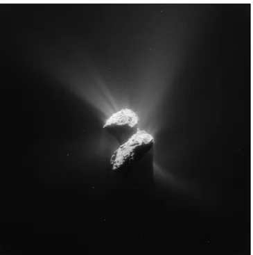
NEAR (Near-Earth Asteroid Rendez-vous) Shoemaker is a space probe launched by NASA on 17 February 1996 to study one of the largest Earth-crossing asteroids, Eros 433, shown in Figure 2.1. It was the first NASA Discovery programme mission, which contributed to several advances in the development of modern navigational strategies to manoeuvre a spacecraft around an irregular body.

The main objective of this 800 kg mass probe, including 56 kg of scientific instrumen-tation, was to identify the main features of Eros, such as its mass, internal distribution, magnetic field and mineralogical composition (Cheng et Andrew, 2002). To this end, the probe was launched on February 14, 2000, set in orbit around Eros and remained for around a year. The mission ended on 12 February 2001 when, even though it was not planned for such manoeuvres, the spacecraft landed. Against all odds, the spacecraft survived to the landing, and transmitted data and Until 28 February 2001.

Eros’ a-priori knowledge was not sufficient to allow an accurate design of the orbit, which could have led to unexpected disturbances during the mission, especially in this highly disturbed environment (Owen et al., 2002). The most powerful navigation tech-nique successfully used for the first time during this mission, was optical navigation via Landmark tracking. In addition to the range and radio-metric measurement, these data were used for the asteroid’s orbit determination process, gravity and shape modelling, and rotational rate estimation (Williams, 2002).

(22)

2.1. PAST ASTEROID MISSIONS

Figure 2.1: Picture of 433 Eros (Image Credit : NASA)

2.1.2 Hayabusa

Also known as MUSES-C (Mu Space Engineering Spacecraft), Hayabusa was a Japanese Space Agency (JAXA) space probe. The aim of the project was to research a tiny asteroid named Itokawa and to test new robotic techniques to carry back to Earth a soil sample of the asteroid.

The asteroid probe was launched in 2003, and in 2005 it met with Itokawa, shown in Figure 2.2. Due to the difficulty of navigation in a very low gravity environment, several unsuccessful landing attempts were made before a small sample was obtained. Contact with the probe was very difficult because of the great distance between the planet and the asteroid. Hayabusa carried a star-tracker, IMU and a two-axis Sun-aspect sensor for inertial measurements, as well as optical cameras, lidar, and laser-range finder (LRF) for relative navigation. A three-month approach was scheduled (Hashimoto

et al., 2010) after the rendezvous in August 2005. The on-board equipment could not

provide sufficient information to estimate the key physical parameters during this process, because of the poor gravity of Itokawa and because the approach was made on a straight line. Therefore, 3 km away from the centre of mass of the asteroid, an orbit phase was scheduled, requiring high navigation protection procedures to prevent collisions with the surface of the asteroid. Since Hayabusa moved towards the asteroid in a straight line, an accurate asteroid gravitational field estimation was not needed for navigation in the first mission phase (Yoshikawa et al., 2006). Instead an assessment of the solar radiation pressure and gravity in the trajectory was used to estimate the mass.

2.1.3 Rosetta

To analyse and collect data on the core composition of comet 67p/Chouriusumov-Guerassimenko, Rosetta was launched by the European Space Agency on 2 March 2004. This research

(23)

Figure 2.2: Hayabusa spacecraft and the asteroid Itokawa (Yoshikawa et al., 2006).

origin of the Solar system. Rosetta is the sixth spacecraft that observe a comet from a short distance, but the first to orbit a comet and carry a lander to the surface. On 12 November 2014, Philae landed on the surface. In many aspects, this project was a real technological challenge. Until the spacecraft met the target, the main parameters, the gravity and the physical parameters such as mass remain undetermined. As the trajec-tory was very difficult to forecast, because of this lack of knowledge, a versatile strategy to cover for the uncertainties had to be adopted. In addition, the probe had to be au-tonomous during critical phases, which is a real challenge for safety and navigational design, due to the substantial Earth-comet distance (Munoz et al., 2012). The trajec-tory of the spacecraft was estimated by radiometric monitoring from ground stations on Earth, such as the Doppler range or the DDOR (Delta-Differential One Way Range), which provided reliable data on the Solar System barycenter. However, this knowledge was not sufficient to describe the approach trajectory relative to the comet, primarily due to significant uncertainties about the comet and its environment (Godard et al.,2015).

Accurate relative navigation could only be achieved by using optical navigation meth-ods with on-board optical cameras taking pictures of the comet’s surface, defining direc-tions from Rosetta to the comet’s centre and enhancing relative navigation performance (Castellini et al., 2014).

2.1.4 Dawn

Dawn was a NASA probe launched in 2007, the mission of which was to study Vesta and Ceres, the two major bodies of the Main Belt. The observations began in 2011, first orbiting Vesta and then Ceres, and ended in 2018. It was the ninth mission of NASA’s Exploration Program. The DAWN mission was the first to use only optical navigation for relative navigation with radiometric and Doppler data for absolute navigation. No altimeters or star-trackers were used, only two navigation cameras (FCs) were carried for redundancy. Optical navigation cameras have been used for scientific purposes as well as for the orbit determination and gravity modelling (Konopliv et al.,2014).

(24)

Figure 2.3: Picture of the comet Tchouri taken by the NavCAMs of Rosetta, 5 June 2015. (Image Credit : ESA)

(25)

2.2. AUTONOMOUS NAVIGATION RESEARCH

2.1.5 Osiris-Rex

OSIRIS-REx (Origins-Spectral Interpretation-Resource Identification-Security-Regolith Explorer) is a NASA mission launched on September 8, 2016 to research and carry back a sample of the Earth-crossing asteroid named Bennu.

The main objective of this mission is to collect data that will allow us to better understand the Solar System’s formation process. The primary elements of the Solar System that the asteroid has retained can be isolated by retrieving a sample from the surface. It is the first mission by NASA to send an asteroid sample back to Earth. In terms of navigation and flight dynamics, this mission faced many difficulties, such as very accurate manoeuvring and orbiting around a very small asteroid, at low altitude, to precisely map the surface. The sample has been obtained by a robotic arm after landing on the surface, requiring surface navigation. The return to earth is expected to take place in 2023.

Launch and interplanetary phase navigation was made by Radio metric tracking using Nasa Deep Space Network and DDOR to estimate the absolute state of the spacecraft

(McMahon et al., 2018). The approach of Bennu was made by Optical Navigation

Track-ing and lidar, to estimate the relative state of the spacecraft with respect to the asteroid. During this mission, a new navigation technique called Natural Feature Tracking (NFT) was introduced and tested. To evaluate the trajectory, the NFT uses image analysis. It compares features previously determined during earlier stages of the missions with on-board data of known features during landmark tracking to assess the spacecraft’s attitude and uses extended Kalma, filter to update the position and velocity based on the previous spacecraft state.

2.2 Autonomous navigation research

Autonomous navigation is a very broad topic, as it covers all stages of the navigation process, from the sensors to the estimation technique. Numerous research has been carried out in this area, and it is still a very active research topic to study for future missions.

2.2.1 Current research objectives and results

The asteroid environment, while dominated by the gravitational field effect of this body, is generally a highly disturbed environment. As we have seen before, asteroids are usually small and may have very irregular shapes. These properties of asteroids contribute to a very complex dynamic system, which makes it very difficult to orbit around them. Orbits can be quite tough to anticipate and thus it is complicated to ensure safe navigation and prevent collisions with the surface. The interest in landing asteroids makes it even more difficult to ensure the safety of spacecraft. Moreover, since the shape and rotation of the asteroid are not known beforehand, the spacecraft must provide a complex and robust GNC system to approach, meet and land safely on the asteroid. That is why autonomous navigation is being studied for this kind of mission, to improve on-board knowledge and therefore improve navigation safety.

(26)

2.2. AUTONOMOUS NAVIGATION RESEARCH

Figure 2.5: Image of Bennu taken by polycams of Osiris-Rex mission before spacecraft arrival (Image Credit:NASA)

We should think of the work of Mooij et al. (2009), which studied the gravitational modelling of a diamond-shaped asteroid, Steins, for autonomous navigational purposes, and which is the main basis of this thesis. They have shown that the spherical harmonics model diverges near to the surface and therefore it is wiser to use a polyhedral shape approximation or a triaxial ellipsoid model. However, the last two models are seen to be 20 times slower than the spherical harmonics model.

Kubota et al.(2010) discuss an autonomous GNC system for the MUSES-C spacecraft

and the Rendez-vous and Landing Conditions. Gil-Fernandez et al. (2019) demonstrate HERA’s GNC technology, developed to maintain a balance between navigation safety, flight operations, payload and spacecraft characteristics and time constraints. The GNC system depends on a vision-based navigation system with a landmark tracking as well as an attitude-based approach. Autonomous navigation based on optical tracking is a very promising technique, particularly for asteroid landings. The new autonomous navigation algorithm for optical navigation is described in the work of Shuang et al. (2013), which achieved a position error and a velocity error of less than 1 m and 0.1 m/s respectively.

2.2.2 Msc Thesis heritage

The studies already done by fellow students at TU Delft have been reviewed to support our research. We can think of the work ofRazgus(2016), who used a dual-quaternion ap-proach to investigate the relative navigation in the vicinity of asteroids. He compared two separate approaches, the Cartesian coordinates for position and the attitude quaternions,

(27)

2.3. OUTCOMES, LIMITS AND INITIATIVES

and the double quaternions approach. The two methods, he concluded, were quite simi-lar. Some of the models that he developed will be reused in the future study, for example for the asteroid and its environment. We may also think of the study of Moreno Villa

(2018), which examined the motion of satellites around small bodies. A GNC simulator was designed to test the behaviour of the orbit determination methods used in ground control centres. The results showed a difference in magnitude between the long and cross-track directions and the radial direction, due to a lack of information on the line of sight of the optical measurements, which could not be removed. Both of these master’s thesis will be used as a basis for the development of our simulator, as they already developed a navigation software and simulator, and they both worked in asteroids environments.

2.3 Outcomes, limits and initiatives

Outcomes and drawbacks of navigation systems observed during previous missions will be evaluated in this section. The conclusions, assumptions and mission requirements that result from this analysis will be detailed.

2.3.1 Outcomes and Limits

Future asteroid missions would require a high degree of guidance, navigation and control autonomy to minimise costs and to perform more complex missions. During previous missions, different navigation strategies have been used. Near-Shoemaker faced a lot of navigation challenges due to the unusual shape of the asteroid. In addition to optical landmark tracking, it uses Radiometric Doppler and Range tracking to navigate around Eros. The SRIF filter was used to approximate the physical parameters of Eros, but the calculation of mass was quite difficult. Owing to the very low gravity of Eros, a high accuracy of navigation and low reaction time became very necessary to prevent escape or crash on the surface. As a result, the highly disturbed orbit at the time of the arrival at Eros was very hard to anticipate and the data was very slow to converge. Navigation camera images were analysed on Earth to identify landmarks, which makes this process very expensive in terms of workload and time loss.

Hayabusa encountered similar issues. The landmark tracking, which was processed on Earth, was a very heavy task for the navigation team. Navigation was intended to be entirely autonomous on the approach of Itokawa, but due to the malfunction of the reaction wheel and the complex shape of Itokawa, it was not possible to locate the centre of mass of the asteroid. Hybrid ground-based optical navigation was therefore used instead of autonomous navigation. Gravity simulation of Itokawa were carried out using periods of no thrust but the accuracy was poor due to the direct trajectory of the spacecraft.

Rosetta showed some weaknesses in the absolute navigation system. The star-trackers used to determine the absolute location of the spacecraft became disturbed by the debris of the comet and the increasing activity of the comet. Star trackers help monitor the attitude of the spacecraft by guiding the high-gain antenna to Earth for communication. Thus, as this condition arose, the high-gain antenna began to drift away from Earth, and communications with the spacecraft were almost lost. It has been demonstrated that star-trackers cannot function independently in such a noisy environment.

(28)

The initial Osiris-Rex mission was to use only Lidar for autonomous navigation, but a new system, a natural tracking feature, was added due to reliability issues. The NFT framework depends on the integration of images captured by optical navigation systems with an on-board catalogue. Since this device was brought late in the mission process, it was not completely used during this mission, but this system has an immense potential for future missions.

These missions have contributed to the development of many techniques essential for precise navigation. Kim et al.(2007) developed a Multiplicative Expanded Kalman Filter to approximate the relative state of the spacecraft with high precision, based on optical-navigation measurements. The outcome of this research is an estimate of the state of the asteroid as well as the state of the spacecraft. Many on-board optical estimation algo-rithms have been developed for small-body exploration, based on the results of previous missions and the shortcomings of current missions, such as the AIM mission. The impor-tance of autonomy has been emphasised, and the incorporation of camera measurements into the on-board spacecraft estimator has been a significant topic of past research. We should think of the work of Hashimoto et al. (2010), which uses the estimator for the asteroid return sample mission. Adding a laser range to optical navigation as with the Osiris-Rex mission, significantly improved navigation accuracy. The NFT can be used to lower the laser range error, which can be very high based on the shape of the asteroid.

2.3.2 Mission requirements

Missions requirements can be discussed according to the mission heritage information. REQ-MIS-01 433 Eros will be chosen as a reference asteroid for the thesis.

REQ-MIS-02 The asteroid will be visited by the spacecraft and the results will be compared to existing models built during the NEAR mission.

REQ-MIS-03 The spacecraft will be designed on the basis of the Near-Shoemaker space-craft, weighing 800 kg, with a cubic shaped body of 1.7 m length and two solar panels with dimensions 1.2 × 1.8 m.

REQ-MIS-04 The mission should be based on the Near mission. First, a flyby at 1200 km will be conducted to estimate the SRP and an a-priori of the µ parameter value, then a 200 km orbit to estimate µ more accurately, and to attempt the estimation of the J2 and first-order harmonics coefficients. At 50 km from the surface, an attempt

to estimated the spherical harmonics coefficients will be made and confirmed with a 35 km altitude orbit, who should terminate the estimation.

REQ-MIS-05 The trajectory should be designed to ensure maximum time with suffi-cient illumination conditions for optical navigation, i.e., the phase angle (the angle between the direction of the Sun and the spacecraft’s relative position vector) must remain within the range of 20◦ to 70◦.

REQ-MIS-06 The mission shall be planned to ensure optimum surface coverage, i.e., the inclination should be as near as possible to 90. In addition, repeat orbits must be avoided.

(29)

REQ-MIS-07 The spacecraft shall navigate autonomously without the intervention of the ground station.

REQ-MIS-08 The spacecraft is equipped with a star tracker for absolute attitude mea-surement.

REQ-MIS-09 The spacecraft is equipped with Lidar and optical navigation cameras for relative state measurement and the creation of a digital elevation model to characterise the surface of the asteroid.

REQ-MIS-10 The spacecraft carries an accelerometer to estimate the solar radiation pressure in the early characterisation phase.

REQ-MIS-11 The navigation system should be able to estimate the gravity field of the asteroid as well as its rotational rate and the inertial state of the spacecraft. REQ-MIS-12 The trajectory should remain a collision-free course at all times, which

means that the distance between the asteroid and the spacecraft cannot be less than the error on the state of the spacecraft.

REQ-SYS-01 The spacecraft should be able to navigate around an asteroid, regardless of its physical characteristics.

REQ-SYS-02 For optimum landmark navigation the phase angle should be constricted between 20◦and 70◦, that the surface seen by the camera is illuminated.

REQ-SYS-03 The mass of the asteroid and the SRP force shall be determined with a 3-sigma accuracy of at least 10%.

REQ-SYS-04 The state of the spacecraft should be estimated with a precision of 10 m for the position and 1 mm/s for the velocity, with 3-sigma confidence.

REQ-SYS-05 The gravity field coefficients should be determined at least up to the order/degree 8 with a 3-sigma accuracy of at least 10%.

REQ-MAT-01 The software should be able to run on a computer with the following characteristics: i5-6200U CPU, dual-core 2.30-2.40 GHZ, 8Go RAM. The simulation time should not exceed one day in total for each scenario.

2.3.3 Assumptions

The assumptions of the missions are the following :

• At the beginning, only the distance between the Earth and the asteroid is known, as well as a gross estimate of the mass and shape of the asteroid.

• The first part of the spacecraft’s trajectory, from the Earth to the asteroid’s en-counter, is not considered. This part of the journey is assumed to be well designed in advance, without any disruptive body encounter.

• The physical parameters of the asteroid remain unknown, until the spacecraft is close enough to determine those parameters by itself.

(30)

• The only perturbations present in the environment will be the SRP force and torques, the gravitational effect of the asteroid and the third-body perturbation from the Sun.

• In the Simulator, the gravity field of the asteroid will be modelled with a spherical harmonics model up to degree and order 22, with coefficients obtained from the NEAR mission.

• The SRP force is assumed to be estimated in the early characterisation phase with an accelerometer, the estimation will not be conducted in this thesis.

• After the early characterisation phase, the surface of the asteroid will be scanned and the landmarks will be identified. Their coordinates will be stored on-board for the next phases.

• The motion of the asteroid around the Sun will not be taken into account.

• We can assume a constant rotational rate for the asteroid, to be determined by the navigation process. No nutation or precession effects will be taken into account. • The spacecraft is able to navigate around asteroids only, comets being the source

of extra noise due to their geological activity.

• We will use ideal sensors, which means that the sensors have no scaling errors or misalignment

• No image processing will be done during the thesis. The navigation camera will output noisy pixel coordinates of landmarks.

• Only the estimation of the required states and parameters will be done. During this time, we assume that the position and velocity of the spacecraft will be au-tonomously controlled.

(31)

3

Asteroids

Asteroids, also called minor planets, are small bodies made up of rocks, metals and gazes, with lengths ranging from a few metres to hundreds of kilometres. While the origin of asteroids is still one of the most complex problems in cosmology, the prevailing hypothesis is that they are made up of residual fragments of the initial protoplanetary disc. They are therefore considered to provide valuable information about the genesis of the Solar System. This chapter will detail asteroid properties and their classification.

3.1 Physical and Dynamical Properties

The primary recognised feature of asteroids is their diversity. They vary in scale, form, colour, chemical and mineralogical composition from each other, which makes them so distinctive. This particularity makes asteroid missions much more complicated, since for navigation and trajectory design, the dynamic properties of the target object are very important.

3.2 Mass, Shape and Size

The Rosetta probe showed in detail the Tchouri Comet’s irregular structure and very steep surface. The Solar System is full of different shapes of these small celestial objects. However, some objects are almost spherical, such as planets, the Sun, or the Moon. This is mainly due to the fact that the electrostatic force of these bodies exceeds the gravitational force. Thus, their gravity field dominates the inner strength of the planets, which contributes to an equilibrium shape.

It is the electrostatic force that dominates a less massive object. However, its range is restricted to a few interatomic distances, unlike gravitational force. Therefore, it has no effect on the body’s overall form. This is why small celestial objects may have an irregular shape and thus an irregular gravity field, such as Tchouri, whose size is a few kilometres. It has been shown that an asteroid’s shape can also be influenced by spin rates (Holsapple, 2001) and distinguished from hydrostatic equilibrium. It is possible to observe different shapes of asteroids, as shown in Figure 3.1.

Mass estimation of asteroids is very important for enhancing the understanding of inner planetary motion. Typically, estimating the mass of an asteroid from ground-based

(32)

3.3. ROTATIONAL RATES

Figure 3.1: Various shapes of asteroids (Image credit: NASA)

measurements is very difficult and errors can be greater than 50%. Two key methods are used to estimate an asteroid mass from ground-based observation, a dynamic method and an astrophysical estimation method. The dynamical approach is based on observations of the impact of asteroid-related gravitational disturbances on other objects in the sur-rounding region of this asteroid. This method provides direct mass measurements and, as shown by Ivantsov and Anatoliy (2008), can lead to relative errors of less than 50%.

Another way to estimate the mass of the asteroid is to study the effect of the asteroid on a spacecraft during a mission. Optical observations, Doppler and range measurements of the spacecraft orbiting can be used to calculate the mass of the asteroid as shown by

Yeomans et al. (2000) during the Near Shoemaker mission. The mass can also be

deter-mined by observing the effect of the asteroid on the predicted trajectory. As shown by

Yeomans et al.(1998), during the flyby of 253 Mathilde by the Near-Shoemaker spacecraft,

the impact of the gravitational disturbance on the spacecraft was sufficient to estimate the mass using the tracking data. Using the optical data collected from navigation cam-eras, an estimate of the volume can be made when the spacecraft is close enough to cover the whole body with the cameras. The volume can also be determined by astronomical infrared measurements. It makes it possible to estimate the so-called bulk density of the asteroid. Asteroid bulk density measurements may provide insight into the internal structure or porosity of the object.

3.3 Rotational rates

Study of the rotation of asteroids is essential in understanding the structure and for-mation of asteroids. Celestial bodies rotate due to the accumulated angular momentum during their creation and the additional angular momentum due to collisions with other

(33)

3.3. ROTATIONAL RATES

Figure 3.2: Asteroids spin rate vs diameter plot (Hughes, 1983).

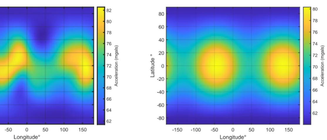
bodies. Rotational rates also have a major impact on the orbiting spacecraft, which is why knowledge of this rate is critical for navigation and trajectory design. In addition to light-curve results, rotation studies provide details on the internal structure of the aster-oid. Although several studies have been performed in this area, the understanding of the relationship between asteroid properties and rotational speeds is still not well understood. Many asteroids rotate uniformly and have a rotation period ranging from very fast (T = 1.3 min) to very slow (T = 2.400 hours). Hughes (1983) has shown that there is a relationship between the rotational rate and the size of the asteroid, as shown in Figure

3.2. The bold solid curve is the geometric mean spin rate vs. diameter, the thin solid curve is the limit used to exclude slow rotators. Constant time-scale damping lines of non-main-axis rotational motion (thin dotted lines) are also plotted. From this figure, we can see that increasing the diameter causes the mean rotational rate to decrease.

As written by Pravec and Harris (2000), the population of asteroids can be distin-guished. It has been shown that there is a limit in the spin rate for asteroids with a diameter greater than 40 km, which I s approximately 2.4 hours. This limitation can be explained by the fact that most of these asteroids are made up of rubles that will break apart at higher spin speeds. There are two distinct populations of asteroids smaller than 40 km in diameter, slow and quick rotators. For the smallest asteroids with a diameter of 0.15 km the spin rate can be very high, up to 1.3 min and can be understood by their monolithic composition. Among Near Earth asteroids, a significant fraction of the fast rotators are binary systems. They are probably the product of the disturbance of the tidal waves during their passage near planets.

The composition of asteroids may also have an influence on their rotation period. Indeed as Harris and Burns (1979) indicates, Type-C asteroids have a rotation time of 20% slower than Type-S asteroids. This indicates that C-type asteroids are less compact

(34)

3.4. CLASSIFICATION

or less dense than other types. While most asteroids have one main axis of rotation, a small fraction of them have an additional axis of rotation that can be correlated with precession and nutation effects, and this can lead to unexplained rotations such as the Toutatis asteroid. Its rotation is the product of two distinct forms of motion around two axes with a period of 5.4 and 7.3 Earth days respectively. Its shape and its specific rotation could be the result of several collisions.

3.4 Classification

Asteroids can be categorised using their distribution within the Solar System, their chem-ical composition and configuration.

3.4.1 Spatial location

Main groups of asteroids based on their locations within the Solar system are:

The Main Belt of Asteroids: Between the orbits of Mars and Jupiter, the largest group of asteroids in our Solar System is located at a distance of two to four astro-nomical units (au). Around 720,000 objects from this belt have been listed so far (2019). Due to orbital resonance phenomenon, the impact of the gravitational field of Jupiter has stopped all these bodies from forming a planet and is the source of the Kirkwood gaps, almost empty areas found in the middle and on the edges of the belt.

Jupiter Trojans: Trojan asteroids share their main body’s orbit around the Sun, and are centred around the Sun-Jupiter system’s L − 4 and L − 5 Lagrange points. In the region of Jupiter, the largest Trojan asteroids are found, hence the name of the Jupiter Trojans.

Near Earth asteroids (NEAs): Asteroids with an orbit similar to the orbit of the Earth with a radius of perihelion equal to or less than 1.3 au. Earth-crossing asteroids (ECAs) are asteroids with a radius of aphelion equal to or less than 1,381 au (Mars-Sun distance) and whose orbits cross the orbit of the Earth. Potentially Dangerous Asteroids (PHAs) are a specific and significant class of NEAs for which the trajectory passes very close to Earth and could cause catastrophic damage to the Earth.

Centaures: They are known to be minor planets that gravitate between the Gas Giants’ orbits. Owing to the intense impacts of the outer planets, they usually have unstable orbits.

Kuiper Belt and trans-Neptunian objects: There are asteroids whose orbit is be-yond the orbit of Neptune. The Kuiper belt is a ring similar to the Main Belt located in the trans-Neptunian zone, but much broader, wider and much more mas-sive. It is mainly made up of bodies of small sizes and three dwarf planets, Pluto, Makémaké, and Hauméa.

(35)

3.5. INTEREST IN 433 EROS

3.4.2 Chemical composition

The composition of the asteroids is assessed, as written by Shestpalov and Golubeva

(2020), according to their optical spectra measuring the reflected light. This classification scheme is called asteroid spectral classification. Even if the chemical composition of the asteroids is very complex, depending on their mineral composition, it allows the asteroids to be divided into different groups. The following are the primary types:

• C-Type asteroid: The most common known asteroids (around 75%) are carbona-ceous asteroids. They are distinguished by a very dark colour and their structure, without light and volatile elements such as ice, is similar to the primitive Solar System.

• S-Type asteroids: They are mostly composed of silicates, which are moderately white and composed primarily of iron, magnesium and nickel. They are the second most common type, with 17% of the known asteroids.

• M-Type asteroids: They have a composition that is partly known and corresponds to the rest of the asteroids. They are distinguished by a bright surface, and some of them are often made of an iron-nickel alloy.

3.4.3 Configuration

Asteroid configuration helps us to classify them into three categories: single asteroids, binary asteroids contact, and binary asteroid systems. The configuration affects the as-teroid’s shape, which can be from very irregular to nearly spherical. Single asteroids are bodies with only one element and their irregular shapes define them. They constitute 20% of the Solar System’s asteroids. Binary systems are the composition of a primary aster-oid and a secondary asteraster-oid, orbiting around their common barycenter .They constitute roughly 17% of the NEAs. Finally, contact binaries are binary systems whose compo-nents have gravitated towards each other before direct physical contact was formed. It is possible to perceive them as a single body consisting of two lobes. Since most asteroids are irregularly shaped, predicting their gravity field is very difficult. They can be pitted or crated on the surface and that is why it is necessary to know their characteristics in detail to ensure secure missions

3.5 Interest in 433 Eros

433 Eros was discovered on August, 13, 1898 by August Charlois, in Nice, France, and by Gustave Witt, in Berlin, Germany. It is a Near-Earth asteroid, meaning that its orbit is approaching or crosses the orbit of the Earth. It is very useful to understand this class of asteroids and in particular, potentially hazardous objects (PHOs) to anticipate and prevent possible Earth impacts. From a chemical point of view, Eros primarily consists of silicates and thus belongs to asteroids of type S. It belongs to the group of Amors, also known as Earth-grazing asteroids, a group of small bodies which do not cross the Earth’s orbit. Eros is following an elliptical trajectory, with a 1.13 AU perihelion and a 1.78 AU aphelion. The trajectory is inclined of 10.8◦with respect to the ecliptic, with an average 21

(36)

3.5. INTEREST IN 433 EROS

Table 3.1: Characteristics of 433 Eros

Size 33 km x 13 km x 13 km

Approximate mass: 7.2 × 1015 _kg

Rotation Period: 5.270 hours Orbital Period: 1.76 years Spectral Class: S

Semi major Axis: 1.458 AU Perihelion Distance: 1.13 AU Aphelion Distance: 1.78 AU Orbital Eccentricity: 0.223 Orbital Inclination: 10.8 deg Geometric Albedo: 0.16

distance from the Sun of 1.46 AU1. The general characteristics of Eros are resumed in the Table 3.1. All the data collected during the NEAR mission, such as shape, gravity models, and landmark data are available on a dedicated website.2.

The (NEAR)–Shoemaker mission was a breakthrough in that it reflected the realistic navigation of a spacecraft in the most seriously disturbed orbital environment a spacecraft has ever encountered. In addition, all future asteroid orbital missions will encounter conditions close to those experienced by NEAR at Eros in some way. It is therefore very interesting to take this asteroid as a reference for this study, particularly since its highly irregular shape contributes to a highly irregular gravitational field, and therefore the modelling of this gravitational field could be a very tough challenge. In addition, numerous models are currently available for the Eros shape and gravity field, which can be used as a reference for the results obtained during this thesis.

1_{https://nssdc.gsfc.nasa.gov/planetary/text/eros.txt Accessed on: 27-04-2020}

(37)

4

Orbital Mechanics and Flight

environment

The asteroid environment and spacecraft dynamics will be presented in this section. It will reveal the technical characteristics of the spacecraft to be used in the simulator, as well as the properties of the asteroid and the disturbing forces that can encounter the spacecraft around this kind of body. The Near-Shoemaker mission will be used as a reference for this thesis, so we will be studying the asteroid 433 Eros.

4.1 Spatial representation

Details on the reference frames and coordinate systems used to describe positions and attitudes in the real environment will be provided in this section.

4.1.1 Reference frames and Cartesian coordinates

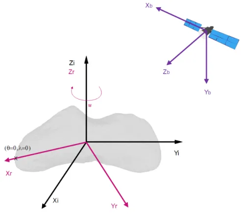
The motion of the spacecraft and the asteroid in the environment is represented by three reference frames, from which the Cartesian coordinates can be obtained, as shown in Figure4.1:

“Inertial” reference frame: It is a rotating frame and is assumed to be non-accelerating with respect to the stars’ reference frame, originating at the asteroid’s centre of gravity. The X-axis is set by use of the vernal equinox. This reference frame is used both to explain Eros’ rotation and to describe the spacecraft’s inertial state. In this reference frame, the coordinates are denoted by (xI, yI, zI).

Asteroid reference frame: This reference frame, since it rotates with the asteroid, is non-inertial. It is again fixed to the asteroid’s centre of gravity, but with the X-axis fixed to the asteroid’s prime meridian, selected by Near scientists, and equator, and the Z-axis parallel to the axis of rotation. The prime meridian defines the zero-degree longitude line, while the equator defines the zero-zero-degree latitude line. This reference frame is used to describe, with respect to the asteroid, the relative state of the spacecraft. The coordinates in this reference frame will therefore be denoted as (xR, yR, zR).

(38)

4.1. SPATIAL REPRESENTATION

Figure 4.1: Reference frames

Body Reference frame: This reference frame is fixed to the spacecraft, with the axis coinciding with the principal inertial moments. The Z-axis is aligned with the line-of-sight of the camera, and parallel to the solar panels is the X-axis. This reference frame is used to explain both the rotational motion and the pointing of the instruments of the spacecraft. The coordinates are denoted by (xB, yB, zB) in

this reference frame.

4.1.2 Sphere-based coordinates

In addition to Cartesian coordinates used to describe the motion of the spacecraft, sphere-based coordinates are used. These coordinates are fixed to the asteroid system, which means that they are rotating with the asteroid, and are thus determined with respect to the reference frame of the asteroid, as shown in Figure4.2. The two systems of coordinates are:

Spherical coordinates: Consisting of three components, the distance d, the colatitude Φ, the angle between the position vector of the Z-axis and the position vector of the spacecraft, and the latitude λ, the angle between the prime meridian and the position vector projection of the X-Y plane. A triple (d, Φ, λ) can define the coordi-nates of the spacecraft. This coordinate system enables the asteroid’s gravitational field to be computed in a much simpler way.

(39)

4.1. SPATIAL REPRESENTATION

Figure 4.2: Spherical and geographic coordinates system

Geographical coordinates: Represented by the (θ, λ) pair, the geographical coordi-nates provide information on the relative location of the spacecraft projection on the asteroid surface. θ is the angle of latitude, and λ is the angle of longitude. This method is very useful when the asteroid is rotating, to determine the force acting on the spacecraft due to the highly irregular gravity field of the asteroid.

4.1.3 Frame transformations

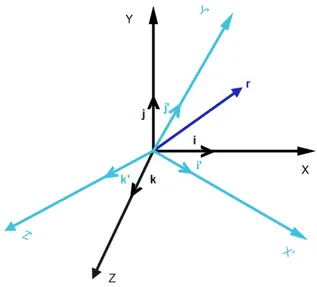
We will need to switch from one reference frame to another in the simulator. This can be done by using a transformation matrix, which enables a vector to be transformed from the perspective of the old reference frame to the new one. The transformation does not alter the vector itself but changes its components to preserve its representation in the new reference frame.

If we consider a (X, Y, Z) reference frame, called A, to which we apply an arbitrary axis rotation, the resulting frame (X0, Y0, Z0), called B, is shown in Figure 4.3. We can write the vector coordinates in the new reference frame, that is:

rX0 = r · i0 = (r_Xi + r_Yj + r_Zk) · i0 = r_Xi · i0+ r_Yj · i0 + r_Zk · i0

rY0 = r · j0 = (r_Xi + r_Yj + r_Zk) · j0 = r_Xi · j0 + r_Yj · j0 + r_Zk · j0

rZ0 = r · k0 = (r_Xi + r_Yj + r_Zk) · k0 = r_Xi · k0+ r_Yj · k0+ r_Zk · k0

(4.1)

(40)

4.2. ASTEROID ENVIRONMENT

with (i, j, k) and (i0, j0, k0) the unit vector of the original and rotated reference frame respectively. These equations can be written in a more compact way, that is:

  rX0 rY0 rZ0  =   i · i0 j · i0 k · i0 i · j0 j · j0 k · j0 i · k0 j · k0 k · k0     rX rY rZ  = TB/A   rX rY rZ   (4.2)

with TB/A the transformation matrix from the reference frame A to the reference frame

B. The inverse transformation can be applied by:   rX rY rZ  = TA/B   rX0 rY0 rZ0   (4.3) where: TA/B = TTB/A (4.4)

Using the direction cosine matrix (DCM) is another way of computing the rotation from a reference frame to another. The unit vectors of the B reference frame, in the A reference frame, can be written as:

i0 = cos θ11i + cos θ21j + cos θ31k

j0 = cos θ12i + cos θ22j + cos θ32k

k0 = cos θ13i + cos θ23j + cos θ33k

(4.5)

where the θij corresponds to the angles between the corresponding unit vectors, as shown

in Figure 4.4. Therefore:   rX0 rY0 rZ0  =  

cos θ11 cos θ2 cos θ31

    rX rY rZ  = CB/A   rX rY rZ   (4.6)

The direction cosine matrix CB/A, which represents the attitude of the B-frame in relation

to the A-frame, can be used to transform a vector from a reference frame to another frame.

4.2 Asteroid Environment

During the NEAR mission, a spherical harmonics model of the shape and gravity field of 433 Eros was made by Miller et al. (2002). Using radiometric tracking data, optical images and the NEAR laser rangefinder (NLR) to determine the shape, rotational rate and gravity field of Eros, NEAR spacecraft were injected into many different orbits. To determine a 24th degree and order shape model, the NLR and optical data from a 50 km altitude orbit were used. In parallel, the radiometric data, together with the optical data, were used to in the orbit determination process determine the gravity field of Eros up to 15 degrees and order, from a 35 km altitude orbit. The shape model integration given by the NLR shape model, assumed a constant density. Since the results of this model are very close to those obtained by the orbit determination process, it indicates

(41)

Figure 4.3: Rotation of a reference frame around an arbitrary axis

Figure 4.4: Direction cosines angles

that the density of Eros is almost uniform on a large scale (1% variation for 35 km). After the mission, the data collected was post-processed to create more precise models, such as the Chanut et al. (2014) polyhedron shape model and the Garmier et al. (2002) ellipsoid model. To determine stable orbits around Eros, the polyhedron model was used, as shown in Figure 4.12a. Chanut et al.(2014) has identified a minimum radius of 36 km for direct, equatorial and circular stable orbits and a minimum radius of 31 km for any other stable orbit. Only in elliptical orbits can be found stable at lower altitudes.

(42)

4.2.1 Asteroid gravity field

Asteroids are defined by their complex shape and limited size. This feature, along with the rotational speed of the asteroid, contributes to a complex dynamic situation in the vicinity of asteroids. The gravitational field is relatively weak, but as it is the main source of disturbance near the surface of the asteroid, gravitational disturbances can be very large. They can lead to substantial deviations in the nominal trajectory of a spacecraft. Awareness of this gravitational field may also provide details about the inner structure and mass distribution of the celestial body.

Due to the large perturbations, the spacecraft would face high risks of collision with the surface of the asteroid, if the gravitational field is not modelled correctly. Two models are generally used to model the gravitational field of such bodies, polyhedral modelling and spherical harmonic expansion. Those models have been studied by Werner and

Scheeres(1996) who came to the conclusion that polyhedron model was the most accurate

model, while harmonics modelling suffered from convergence and accuracy problems. An ellipsoidal harmonic expansion can also be used, as written by Garmier et al. (2002), to model the gravity fields of asteroids with an elongated shape. For Eros, this model leads to more accurate results.

This section will explain the various ways of modelling an asteroid’s gravity field, and will provide the gravity field model of Eros with details about the accuracy of these methods and their performance.

Point Mass approximation

The simplest way to model the gravity field of a body is to use the point mass approxima-tion. As Newton’s Law of Gravitation states, the gravitational force between two point masses distant in the vacuum, is an attractive force and can be written as proportional to the masses and inversely proportional to the square of the distance between the two point masses:

FP /Q = G

mPmQ

d2 eP Q (4.7)

with FP /Q the force acting on the body Q, by the body P , mP and mQ masses of the two

bodies, eP Q the unit vector in the direction of the centre of mass of the body 2, and d

the distance between the two masses.

Using the second law of Newton, we can write the gravitational acceleration a due to body Q acting on a body P :

a(P ) = −GmQ

xP − xQ

|xP − xQ|3

(4.8) where xP, xQ are the position vectors of the bodies P and Q, respectively.

If multiple bodies are in the spacecraft environment, the summation of all the individ-ual accelerations enables the identification of the total field strength. This representation is not very accurate, since it does not take into account the effect of the shape of the bodies on the gravitational field, but still yields a good approximation, especially when the bodies are far from the spacecraft. If we consider a volume mass, integrating all the elements dm = dΩ makes it possible to find the gravitational field of this volume.

Autonomous estimation of the gravity field for asteroids missions

SCHOOL OF ENGINEERING

Forl`ı campus

-SECOND CYCLE MASTER’S DEGREE in AEROSPACE

ENGINEERING

Classe LM-20

GRADUATION THESIS in Aerospace Equipments and Systems

Autonomous estimation of the

gravity field for asteroids missions

CANDIDATE:

Aur´

elia Bourgeaux

SUPERVISORS:

Erwin Mooij

Bart Root

Marco Zannoni

Abstract

Preface

Contents

Nomenclature

1

Introduction

1.2

Research questions

1.3

Thesis outline

2

Mission heritage

2.1

Past Asteroid missions

2.1.1

Near-Shoemaker

2.1.2

Hayabusa

2.1.3

Rosetta

2.1.4

Dawn

2.1.5

Osiris-Rex

2.2

Autonomous navigation research

2.2.1

Current research objectives and results

2.2.2

Msc Thesis heritage

2.3

Outcomes, limits and initiatives

2.3.1

Outcomes and Limits

2.3.2

Mission requirements

2.3.3

Assumptions

3

Asteroids

3.1

Physical and Dynamical Properties

3.2

Mass, Shape and Size

3.3

Rotational rates

3.4

Classification

3.4.1

Spatial location

3.4.2

Chemical composition

3.4.3

Configuration

3.5

Interest in 433 Eros

4

Orbital Mechanics and Flight

environment

4.1

Spatial representation

4.1.1

Reference frames and Cartesian coordinates

4.1.2