The Effects of Age and Job Protection on the Welfare Costs of Inflation and Unemployment: a Source of ECB anti-inflation bias?
Leonardo Becchetti Stefano Castriota
Osea Giuntella Abstract
This paper extends the well known Di Tella et al. (2001 and 2003) analyses on the welfare costs of inflation and unemployment based on self-reported happiness data by looking at age and job market characteristic splits in a sample which includes more recent years and new countries. With both one and two stage estimating procedures we find support for the hypothesis that the relative welfare cost of unemployment versus inflation is higher than one (in contrast with the “equal-to-one” implicit assumption of the Misery Index). We also observe that the relative cost of unemployment is much higher in intermediate age cohorts and in low job protection countries. This might contribute to explain the higher concern for the level of economic activity of central bankers in countries with younger population and more flexible labour markets.
Keywords: Phillips curve, unemployment/inflation trade-off, happiness, job protection, aging population
JEL Numbers:
* We wish to thank Michele Bagella, Marcello De Cecco, Filipa Sa and Marika Santoro for their useful comments and suggestions. The usual disclaimer applies.
1. Introduction
Evaluating the relative cost of unemployment versus inflation is of foremost importance for economists and policymakers1. In order to maximize the population’s welfare it is fundamental to know which one, between inflation and unemployment, has the highest impact on people’s lives. The effectiveness of economic policies is usually evaluated on the basis of welfare indicators which arbitrarily assign certain weights to the two bads. The most famous is probably the so called “Misery Index”2 which calculates countries’ well being levels with a simple unweighted sum of the unemployment and inflation rates. Its implicit (and strong) assumption is that a one percent rise of inflation and unemployment generate the same welfare loss.
0ne of the most influential papers in this literature (Di Tella et al., 2001) shows that the Misery Index underestimates the relative cost of unemployment. With a two stage approach the authors demonstrate that policymakers should trade off a one percent reduction in unemployment with a 1.66 percent increase of inflation in order to maintain constant the level of welfare. This finding contradicts the Misery Index hypothesis that the two “bads” have to be considered as perfect substitutes.
A main point of the paper is that the cost of unemployment is higher also because it does not affect only unemployed individuals. In fact, the latter is given by the sum of two components: the psychological cost of being
1 The discussion on the unemployment-inflation trade-off is probably one of the oldest and most controversial in the economic discipline. Is the Phillips curve really vertical in the long run? Is it linear or non-linear? Akerlof, Dickens & Perry (1996) challenge the traditional view on optimal inflation arguing that a moderate rise in the price level provides some “grease” to the price and wage setting process. Their study on the US economy suggests the existence of an optimal non-zero inflation rate, between 1.5% and 4%. Wyplosz (2001) finds evidence that the Phillips curve rates of inflation above 2%. “Sand” and “grease” effects differ among countries with different in the long-run is non-linear and not vertical. Furthermore, unemployment seems to decline for labour market structures. In particular Wyplosz, estimating the Phillips curve for Germany, France, Italy, Netherland and Switzerland, concludes that there may be a “sand effect” for low levels of inflation. For countries like Germany, higher levels of inflation (between 4% and 10 %) would be necessary to produce the “grease effect”. By combining these findings with the relevance of near rationality and the possible existence of nominal rigidities, Dickens (2001) claims that an inflation target below 2% could be very costly.
2 The Misery Index has first been used by Robert Barro in the 1970's, although some people credit it to Arthur Okun. It is simply the sum of unemployment and inflation rates. Both unemployment and inflation create economic and social costs, which are captured by a rise in the Misery Index.
unemployed (which affects only jobless people)3 and the general population fear of unemployment (which affects the whole population). The different statutes and behaviors of economic institutions in the US and Europe do not seem to reflect citizens’ superior concern for unemployment revealed by empirical evidence.
Several differences emerge when comparing the main targets declared in the statutes of the ECB and the Federal Reserve. The EU has found strong consensus for the creation of an independent Central Bank with a clear anti-inflationary stance and no explicit consideration of an unemployment target. The statute of the Federal Reserve, instead, lists six main monetary policy objectives, does not fix any clear inflation target and claims that the monetary policy should sustain economic growth and fight price increases at the same time.
When considering the Misery Index or the conduct of the central bankers, two questions arise. First, why do economic authorities implicitly have an antinflationary bias with respect to relative preferences of individuals as measured by the above mentioned studies? Second, why are there marked differences across countries in targets and policies (e.g. ECB versus FED)4? Our paper may help to solve the second puzzle. Our argument is that only by estimating the relative welfare costs of unemployment and inflation by
3 Clark & Oswald (1994), using data from the British Household Panel, show that unemployed people have much lower levels of mental well being than those at work. Controlling for age groups they find a negative relation between unemployment costs and the share of unemployed people in a given age cohort. This could reflect the fact that young people consider less stressful being unemployed, which could partly be explained by the reference-group theory. People tend to evaluate their status with respect to persons of their reference-group. L. Winkellmann & R. Winkellmann (1998), using panel-data (German Socio-Economic Panel), measure the effect for different age groups and find that older workers experience substantial reductions in satisfaction although they cannot reject the hypothesis that the detrimental effect of joblessness is the same across age-groups. There is also some evidence that being unemployed is easier when one has been out of job for some time or if one lives in a region with high unemployment (Clark & Oswald, 1994). Feather (1990) and Darity & Goldsmith (1996) provide an excellent review of the studies which have most contributed to theorize the relation between unemployment and psychological well-being.
4 De Grauwe (2005) evidences two main reasons for the ECB’s more conservative approach. The first has to deal with the Monetarist Counterrevolution, the emphasis put in the 80’s on the central bank’s independence (Barro-Gordon, 1984) and the call for a more conservative central banker (see Rogoff, 1985). The second refers to the role played by Germany in shaping the EMU and the Eurosystem.
different age and job market characteristic splits we may outline differences in preferences and political pressures observed on economic authorities. Using individual observations from the Eurobarometer Survey (1975-2002) we find that the relative individual cost of unemployment versus inflation is markedly higher in central age classes and in countries with lower job protection (JP).
Looking at these results we may infer that the progressive aging of the European society and its higher job market rigidity have progressively increased the constituency of those groups (retired workers, insiders with high job protection or even unemployed with high welfare provisions) which downweight the relative cost of unemployment versus inflation. This should be much less the case in countries with higher job market flexibility and younger population.
Even though our data cover only EU countries, the observed findings on the relatively higher psychological cost of being unemployed and the general population fear of unemployment in EU countries with lower job protection lead us to infer that also other countries with similar features, such as the US, should share stronger political pressure for more active anti-unemployment policies.
Our results may therefore help to understand why the much stronger population fear of unemployment may have contributed as well to the decision of countries with lower job protection, such as the UK, not to be part of the MU and countries like the US to shape the conduct of its central banker in a substantially different way.
The paper is divided into six Sections (including introduction and conclusions). In Section II we describe our variables, the methodology adopted in the two stage approach and the results obtained in terms of coefficient magnitudes and relative welfare costs of unemployment versus inflation. In Section III we perform robustness checks by running one stage regressions for different subsamples and one stage regressions with slope-dummy variables. In Section IV we perform further robustness tests by running a unique one stage regression in which age and job market characteristic effects are interacted. For every type of robustness check we derive the implied inflation/unemployment trade-off either in monetary terms or by considering relative changes in the share of very happy people. In Section V we discuss how demographic and structural variables might shape the institutions and their policies. Section VI concludes.
2. Data, variables and two stage econometric methodology
In building our database we closely follow the methodology used by Di Tella, McCulloch and Oswald (2001 and 2003) in order to make our results comparable with theirs. Our source is the Eurobarometer Survey containing information on self reported life satisfaction5 of more than 634,000 individuals from 1975 to 2002. With respect to Di Tella et al. (2003) we extend our analysis beyond 1992 and include new countries (Norway from 1990 to 1996, Finland from 1993, Sweden and Austria from 1994). Macroeconomic data are extracted as three year moving-averages centered in t-1 in order to reduce possible measurement errors. The source of unemployment rates is the OECD Center for Economic Performance dataset, while data on inflation are from the World Bank’s World Development Indicators.
5 Happiness and life satisfaction can be considered as synonymous as they generally provide the same regression results (see Di Tella et al., 2001). In our analysis we use the two words indifferently but always use the Life Satisfaction variable because it provides more observations than the Happiness one. The literature on the determinants of happiness is a new promising field of research and an important empirical benchmark on which the standard behavioural hypotheses on the homo oeconomicus utility function can be tested. Its revival after the reflection of the classics (see among others Malthus, 1798; Marshall, 1890; Veblen, 1899; Dusenberry, 1949 and Hirsch, 1976) is due to the emergence of international cross-sectional and panel datasets in which self declared happiness and life satisfaction are measured at individual level. For a survey on this branch of the literature see Frey and Stuzter (2002). On the plausibility and reliability of empirical findings based on self declared happiness data see, among others, Alesina et al. (2004). A remarkable element of the wide range of empirical papers on the issue is the stability across periods and countries of the relationship between self declared happiness and some of its determinants (see Alesina et al. (2004) for US and Europe, Frey et al. (2000) for Switzerland and Clark and Oswald (1994) for the UK).
Table 1: Description of the variables used
Name Source Variable
Life satisfaction Eurobarometer Self-declared life-satisfaction level from 1 (not at all satisfied) to 4 (very satisfied) Unemployed Eurobarometer Dummy variable (DV) which takes value 1 if the respondent is unemployed, 0 otherwise Selfemployed Eurobarometer DV which takes value 1 if the respondent is self-employed, 0 otherwise Retired Eurobarometer DV which takes value 1 if the respondent is retired, 0 otherwise Student Eurobarometer DV which takes value 1 if the respondent is student, 0 otherwise
Home Eurobarometer DV which takes value 1 if the respondent is responsible for home and is not working, 0 otherwise Male Eurobarometer DV which takes value 1 if the respondent is male, 0 otherwise
Age Eurobarometer Age of the respondent in years Age squared Eurobarometer Square of the respondent's age in years
Middle education Eurobarometer DV which takes value 1 if the respondent has 15-18 years of education, 0 otherwise High education Eurobarometer DV which takes value 1 if the respondent has more than 18 years of education, 0 otherwise Married Eurobarometer DV which takes value 1 if the respondent is married, 0 otherwise Divorced Eurobarometer DV which takes value 1 if the respondent is divorced, 0 otherwise Separated Eurobarometer DV which takes value 1 if the respondent is separated, 0 otherwise Widowed Eurobarometer DV which takes value 1 if the respondent is widowed, 0 otherwise Income 2nd quartile Eurobarometer DV which takes value 1 if the respondent belongs to the 2nd income quartile, 0 otherwise Income 3rd quartile Eurobarometer DV which takes value 1 if the respondent belongs to the 3rd income quartile, 0 otherwise Income 4th quartile Eurobarometer DV which takes value 1 if the respondent belongs to the 4th income quartile, 0 otherwise GDP per capita (2000
US$) World Bank GDP per capita in 2000 constant US $ Inflation World Bank Inflation rate, three-year moving average Unemployment OECD Unemployment rate, three-year moving average
We start our analysis by replicating the two stage procedure performed by Di Tella et al. (2001) with data from 1975 to 2002. In the first stage we regress the self-declared level of life satisfaction on a set of personal characteristics, on year and country dummy variables. We then calculate the average prediction error from the first stage by year and by country: we obtain an (unbalanced) panel of “unexplained” life satisfaction where every country has one observation per year. In the second stage we regress this newly created variable on the three-year moving average inflation and unemployment rates, year and country dummy variables and a country-specific time trend. More formally, in the first stage we estimate the following regression:
1
K
ijt j t k kijt ijt ijt
k
H α λ β X γU ε
=
= + + + + (1)
where Hijt is the happiness level of individual i living in country j in period t,
α
j andλ
t are respectively country and year dummy variables, Xk thek-th control variable in k-the individual happiness estimates and U ijt is a
dummy variable which takes the value of 1 if the individual is unemployed and 0 otherwise. Country unemployment and inflation rates are obviously excluded from the Xnjt controls. In the second stage we estimate the
following equation: 1 M jt j t jt jt jt m mjt jt m TREND u Y v η ϖ ϑ δ ψπ ϕ µ = = + + ⋅ + + + + (2) Where = i ijt jt i ε
η is the average unexplained residual for country j at time t from the first stage individual happiness equation,
ω
j
andθ
t
are respectively country and year dummy variables, TRENDjt is a linear trend(centered in t-1), jt and
u
jt are the three-year moving-average inflation and unemployment rates,Y
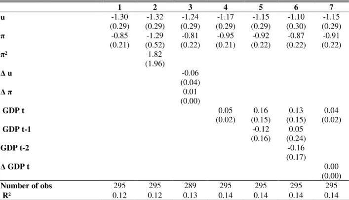
m is the m-th control variable (e.g. change in unemployment and inflation rates and current and lagged levels of GDP). In the first stage we use exactly the same regressors (with the exception of the number of children, not available after 1988) as in Di Tella (2001). The obtained findings are very similar: the coefficient of the unemployment status is -.34 against the -.33 of Di Tella 2001 (See Table 3, column 1). In the second stage we aggregate residuals from the first stage regression for each country-year and estimate the impact of inflation rates and aggregate levels of unemployment on satisfaction. In the base model with year and country dummies our second stage coefficients measuring the effects of unemployment and inflation are smaller than in Di Tella (2001): -1.3 against -2.0 for unemployment and -.85 against -1.4 for inflation (Table 2, column 1).After these first overall sample estimates we investigate if our results change when considering age cohort and job market characteristic splits.
We perform, in the first stage, one regression for each category6. Then, we calculate the average prediction error for every country-year by category and use these data to perform separate second-stage regressions by sample split 7. As age cohorts we consider the 25th (28 year old) and the 50th (41 year old) percentile of the age of sample respondents at the beginning of the investigation period. We divide the remaining 50% of the sample by taking into account the 65 year threshold which should discriminate between active population and retired workers.
Table 2: Two-Stage Life-Satisfaction Equations for Europe 1975-2002
1 2 3 4 5 6 7 u -1.30 -1.32 -1.24 -1.17 -1.15 -1.10 -1.15 (0.29) (0.29) (0.29) (0.29) (0.29) (0.30) (0.29) -0.85 -1.29 -0.81 -0.95 -0.92 -0.87 -0.91 (0.21) (0.52) (0.22) (0.21) (0.22) (0.22) (0.22) ² 1.82 (1.96) u -0.06 (0.04) 0.01 (0.00) GDP t 0.05 0.16 0.13 0.04 (0.02) (0.15) (0.15) (0.02) GDP t-1 -0.12 0.05 (0.16) (0.24) GDP t-2 -0.16 (0.17) GDP t 0.00 (0.00) Number of obs 295 295 289 295 295 295 295 R² 0.12 0.12 0.13 0.14 0.14 0.14 0.14
Legend: Second-stage regression results of the model presented in section 2 (see equation 2). The dependent variable is the country average of individual unexplained life satisfactions (the country average residual of equation 1 in section 2). Standard errors are in parentheses. Inflation and unemployment rates are three-year moving averages. All regressions include country and year dummies (France and 1975 being the base) and time trend.
6 We believe that this is more accurate than running a first stage regression on the
overall population and then sorting out and summing up only the residuals of those people belonging to the considered age class. This second approach would give for implicitly valid the restriction that in the first stage the coefficients of the regressors are identical in each age or institutional class.
7 Thus, one regression for highly protected countries and one for the remaining; one
As it is well known, though, this is not the case for all professional activities and for all investigated countries. In fact, in our sample only around 60% of people aged above 64 declare to be retired. This allows us to measure the cost of unemployment also for those aged above 64 who are still participating to the labour market and not only that of retired people, for whom this cost should obviously be lower. Hence, the definition of the over 64 class helps us to proxy the cost of unemployment for individuals close to the retirement age or already retired.8
The institutional framework split is based on the index of job protection provided by the OECD Employment Outlook (1999)9. The index captures the strictness of employment protection laws. As thresholds delimiting low and high job protection groups we take respectively the 35th and 65th percentiles of the OECD indicator10.
Basing our taxonomy on this index we classify Ireland, UK, France (in the 1980s), the Netherlands, Finland (in the 1990s) and Denmark (from 1984) in the low job protection group. On the opposite Italy, Greece, Spain, Portugal and France (in the 1990s) fall into the high protection group11. We focus on this index as we expect higher job protection to reinforce insiders’ position and therefore to reduce the more general population fear of unemployment (second stage estimate coefficient).
2.1 Results of two stage estimates in age and job protection subgroups
8 Consider however that also retired workers may suffer from an increase in the general
level of unemployment due to intergenerational altruism within or outside their families and to concerns for a fiscal effect of higher unemployment levels on their pensions.
9 Chapter 2, Table 2.6, page 67. The index varies from 0 to 30: higher values imply
higher job protection. Data are available for three periods: 1956-1984 (source: Lazear 1990), 1985-1990 (source: OECD), 1991-2002 (source: OECD). These sources are used also by Nickell and Nunziata (2005). Using as reference the labour standard index (OECD 1989-1994) which includes measures of working time, fixed-term contracts, employment protection, minimum wages and employees representation rights, we obtain very similar classifications (see also Nickell, 1997).
10 We cautiously omit from the two subgroups country/years with central values of the
indicator to reduce the noise created by measurement errors in the same indicator.
11 A sensitivity analysis performed using the Labour Standar Index (1989-1994)
provided by OECD (1999) excludes France from the sample but the substance of our result is unchanged. Estimates are omitted for reasons of space and are available upon request.
Results from our subsample splits (Table 3) support the assumption that the negative effects of unemployment on individual happiness are significantly influenced by the age cohort and the job market framework. The individual cost of being unemployed for workers aged over 64 (-.15) is less than half of that of individuals placed in the other three cohorts (between .33 and -.36), the difference being strongly significant (Table 3). On the contrary, there is no evidence for age effects when we look at the second stage estimates since the negative effect of unemployment is very similar in all age cohorts.
Table 3: Two-Stage Life-Satisfaction Equations, by Sub-Groups
1 2 3 4 5 6 7
general <29 29-41 42-64 >64 low JP High JP
( ) Unemployed (1st stage) -0.34 -0.33 -0.36 -0.35 -0.15 -0.35 -0.29 (0.00) (0.01) (0.01) (0.01) (0.03) (0.01) (0.01) ( ) Unemployment rate (2nd stage) -1.17 -1.27 -1.20 -1.17 -1.23 -2.70 -0.41 (0.29) (0.29) (0.29) (0.29) (0.29) (0.74) (0.58) ( ) Inflation rate (2nd stage) -0.95 -0.90 -0.91 -0.94 -0.98 -2.14 -1.15 (0.21) (0.21) (0.21) (0.21) (0.21) (0.60) (0.35) Trade-Off Index 1.59 1.79 1.71 1.62 1.41 1.43 0.61
Legend: results of selected regressors for the model presented in section 2 (see
equations 1 and 2). Standard errors are in parentheses. Inflation and unemployment rates are three-year moving averages. All regressions include country and year dummies (France and 1975 being the base), time trend, GDP per capita (in 2000 constant US$) and personal characteristics.
If we look at the institutional split we find that low job protection12 countries have a higher individual cost of being unemployed than high job protection countries (.35 against .29). This finding may be puzzling since we would expect that higher job market flexibility and hiring rates should reduce the cost of the unemployment status in low job protection countries. Possible explanations of the puzzle are those of habituation effects (see, for example, Winkelmann & Winkelmann (1998) and Clark, Georgellis and Sanfey (2001)) of the relatively higher share of long term unemployed, more generous unemployment benefits, higher family and network solidarity and stronger informal economy in high job protection countries. The second stage estimate also highlights, consistently with our
expectations, a huge difference in terms of overall population fear of unemployment (the coefficient of the unemployment rate is low (-.41) and not significant in high job protection countries, while it is high (-2.7) and significant in low job protection ones).
A likely rationale for our findings is that, when in high job protection countries an individual comes to know about a rise in high unemployment rates, he is much less likely to interpret this event as a direct threat to him as it can easily happen in low job protection countries.
2.2 Calculation of the relative welfare costs of unemployment and inflation from the two stage estimates
In computing the relative welfare cost of unemployment over inflation we initially follow the approach by Di Tella et al. (2001) using the results from our first and second stage regressions. Our Trade-Off Index (TOI) is calculated as the ratio between the cost of unemployment and the cost of inflation (coefficient from the second stage). The cost of unemployment is given by the sum of the individual cost of being unemployed (coefficient from the first stage) and the cost related to general fear of unemployment (coefficient from the second stage)13.
The underlying idea is that inflation and unemployment are two different realities. Inflation is a pervasive factor which affects simultaneously all economic agents (even though they can insulate more or less from its effects according to their condition of net nominal/real debtor/creditors). Unemployment works in a different way and is similar to an illness. On the one side, its overall welfare costs are those of the population directly affected, represented by the negative effect of the unemployed status on the happiness level, weighted for the share of those unemployed. On the other side, its costs are those of the general “fear of contagion” of the overall population generated by the aggregate unemployment level (in addition to the costs that citizens expect to pay to support the unemployed).
13 More specifically, the Trade-Off Index (TOI) expresses the ratio between the social
cost of unemployment and the social cost of inflation and is computed as follows:
Cost of Unemployed Cost of Unemployment ( ) TOI
Cost of Inflation
γ ϕ ψ
+ +
= = , where γ is the 1st stage regression
coefficient of being unemployed , ϕis the 2nd stage regression coefficient of the
Now, consider regression in column 1, Table 2. The cost of inflation is given by the second stage coefficient (-.85), times the change in the inflation rate (.001). A one percent reduction in the inflation rate increases the cardinal happiness indicator by .0085. The cost of a one percent increase in unemployment is given by the sum of the first stage coefficient of being unemployed (.34) and of the second stage coefficient of the aggregate unemployment level (1.30), times the change in the unemployment rate (.001). Thus, the Trade-Off Index (TOI) is 1.91 implying that economic authorities should trade off a reduction of one percent in the unemployment level with an increase of 1.91 percent of inflation to maintain the overall population welfare constant. Our number is even bigger than that obtained by Di Tella et al. (2001).
We repeat this calculation, controlling for GDP per capita (column 1, Table 3). The Trade-Off Index decreases from 1.91 to 1.59. Next, we perform regressions by age groups (column 2-5, Table 3). Our findings evidence that the individual cost of being unemployed is significantly larger for younger age classes than for the over 64 class. This translates into a Trade-Off Index which is higher for the age classes below 65 (the highest is in the under 28 age class with a value of 1.79) than for the age class above 64 (1.41)14. These numbers should be taken into consideration by policymakers if the target is to maintain constant the welfare levels of specific age cohorts.
However, when considering age classes, we may calculate the relative preferences over inflation and unemployment in a different way. Consider that the first component of the cost of unemployment is the expected loss of being unemployed for an individual falling into a given age class. If we assume a “veil of ignorance” on the individual unemployment/employment future status15 and wonder what are the expected costs of unemployment for an individual falling into one of these classes, we have to weight the age
14 There are not significant differences among the coefficients of the unemployment
rate, while the coefficient of the unemployed status falls in the last age class. Several factors might explain the higher costs of being unemployed in younger age cohorts. A person in his 40s or 50s would probably find difficult to get a new job once fired, while feeling the responsibility to maintain his family and children. People aged over 64, if fired, would probably just have to anticipate a bit their retirement plan, being able to rely on their pensions. Furthermore, they would probably not have to sustain their children anymore and will not feel the psychological humiliation of being unemployed (since in their reference group it is normal not to be active).
15 In other words, people do not know whether they will be employed or unemployed in
class specific unemployment rate with the average effect of being unemployed suffered by individuals from that age class16.
From this calculation we obtain the age class specific expected loss from unemployment (Table 3.2, third column). This value is obviously much higher for the youngest class (below 29) than for the above 65 class. Since the expected loss from inflation is approximately the same irrespective of the age, as we infer from descriptive evidence on the importance of fighting inflation (and slightly higher in the over 64 class), we may conclude that the relative cost of unemployment in terms of inflation is at least ten times larger for the immediately below 65 class than for the above 64 class (.02 against .0019).
Table 3.2: Misery Index & Expected Loss
Cost of u Trade-Off Index Exp. Loss
general 0.02 1.91 0.02 <29 0.02 2.21 0.03 29-41 0.02 2.10 0.02 42-64 0.02 2.01 0.02 >64 0.02 1.79 0.0019 low JP 0.02 2.10 high JP 0.01 0.81
Legend: Results are from second-stage regressions without controlling for GDP per
capita. Trade-Off Index is the ratio between the social cost of unemployment and the social cost of inflation calculated as explained in footnote 13. Expected loss measures the expected cost of unemployment for an individual falling into a given age class.
This way of calculating the trade-off is quite realistic. Imagine two individuals, one at the edge of the 65 year threshold and another at the edge of the 28 year threshold. For the first the relative cost of unemployment over inflation is soon going to be that of the above 64 year class, while for the second is going to be that of the 29-41 year class. The expected loss from unemployment for the two individuals is markedly different.
16 Expected loss of unemployment for a given age class is calculated as follows:
( . . ) Pr( )
,
ExpLoss Cost of unemployed unemployed u
unemployed β
α = α ⋅ α = α α⋅ , where u( ) is the
3. Robustness checks on regression results and inflation-unemployment trade-off
In this section we first test the robustness of our two-stage estimates with two different methodologies (3.1). Then, we recalculate the trade-off between unemployment and inflation using one-stage results and an index based on probability measures (3.2).
1 2 3 4 5 6 7 8 9 10 general <29 29-41 42-64 >64 <29 29-41 42-64 >64 complete Unemployed -0.50 -0.49 -0.54 -0.50 -0.25 -0.50 -0.50 -0.50 -0.50 -0.50 (0.01) (0.01) (0.01) (0.01) (0.05) (0.01) (0.01) (0.01) (0.01) (0.01) u -1.91 -1.55 -2.05 -2.64 -1.00 -1.97 -1.86 -1.81 -2.04 -1.61 (0.13) (0.32) (0.25) (0.21) (0.31) (0.13) (0.13) (0.13) (0.13) (0.15) -1.40 -1.75 -1.90 -1.30 -0.76 -1.39 -1.45 -1.37 -1.40 -1.42 (0.08) (0.19) (0.16) (0.14) (0.20) (0.08) (0.08) (0.09) (0.08) (0.10) DV u 28 0.32 (0.08) DV 28 -0.06 (0.07) DV u 29_41 -0.20 -0.51 (0.06) (0.09) DV 29_41 0.19 0.13 (0.06) (0.08) DV u 42_64 -0.30 -0.54 (0.06) (0.10) DV 42_64 -0.06 -0.03 (0.06) (0.08) DV u 65 0.67 0.19 (0.09) (0.12) DV 65 0.02 0.01 (0.08) (0.10) (Pseudo) R2 0.09 0.09 0.10 0.10 0.09 0.09 0.09 0.09 0.09 0.09 Number of obs. 404,578 74,479 110,623 149,329 70,147 404,578 404,578 404,578 404,578 404,578 Trade-Off Index 1.72 1.17 1.36 2.42 1.63 1.49 1.77 1.83 1.35 *
One stage, by (sub) sample One stage, with slope dummies
Table 4.1: One Stage Life-Satisfaction Equations, by Age Sub-Groups
Legend: results from multinomial ordered-probit regressions. Standard errors are in parentheses. Inflation and unemployment rates
are three-year moving averages. All regressions include country and year dummies (France and 1975 are the base), time trend, GDP per capita ( in 2000 constant US$) and personal characteristics.
3.1 Robustness checks I: life satisfaction regressions with one stage procedures The two stage approach followed so far has two main shortcomings. First, the number of degrees of freedom in second stage estimates is very low (especially in subsample splits), which makes coefficient magnitudes highly sensitive to the control variables included. Second, while in the one stage approach all individuals are equally weighted, in the second step of the two-stage estimate we use country and not individual observations, thereby overweighting the role of individuals in small countries. When examining the effects of structural factors (such as the degree of domestic job protection), the use of country observations may be a good choice, since we do not have any individual variability. On the other hand, when studying the effects of personal characteristics (such as age) on happiness, individual data might be a better one, because we do have individual variability.
We therefore check the robustness of our previous results by running (i) separate regressions including only individuals from the specific age cohort or high/low domestic job protection subgroup and (ii) regressions on the overall sample with slope-dummy variables. These procedures are aimed at testing whether the differences in the effects of inflation and unemployment for specific age or job protection classes are statistically significant.
Both approaches provide results which are strongly consistent with our previous findings. The impact of the general level of unemployment on life satisfaction seems to be highly influenced by age cohorts. The “fear of unemployment” (aggregate level of unemployment) coefficient magnitude is above two for the central (29-41 and 42-64) age cohorts (columns 3-4, Table 4.1), while it is equal to one for the over 64 group (column 5). The effect of the unemployment condition on individual life satisfaction is also more than twice as large in the central age cohorts with respect to the over 64 group. On the other hand, we do not find, as we might have expected, a higher effect of inflation for the older age cohorts.
1 2 3 4
general low JP high JP complete
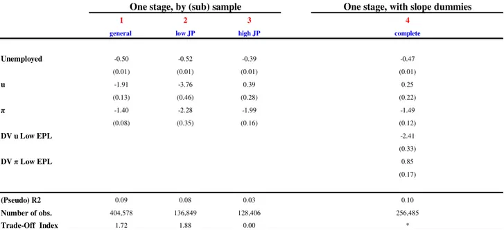
Unemployed -0.50 -0.52 -0.39 -0.47 (0.01) (0.01) (0.01) (0.01) u -1.91 -3.76 0.39 0.25 (0.13) (0.46) (0.28) (0.22) -1.40 -2.28 -1.99 -1.49 (0.08) (0.35) (0.16) (0.12) DV u Low EPL -2.41 (0.33) DV Low EPL 0.85 (0.17) (Pseudo) R2 0.09 0.08 0.03 0.10 Number of obs. 404,578 136,849 128,406 256,485 Trade-Off Index 1.72 1.88 0.00 *
One stage, by (sub) sample One stage, with slope dummies
Table 4.2: One Stage Life-Satisfaction Equations, by JP Sub-Groups
Legend: results from multinomial ordered-probit regressions. Standard errors are in parentheses.
Inflation and unemployment rates are three-year moving averages. All regressions include country and year dummies (France and 1975 are the base), time trend, GDP per capita (in 2000 constant US$) and personal characteristics.
• The Trade-Off Index is reported in Table 6. ** Unemployment is not significant in the
estimate
The difference between costs of unemployment in high and low job protection countries is striking (Table 4.2). The coefficient of the overall level of unemployment (column 3) is not significant in high job protection countries and has a magnitude which is ten times lower than in low job protection countries (where it is highly significant). This is consistent with our expectations given that in countries with low job protection (and lower power of the employed insiders) working individuals are more afraid of a contagion when the “unemployment disease” spreads.
The effect of the unemployed status is also larger in magnitude in low job protection and significantly different from that of high job protection countries. This raises again the puzzle we tried to solve in section 2.1 and interpreted in the light of differences in long term unemployment, unemployment benefits, family and network solidarity and informal economy between the two subgroups. Finally, the inflation rate has a stronger negative impact in low protection countries.
3.2 Robustness checks II: the unemployment/inflation trade-off with one stage estimates
coefficient magnitudes, cutpoints and average predicted happiness levels, we may evaluate the impact of a one percent reduction in unemployment on the share of respondents declaring themselves very satisfied17. As it is well known, the calculation of the marginal effect of a change in a regressor on the probability of declaring oneself very happy in the ordered probit estimate is obtained with the following formula:
)
(
)
(
)
Pr(
VerySatisf
ied
=
F
S
+
∆
S
−
c
−
F
S
−
c
∆
where F is the cumulative normal distribution, S the predicted average satisfaction level and c the highest cutpoint. In order to obtain the implicit marginal rate of substitution we therefore calculate the change (increase) in inflation which restores the initial situation.
Table 5: Change in the Share of Very Satisfied People due to and u
Unemployment Inflation MRS general -1.04 -0.69 1.51 <29 -0.33 -0.33 1.00 29-42 -0.65 -0.32 2.03 42-64 -0.64 -0.32 2.00 >64 -0.32 -0.32 1.00 low JP -0.67 -0.27 2.48 high JP -0.28 -0.56 0.50
Legend: numbers in the first (second) column represent the change in the share of very satisfied
people due to one percent change in the unemployment (inflation) rate. The third column reports the Marginal Rate of Substitution between and u. It shows the increase in the inflation rate which would keep constant the share of very satisfied people after a one percent reduction in unemployment. Indexes are computed using column 1 (general case) and column 10 (age-subgroups) of Table 4.1 and column 4 (JP (age-subgroups) of Table 4.2.
Following this approach we find that a one percent reduction in the unemployment rate increases the number of very happy people by 0.6 percent in the 29-41 and 42-64 age cohorts while by 0.3 percent only in the below 28 and over 64 cohorts (Table 5, first column). We also observe that the degree of job protection changes significantly the relative impact of inflation and unemployment. In low job protection countries a one percent reduction in unemployment (inflation) determines an increase of around
17 Following Di Tella et al. (2003), since the majority (more than 82%) of respondents declared to be satisfied or very satisfied (satisfaction equal to 3 or 4), it is of interest to analyse the probability
.7 (.3) in the proportion of very happy people while in high protection countries the situation is reversed, with the effects of the same changes in unemployment and inflation being .3 (.6).
Looking at the MRS obtained we can see that in low job protection countries a one percent reduction in unemployment needs to be compensated by a 2.48 percent increase in inflation to maintain constant the share of very happy people. Instead, in high job protection countries, a .5 percent increase in inflation is enough to obtain the same result. When we look at age cohorts we find that the preferences of the two extreme classes coincide exactly with the “one-to-one” assumption of the Misery Index, while the rate of substitution rises to 2 and above for the two central cohorts (Table 5, third column).
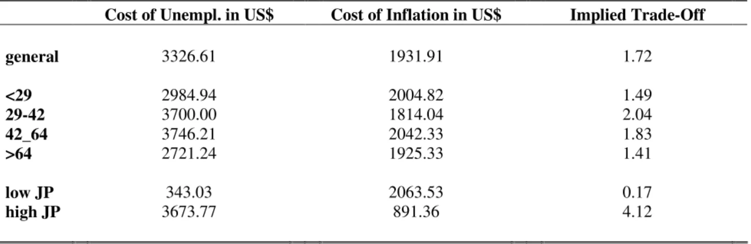
Table 6: Cost of u and
π
in US$ terms and Implied Trade-Off
Cost of Unempl. in US$ Cost of Inflation in US$ Implied Trade-Off
general 3326.61 1931.91 1.72 <29 2984.94 2004.82 1.49 29-42 3700.00 1814.04 2.04 42_64 3746.21 2042.33 1.83 >64 2721.24 1925.33 1.41 low JP 343.03 2063.53 0.17 high JP 3673.77 891.36 4.12
Legend: numbers in the first (second) column represent the amount of US$ necessary to
compensate a one percent increase in the unemployment (inflation) rate. The third column shows the ratio between the cost of a one percent increase in the unemployment rate and the cost of a one percent increase in the inflation rate. Indexes are computed using column 1 (general case) and column 10 (age-subgroups) of Table 4.1 and column 4 (JP subgroups) of Table 4.2.
A second way to obtain the rate of substitution is to consider also the GDP effect on happiness and extract the amount of money necessary to compensate an individual for a one percent rise in unemployment or inflation. Using one-stage regressions with slope-dummy variables we obtain the results shown in Table 6. The cost of a 1% unemployment rate for an individual in low job protection countries is 3,673 dollars against 343 dollars in high job protection countries. Implied trade-offs are markedly different between the low and high job protection subgroups.
When we look at age classes the 42-64 age cohort has the maximum compensation (3,746 dollars), while the over 64 cohort has the minimum one (2,721 dollars). Again, central age cohorts and low job protection countries exhibit extremely high rates of substitution.
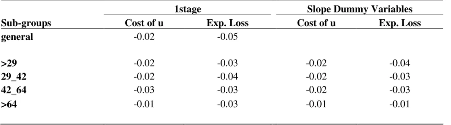
Finally, we repeat the exercise of the implicit rates of substitutions when the cost of unemployment is computed in terms of expected loss for the one stage estimates as well (Table 7) under the two different approaches of class specific estimates and slope dummies in an overall sample regression. The obtained results are in line with previous conclusions.
Table 7: Expected Losses, One-stage Equations
1stage Slope Dummy Variables
Sub-groups Cost of u Exp. Loss Cost of u Exp. Loss
general -0.02 -0.05
>29 -0.02 -0.03 -0.02 -0.04
29_42 -0.02 -0.04 -0.02 -0.03
42_64 -0.03 -0.03 -0.02 -0.03
>64 -0.01 -0.03 -0.01 -0.01
Legend: statistics reported are computed using results of one-stage estimates with and without age
slope-dummies.
4. Robustness checks on the interaction between age cohort and job protection effects
In this section we test whether our separate findings on age cohort and job protection effects persist when the two variables affecting costs of inflation and costs of unemployment are jointly estimated. In doing so, we follow three different approaches. Under the first we run four separate regressions by age groups where participation to the two (low and high) job protection groups is introduced as a dummy variable. Under the second we run a single overall sample regression with separate age and job protection dummies. Under the third, age and job protection dummies in the single overall sample regression are interacted.
Results obtained with the three different methodologies present some important regularities (Table 8). First, the unemployment effect across age cohorts is hump-shaped irrespective of the methodology and the job protection class considered. The central (29-41 and 42-64) classes always have a negative coefficient which is higher in magnitude than in extreme classes. As in our previous findings, it is not clear which one of them has the highest Trade-Off Index, while it is confirmed that the two central classes suffer more than the extreme ones.
high protection ones. These two findings confirm that the effects of age and job protection on the cost of unemployment are remarkably stable and independent from each other.
On the basis of these economic results, we explore how changes in inflation and unemployment influence the share of very happy people using single regression estimates where age and job protection effects are both present (Table 9, first four columns). Again, middle age cohorts and low protected countries present the highest cost of unemployment in terms of “very-happy” people. The strongest impact of a one percent increase in unemployment is the reduction by around 1% in the share of very happy people in the 42-64 age class living in low job protection countries.
Table 8: Life-Satisfaction Equations, Robustness Checks Beta Coefficients and Trade-Off Indexes
Unemployment Inflation Trade-Off Index
Methodology 1 Age Group low JP high JP Age Group low JP high JP Age Group low JP high JP
Four separate <29 -1.93 -1.32 <29 -1.08 -2.44 <29 2.24 0.74 Regressions run 29-41 -2.60 -1.97 29-41 -1.31 -2.44 29-41 2.38 1.02 by Age Groups, with JP 42-64 -2.80 -2.60 42-64 -0.80 -1.62 42-64 3.48 1.91 Slope Dummy Variables >64 -1.03 -0.98 >64 -0.45 -0.94 >64 2.85 1.30
Methodology 2 Age Group low JP high JP Age Group low JP high JP Age Group low JP high JP
One Single Regression <29 -1.93 -1.57 <29 -0.95 -1.82 <29 2.56 1.13 with JP and Age Slope 29-41 -2.40 -2.04 29-41 -0.80 -1.68 29-41 2.23 0.85 Dummy Variables 42-64 -2.44 -2.08 42-64 -0.95* -1.83* 42-64 1.60 1.41
>64 -1.73 -1.37 >64 -0.93* -1.80* >64 1.25 1.03
Methodology 3 Age Group low JP high JP Age Group low JP high JP Age Group low JP high JP
One Single Regression <29 -2.94 -0.11 <29 -0.97 -1.84 <29 3.55 0.32 run with JP and Age 29-41 -2.87* -0.49 29-41 -0.87 -1.78 29-41 3.84 0.55 interacting Slope 42-64 -2.44 -0.77 42-64 -0.72* -1.84 42-64 4.07 0.69 Dummy Variables >64 -1.24 -0.45 >64 0.01 -2.05 >64 ** 0.46
Legend: Reported betas are given by the sum of the coefficients of the base and the slope dummy variable.
* Dummy Variable Not Significant at the 10 percent Level.
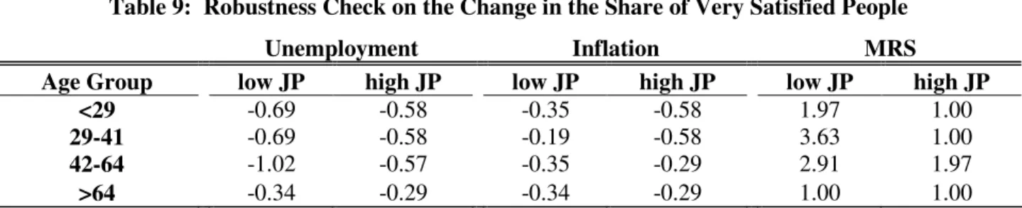
Table 9: Robustness Check on the Change in the Share of Very Satisfied People
Unemployment Inflation MRS
Age Group low JP high JP low JP high JP low JP high JP
<29 -0.69 -0.58 -0.35 -0.58 1.97 1.00
29-41 -0.69 -0.58 -0.19 -0.58 3.63 1.00
42-64 -1.02 -0.57 -0.35 -0.29 2.91 1.97
>64 -0.34 -0.29 -0.34 -0.29 1.00 1.00
Legend: Results are from one-stage regression run with JP and age interacting slope-dummy
variables.
Finally, we calculate the implied marginal rate of substitutions (MRSs) which maintain constant the share of very happy people on the basis of the coefficients just computed (Table 9, fifth and sixth columns). The 29-41 age class in the low job protection countries displays the highest MRS: a one percent reduction in the unemployment rate may be traded off with an increase of 3.63 percent in inflation. All age classes in high job protection countries (with the exception of the 42-64 age class) and the over 64 age class in low job protection countries have low rate of substitutions. The trade-off of all these sub-samples is exactly one and coincides with that implied by the Misery Index.
5. Age, employment protection and economic policies
In the debate on monetary policy strategies economists often contrast the Fed and the ECB for their different attitudes toward price stability and discretion. While the Federal Reserve Act18 gives the same importance to price stability and employment, the European Central Bank Statute19 clearly defines low inflation as the fundamental priority of the Bank20.
18 Federal Reserve Act (1913), Section 2A - Monetary Policy Objectives: “The Board of Governors of the Federal Reserve System and the Federal Open Market Committee shall maintain long run growth of the monetary and credit aggregates commensurate with the economy's long run potential to increase production, so as to promote effectively the goals of maximum employment, stable prices, and moderate long-term interest rates.”
19 Protocol on the Statute of the European System of Central Banks and of European Central
Bank. Objectives and tasks of the ECB (1992). Article 2: “In accordance with Article 105(1) of
this Treaty, the primary objective of the ESCB shall be to maintain price stability. Without prejudice to the objective of price stability, it shall support the general economic policies in the Community with a view to contributing to the achievement of the objectives of the Community as laid down in Article 2 of this Treaty. The ESCB shall act in accordance with the principle of an open market economy with free competition, favouring an efficient allocation of resources, and in compliance with the principles set out in Article 4 of this Treaty.”
20 Since 2003, the ECB adopts the following definition of price stability: inflation is “below but close to 2% over the medium term” (ECB 2003, p. 51). Before 2003, the ECB defined it as a
Several analysts, while praising the Fed’s activism, criticize the “orthodox” approach of the ECB and its “obsession” for price stability. Mishkin (2000) points out that central bankers should not become what Mervyn King (1997) has characterised as “inflation nutters”, but rather care about output as well as inflation fluctuations21. Calling for a greater focus on output growth and employment, some economists compare the Fed’s ability to support real growth with the “sluggish” Bundesbank approach, now inherited by the ECB (see Bibow, 2005). Although it seems rather simplistic to argue that the ECB has behaved more cautiously than the Fed (see Sardoni & Wrai, 2005), data on the different economic performance of the two areas seem to support this criticism (Table 10).
Table 10: Population age and JP index in selected countries
Country Avg popul. Age % Popul. over 65 JP index Inflation Unemployment
Germany 42.6 17.8 20 1.41 8.77 Italy 42.2 19.3 23 2.75 10.34 France 39.1 16.5 21 1.56 10.68 EMU 41.2 17.2 17.8 2.40 9.86 United Kingdom 39.3 15.9 2 2.62 6.04 United States 36.5 12.3 1 2.46 5.06
Legend: Average population age is from the CIA World Facts Book (2006). The % of
population over 65 is from the World Bank's WDI (2003). The JP is from the OECD Employment Outlook (1999) and refers to the average situation in the late 1990s. Unemployment and Inflation rates are averages over the period 1995-2004.
Many factors contribute to shape institutions around the world, their statues and priorities and their economic performances. In our opinion, the demographic structure and the level of employment protection might help to explain, among other things, why some central banks have developed a stronger antinflationary
%” could be anything (even a negative inflation rate). Galí and others (2004) see this change of definition as a possible “preparatory move before an eventual increase in the target inflation rate”.
21 On the same wavelenght Krugman (1996) questions the rhetoric of price-stability, which will bring the only result that Europe's unemployment problem, which would have been severe in any case, will be seriously aggravated. Svensson (2003) wonders when the Eurosystem will improve its monetary policy. He strongly believes that the Eurosystem should just adopt the best-practice strategy of flexible inflation targeting getting rid of all the “stubborn” defense of its cautious strategy. Fitoussi and Creel (2002) blame the ECB for being too technocratic arguing that “there is no reason why a technocratic institution like the ECB should be singularly responsible for defining what 'price stability' means for Europe. Monetary policy is not a purely
stance than others. In Table 10 we can see that the European countries which contributed the most in shaping the ECB and its policies (and which are characterised by older population and higher employment protection) displayed lower inflation and higher unemployment rates over the period 1995-2004.
The United Kingdom, with its lower population age but especially its very low JP index, presents a much lower unemployment rate and a slightly higher inflation than in average EMU countries. A stronger fear of unemployment may have played some role in the British authorities’ decision of not taking part to the MU22. Finally, the United States are characterised by much lower population age, a lower share of over 65 with respect to EMU countries and by an JP index close to zero. If our results hold true even for countries outside the considered sample, and taking into account that the lobbying power of the elderly is notoriously bigger23, we may infer that the higher concern for real outcomes in the US could partly be explained by the different pressures lobbies exert on policy makers. Finally, it is reasonable to think that developing countries, which have a very low share of over 65 and usually low levels of job protection, may be more concerned with promoting economic growth at the expense of a possible higher inflation24.
The traditional macroeconomic view considers people’s preferences as given and largely independent of time and of institutional evolution (see Darity and
22 Gordon Brown, as Chancellor of the Exchequer, in 1997 set out five economic tests on which any decision about UK membership of the EMU should be based:
1. Cyclical convergence: are business cycles and economic structures compatible so that we
and others could live comfortably with euro interest rates on a permanent basis? 2. Flexibility: if problems emerge is there sufficient flexibility to deal with them?
3. Investment: would joining EMU create better conditions for firms making longterm
decisions to invest in Britain?
4. Financial services: what impact would entry into EMU have on the competitive position
of the UK's financial services industry, particularly the City's wholesale markets?
5. Employment and growth: in summary, will joining EMU promote higher growth,
stability and a lasting increase in jobs?
The Executive HM Treasury Report (1997) concluded as follows: “We need to demonstrate sustainable and durable convergence before we can be sure that British membership of EMU would be good for growth and jobs. Joining before such convergence is secured would risk harming both”.
23 For theoretical contributions on the effect of lobbies on economic policy decision see Posen (1995) and Piga (2005). The elderly have more leisure time, they are more stick to their own interests and have a greater ability to organize their fights. “The elderly are politically powerful because they are more single-minded. That is, while young citizens disperse their political capital among many issues, the old tend to vote with very few things in mind” (Mulligan and Sala-i-Martin, 2003).
24 For example, Brazil and India’s shares of over 65 are respectively 5.9% and 5.1%. Reducing the Indian unemployment rate by 1% would mean providing four or five million people with a
Goldsmith, 1996). In the light of our empirical findings it seems legitimate to question this assumption. Preferences are strongly influenced by demographic and institutional variables which, for example, can affect the individual costs of inflation and unemployment. Anyway, it is important to stress that policymakers can act on preferences by affecting a country’s demographic structure and its institutional setting25.
6. Conclusions
Policymakers should not forget that voters’ relative preferences over inflation and unemployment are sharply heterogeneous across age cohorts and are endogenous with respect to changes in the institutional setting, especially if we consider job market regulation.
Furthermore, authorities should consider that, when it comes to inflation and unemployment, two radically different things are compared. On the one side we have an “illness” which affects directly only some individuals (unemployment) but engenders fear of contagion in many others. On the other side we have a pervasive environmental factor which affects everyone (even though individuals may have different capacity of insulation from it).
In this perspective, age and job protection are two fundamental variables explaining the heterogeneity of the individuals’ relative preferences between inflation and unemployment, since “probabilities of contagion” from the “unemployment illness” for those actually employed are markedly different when the two above mentioned factors vary.
Following this intuition we demonstrate in the paper that the negative effect of unemployment on individual happiness is much lower for those individuals who, for age class and institutional framework, are less likely to be affected by such illness (or have relatively reduced consequences from the infection). This implies that an average marginal rate of substitution between unemployment and inflation, calculated on the entire sample population (1.91 with a 91 percent higher weight on unemployment) hides dramatically different rates of substitutions according to different age cohorts and domestic job market rules.
Such heterogeneity may push the index well above two for low job protection countries and to one and below for high job protection ones. This may help to understand how some economic institutions have been shaped and behave. We have in mind, for instance, the stronger pro-employment stance of US versus EU central bankers, the decision of a low job protection country such as the UK of not
entering the MU and the relatively milder attitude of core EU economies (with an aging population and high job protection) toward a concerted fight against unemployment.
References
[1] Akerlof, G., Dickens, W. and Perry, G. (1996). “The Macroeconomics of Low Inflation” [including comments by Gordon and Mankiw]. Brookings Papers on Economic Activity, 1996(1):1-59 [60-76].
[2] Alesina, A., Di Tella, R. and MacCulloch, R. (2004). “Happiness and Inequality: Are Europeans and Americans different?”. Journal of Public Economics, Vol. 88, pp. 2009-2042.
[3] Barro, R. and Gordon, D. (1983). “ Rules Discretion and Reputation in a Model of Monetary Policy”. Journal of Monetary Economics, 12, pp.101-121.
[4] Bibow, J. (2005). “Refocusing the ECB on Output Stabilization and Growth through Inflation Targeting?”. Working Paper 425. Annandale-on-Hudson, N.Y.: The Levy Economics Institute.
[5] Blanchflower, D. (1996). “Youth Labor Markets in Twenty Three Countries: A Comparison Using Micro Data”. In: David Stern (eds). School to Work Policies and Practices in Thirteen Countries. Cresskill: Hampton Press.
[6] Brown, G. (1997), “Speech to the Royal Institute for International Affairs”, www.hm-treasury.gov.uk, HMSO, London.
[7] Clark, A., Georgellis, Y. and Sanfis, P. (2001), “Scarring: The Psychological Impact of Past Unemployment”. Economica, 68:270, pp.221-41.
[8] Clark, A. and Oswald, A. (1994). “Unhappiness and Unemployment”. Economic Journal, Vol. 104, pp. 648-659.
[9] Darity, W. and Goldsmith, A. (1996). “Social Psychology, Unemployment and Macroeconomics”. Journal of Economic Perspectives, Vol. 10(1), pp. 121-140.
[10] De Grauwe, P. (2005). “Economics of Monetary Union”. 6/e.Oxford: Oxford University Press.
[11] Di Tella, R. and MacCulloch, R. (2003). “The Macroeconomics of Happiness”, Review of Economics and Statistics. November 2003, 85(4): 809–827, MIT Press.
[12] Di Tella, R., MacCulloch, R. and Oswald, A. (2001). “Preferences over Inflation and Unemployment: Evidence from Surveys of Happiness” . American Economic Review, 91(1): 335-341.
[13] Dickens, W. (2001). “Comments on Charles Wyplosz Paper: Do We Know How Low Should Inflation Be?”. In Why Price Stability? First ECB Central Banking Conference. Frankfurt am Main: European Central Bank.
[14] Dusenberry, J. (1949). “Income, Saving and Theory of Consumer Behavior”. Harvard University Press, Cambridge.
[15] European Central Bank (2003). “The ECB’s Monetary Policy Strategy,” Press Release, 8th of May 2003, www.ecb.int .
[16] European System of Central Banks (1992). Protocol on the Statute of the European System of Central Banks and of European Central Bank. Objectives and tasks of the ECB. www.ecb.int .
[17] Feather, N. (1990). “The Psychological Impact of Unemployment”. New York: Springer.
[18] Federal Reserve Act (1913), as amended by acts of 1978, 1988 and 2000. www.federalreserve.gov .
[19] Fitoussi, J.P. and Creel, J. (2002). “How to Reform the European Central Bank” , New CER Pamphlet. www.cer.org .
[20] Frey, B. and Stutzer, A. (2000). "Happiness, Economy and Institutions". Economic Journal, Vol. 110, pp. 918-938.
[21] Frey, B. and Stutzer, A. (2002). “What can Economists learn from Happiness Research”. Journal of Economic Literature, Vol. 40, pp. 402-435.
[22] Friedman, B. (2004). “Why the Federal Reserve Should Not Adopt Inflation Targeting.” International Finance, Vol. 7 (1), pp. 129-136.
[23] Galí, J., Gerlach, S., Rotemberg, J., Uhlig, H., and Woodford, M. (2004). “The Monetary Policy Strategy of the ECB Reconsidered: Monitoring the European Central Bank 5”, London: Centre for Economic Policy Research.
[24] Hirsch, F. (1976). “Social Limits of Growth”. Harvard University Press, Cambridge, Massachusetts.
[25] HM Treasury (1997). “Uk Membership of a Single Currency: An Assessment of the Five Economic Tests”. www.hm-treasury.gov.uk, HMSO, London.
[26] King, M. (1997). “Changes in U.K. Monetary Policy: Rules and Discretion in Practice”. Journal of Monetary Economics, Vol. 39 (1), pp. 81-97.
[27] Krugman, P. (1996). “Stable Prices and Fast Growth: Just Say No”. The Economist, 31st of August 1996.
[28] Malthus, T. (1798). “An Essay on the Principles of Population”. Published for J. Johnson, London.
[29] Marshall, A. (1890). “Principles of Economics”. MacMillan, London, 1947.
[30] Mishkin, F. (2000). ”What Should Central Banks Do”, Federal Reserve Bank of St. Louis Review, November/December, pp. 1-14.
[31] Mulligan, C. and Sala-i-Martin, X. (1999). “Gerontocracy, Retirement and Social Security”. NBER Working Paper No. 7117.
[32] Nickell, S. (1997). “Unemployment and Labour Market Rigidities: Europe versus North America”. Journal of Economic Perspectives, Vol. 11 (3), pp. 55-74.
[33] Nickell, S., Nunziata, L. and Ochel, W. (2005). “Unemployment in the OECD Since the 1960’s. What Do We Know?" The Economic Journal , Vol. 115 (January), pp. 1–27.
[35] Piga, G. (2005). “On the Sources of the Inflation Bias and Output Variability” Scottish Journal of Political Economy, Vol. 52(4), pp. 607-622. [36] Posen, A. (1995). "Declarations Are Not Enough: Financial Sector Sources
of Central BankIndependence", NBER Macroeconomic Annual, pp. 253-274.
[37] Rich, G. (2005). “European Monetary Policy: Can the ECB learn from the Fed?”. www.richcons.ch , University of Bern, Mimeo.
[38] Rogoff, K. (1985). “The Optimal Commitment to an Intermediate Monetary Target”. Quarterly Journal of Economics, Vol. 100, pp. 1169-1189.
[39] Sardoni, C. and Wrai, R. (2005). “Monetary Policy Strategies of the European Central Bank and the Federal Reserve Bank of the U.S.”. Working Paper No. 431, The Levy Economics Institute of Bard College.
[40] Svensson, L. E. O. (2003). “How should the Eurosystem Reform Its Monetary Strategy”, Briefing paper for the quarterly testimony of the President of the European Central Bank before the Committee on Economic and Monetary Affairs of the European Parliament.
[41] Veblen, T. (1899). “The Theory of the Leisure Class”. Dover Publications, New York.
[42] Winkelmann, L. and Winkelmann R. (1998). “Why Are the Unemployed So Unhappy? Evidence from Panel Data”. Economica, Vol. 65 (257), pp. 1-15.
[43] Wyplosz, C. (2001). “Do We Know How Low Should Inflation Be?”. CEPR Discussion Paper No. 2722.
Appendix
Table A1: 1st stage of two-stage estimation, General & JP Sub-Groups
general Low JP High JP
unemployed -0.34 (0.00) -0.35 (0.01) -0.29 (0.01) selfemployed 0.05 (0.01) 0.05 (0.01) 0.06 (0.02) male -0.04 (0.00) -0.07 (0.00) -0.01 (0.00) age -0.02 (0.00) -0.02 (0.00) -0.02 (0.00) age2 0.00 (0.00) 0.00 (0.00) 0.00 (0.00) mideduc 0.04 (0.00) 0.04 (0.01) 0.06 (0.01) higheduc 0.08 (0.00) 0.09 (0.01) 0.11 (0.01) married 0.07 (0.00) 0.08 (0.01) 0.10 (0.01) divorced -0.15 (0.01) -0.15 (0.01) -0.13 (0.02) separated -0.20 (0.01) -0.22 (0.02) -0.15 (0.02) widowed -0.09 (0.01) -0.09 (0.01) -0.10 (0.01) income_2q 0.14 (0.00) 0.11 (0.01) 0.16 (0.01) income_3q 0.24 (0.00) 0.22 (0.01) 0.26 (0.01) income_4q 0.32 (0.00) 0.31 (0.01) 0.32 (0.01) retired 0.01 (0.00) 0.00 (0.01) 0.04 (0.01) student 0.14 (0.02) 0.13 (0.03) 0.13 (0.04) R-squared 0.18 0.14 0.07 Number of obs 409,079 128,406 128,406
Legend: These are the results from a first-stage OLS regression. Standard errors are in
parenthesis. Regressions include country and year dummies. Variables are defined in Table 1.