Master of Science in Computer Engineering School of Industrial and Information Engineering
A Plenacoustic Approach
to Sound Scene Manipulation
Master Graduation Thesis of: Francesco Picetti
Candidate Id: 855153
Supervisor:
Prof. Fabio Antonacci Assistant Supervisor: Dr. Eng. Federico Borra
Corso di Laurea Specialistica in Ingegneria Informatica Scuola di Ingegneria Industriale e dell’Informazione
Un Approccio Plenacustico
alla Manipolazione di Scene Sonore
Tesi di Laurea Specialistica di:: Francesco Picetti
Matricola: 855153
Relatore:
Prof. Fabio Antonacci Correlatore:
Dott. Ing. Federico Borra
Sound field manipulation is a research topic that aims at modifying the properties of an acoustic scene. In the literature it has been proven that physically accurate sound field representations become unpractical when complex sound scenes are considered, due to the enormous computational effort they would require.
This thesis aims at developing a novel manipulation methodology based upon Soundfield Imaging techniques, which model the acoustic propagation adopting the concept of acoustic rays, i.e. straight lines that carry acoustic information. We have taken advantage of the Ray Space
Transform, a powerful tool that efficiently maps the sound field
informa-tion acquired by means of a Uniform Linear Array (ULA) of microphones onto a domain known as ray space. Points in this domain represent rays in the geometric space, therefore the analysis of the propagating sound field could be addressed considering each directional component individ-ually.
The description of acoustic scenes is here approached adopting a para-metric spatial sound paradigm. More precisely, the sound scene is de-scribed by defining the acoustic source, its position and orientation in space, its emitted signal and finally its radiation pattern, defined as the angular-frequency dependence of the amplitude of the signal.
First, the ray space transform of the microphone signals is computed and provided to the parameter estimation stage. In particular, the source position is estimated through a weighted least squares problem, while the radiation pattern is extrapolated from the linear pattern of the ray space image. Since the microphone array "sees" the source from a narrow range of directions, the radiation pattern is modelled in the Circular
Harmon-ics domain and the coefficients are estimated through an optimization
problem. Finally, a spatial filter called beamformer is designed upon the results of the previous steps in order to extract the source signal directly from the array signals.
The estimated paramaters could be provided to any parametric sound scene rendering system. Through computer-aided simulations and exper-iments we have proven the capability of the proposed system performing different manipulations. The results of the tests suggest that the pro-posed methodology would play a significant role in future research topics on spatial audio processing.
La manipolazione dei campi acustici è un argomento di ricerca che si prefigge di modificare le proprietà di una scena acustica. In letteratura è stato comprovato che le rappresentazioni fisicamente accurate del campo sonoro risultano impraticabili nella modellazione di scene complesse, a causa dell’ingente costo computazionale richiesto.
Questa tesi sviluppa una metodologia di manipolazione innovativa basata sulle tecniche di Soundfield Imaging, nelle quali la propagazione sonora sfrutta il concetto di raggi acustici, ovvero linee rette che traspor-tano informazione acustica. Abbiamo adottato la trasformata Ray Space, un potente operatore che mappa l’informazione acquisita da una schiera lineare uniforme di microfoni nello spazio dei raggi. Punti in questo do-minio rappresentano raggi nello spazio geometrico, perciò l’analisi della propagazione del campo acustico può essere affrontata considerando in-dividualmente le componenti direzionali.
La descrizione della scena acustica fa proprio il paradigma parame-trico della spazializzazione sonora. Più precisamente, la scena acustica è qui parametrizzata definendo la sorgente acustica, la sua posizione e il suo orientamento nello spazio, il suo segnale emesso e infine il pattern di radianza, definito come la dipendenza dell’ampiezza del segnale dalla frequenza e dalla direzione di propagazione.
Innanzitutto i segnali microfonici viengono trasformati e l’immagine ray space processata per stimare i parametri. In particolare, la posizione della sorgente è stimata grazie a una regressione ponderata dei minimi quadrati, mentre il pattern di radianza è estrapolato dalla linea emer-gente dall’immagine ray space. Siccome la schiera di microfoni "vede" la sorgente in un intervallo ristretto di direzioni, il pattern di radianza è modellato nel dominio delle Armoniche Circolari e i coefficienti stimati con un problema di ottimizzazione. Infine, un filtro spaziale chiamato
beamformer viene progettato conoscendo i risultati dei passaggi
prece-denti al fine di estrarre il segnale della sorgente direttamente dai segnali microfonici.
I parametri stimati possono essere utilizzati da qualsiasi sistema pa-rametrico di rendering acustico. Grazie a simulazioni computerizzate ed esperimenti in laboratorio abbiamo dimostrato le capacità del sistema proposto eseguendo diverse manipolazioni. I risultati delle prove sugge-riscono che la metodologia proposta giocherà un ruolo importante nelle ricerche future sull’elaborazione di campi acustici.
Questa tesi è stata sviluppata presso l’Image and Sound Processing Lab del Politecnico di Milano ed è il risultato di un lungo percorso accademico. Vorrei innanzitutto ringraziare il mio relatore, prof. Fabio Antonacci, per avermi dato l’opportunità di lavorare ad un argomento così interes-sante. Un rigraziamento speciale merita il mio correlatore, Federico, per l’inestimabile pazienza e il prezioso supporto offertomi nei momenti più difficili di questo lavoro.
La mia gratitudine va anche ai miei compagni di corso e a tutto il gruppo ISPL-ANTLAB. Ricorderò particolarmente Clara, Stella, Jacopo e Luca; grazie per gli incoraggiamenti e l’affetto, per le discussioni sui grandi sistemi e sui piccoli sintetizzatori.
Grazie alla mia famiglia, ai miei genitori e ai miei fratelli, per l’immenso supporto e sostegno. Non avrei raggiunto questo traguardo senza di voi. Infine una dedica speciale va ad Alice, che rende la vita migliore.
F.P.
Dimenticavo. Grazie a Wolfgang che dà un senso a tutto questo. Anche se è morto.
Abstract i
Sommario ii
Ringraziamenti iii
List of Figures vi
List of Tables vii
Introduction viii
1 State of the Art 1
1.1 Acoustic Field Representation . . . 2
1.1.1 Plane Waves Decomposition . . . 3
1.1.2 Green Function . . . 3
1.1.3 Kirchhoff-Helmholtz Integral . . . 4
1.2 Sound Field Synthesis Methodologies . . . 5
1.2.1 Stereophony . . . 6
1.2.2 Ambisonics . . . 7
1.2.3 Wave Field Synthesis . . . 8
1.3 Ray Acoustics . . . 9
1.3.1 The Eikonal Equation . . . 10
1.3.2 Spatial Filtering: the Beamformer . . . 11
1.4 Plenacoustic Imaging . . . 14
1.4.1 The Reduced Euclidean Ray Space . . . 15
1.5 Conclusive Remarks . . . 17
2 Theoretical Background 18 2.1 Ray Space Transform . . . 19
2.1.1 Remarks . . . 22
2.1.2 Source Localization in the Ray Space . . . 22
2.2 Radiation Pattern . . . 23
2.2.1 Definition . . . 24
2.2.2 Circular Harmonics Decomposition . . . 24
2.2.3 Radiation Pattern and Soundfield Imaging . . . . 25
2.2.4 Remarks . . . 25
3 Acoustic Scene Analysis and Manipulation 27
3.1 Scene Analysis . . . 28
3.1.1 Source Localization . . . 30
3.1.2 Orientation and Radiation Pattern Extraction . . 30
3.1.3 Signal Extraction . . . 34
3.2 Scene Synthesis . . . 36
3.2.1 Geometry Synthesis . . . 36
3.2.2 Radiation Pattern Synthesis . . . 36
3.2.3 Signal Synthesis . . . 37
3.3 Conclusive Remarks . . . 38
4 Simulations and Tests 39 4.1 Evaluation Metrics . . . 39 4.2 Simulations . . . 40 4.2.1 Scene Analysis . . . 42 4.2.2 Scene Synthesis . . . 42 4.3 Experiments . . . 45 4.3.1 Scene Analysis . . . 46 4.3.2 Scene Synthesis . . . 47 4.4 Conclusive Remarks . . . 49
5 Conclusions and Future Works 50 5.1 Future Works . . . 51
Appendices - Equipment Specifications 53 A Beyerdynamic MM1 . . . 53
B Focusrite Octopre LE . . . 55
1 An example of acoustic scene and manipulation. . . x
1.1 Geometry of a boundary value problem in 2D. . . 5
1.2 The most common configuration for 2-channels stereophony. 6 1.3 The Huygens principle (courtesy of [1]). . . 9
1.4 Uniform Line Array (ULA). . . 11
1.5 Ray Space representation of a point source in r′. . . 16
2.1 (m, q) line (in red) and magnitude of the RST for an isotropic point source, emitting a pure tone at 2 kHz, placed in r′ = [1, 0] m. . . . 21
3.1 Block diagram for the whole manipulation system. . . 28
3.2 The ULA and the coordinate systems of the audio scene. 29 3.3 Block diagram of the localization. . . 30
3.4 Block diagram of the radiation pattern extraction. . . 31
3.5 Block diagram of the signal extraction. . . 35
3.6 The acoustic curtain paradigm. . . 37
4.1 The simulated scene geometry. . . 41
4.2 The localization error (left) and the orientation error (right) for the simulated scene. . . 43
4.3 NMSE values when manipulating the source orientation. 44 4.4 NMSE values (right) when manipulating the angular co-ordinate (left). . . 44
4.5 NMSE values (right) when moving the source away (left). 45 4.6 NMSE values (right) when moving the source towards the array (left). . . 45
4.7 The loudspeaker and the microphone array in the experi-mental setup. . . 46
4.8 NMSE values when manipulating the source orientation. 47 4.9 NMSE values (right) when manipulating the angular co-ordinate (left). . . 48
4.10 NMSE values (right) when moving the source away (left). 48 4.11 NMSE values (right) when moving the source towards the array (left). . . 49
4.1 Ray Space Transform parameters. . . 41
4.2 STFT parameters. . . 42
4.3 The audio equipment of the experiment. . . 46
Processing of sound field is a research topic that aims at manipulating the sound field in order to extract information about the overall acoustic characteristics of both the environment and the objects in a scene. The ability to sense spatial properties of sound enables humans to experience immersivity, i.e the sense of presence in a scene. In the last decades this topic has grown interest in both research and industry communities, since it can be applied to a great variety of markets and purposes. As an example, in multimedia and entertainment industry we would cite live music venues, movie theatres, videogames, and teleconference. Moreover, this topic is experiencing a growth in interest also in sound and vibration control, e.g. in the automotive industry.
This thesis addresses the problem of manipulating a sound scene and proposes a novel synthesis-by-analysis methodology based on geometrical acoustics. In order to capture the spatial cues of the sound propagation, a suitable field representation is needed. Among all the acoustic field rep-resentations, we can distinguish between two main paradimgs. The so called nonparametric representations describe the acoustic field as a func-tion of space and time and assume no a-priori knowledge on the acous-tic scene. These physically-motivated reprepresentations decompose the sound field on different basis functions. We would cite Ambisonics and its followers, which decompose the sound field in terms of spherical har-monics, and WaveField Synthesis that is based on the Huygens’ principle, which states that the wavefront of a primary source can be reconstructed through a conveniently-driven spatial distribution of secondary sources, e.g. loudspeakers. Although their physical motivation and precision, the nonparametric representations require an enormous computational effort in order to solve exactly the wave equation and its boundary conditions, especially in modelling complex acoustic environments.
The second paradigm is the geometric representation and it models the acoustic propagation upon the concept of acoustic rays, i.e. straight lines that carry acoustic information. Although this view provides a rough approximation of an acoustic field, in literature it has been demon-strated that this approach can model complex acoustic environments, for which a physically accurate modelling is not practical. This is the aim of Plenacoustic Imaging [2], a novel technique that maps plane-wave components of the acoustic field to points in the ray space, defined as
a projective domain whose primitives are acoustic rays. If we want to measure the plenacoustic function in a given point, we can do so by using a microphone array centred in that point, and estimating the radiance along all visible directions through spatial filtering. By subdividing the array into small sub-arrays the plenacoustic function can be acquired over every point belonging to the microphone array boundaries. It has been proven [3] that the main acoustic primitives (such as sources and reflec-tors) appear in the ray space as linear patterns, thus enabling the use of fast techniques from computational geometry to deal with a wide range of problems, such as localization of multiple sources and environment inference. One step beyond, in [4] the authors devise a linear operator called Ray Space Transform that maps the signals acquired from a Uni-form Linear Array (ULA) of microphones in the ray space domain. This transformation is based on a short space-time Fourier transform using Gabor frames, enabling the definition of analysis and synthesis operators that exhibit perfect reconstruction capabilities. In other words, the array is subdivided into shifted and modulated replica of a prototype spatial window. Then, for each sub-array, a spatial filter called beamformer scans all the visible directions and encodes the sound field. For the purpose of this thesis, the geometrical acoustics can give us a incisive advantage, because by capturing each ray in a single position in space, the acoustic scenario can be easily reconstructed also in near-field conditions.
In its simplest formulation, a sound scene is described as a source emitting acoustic signals in space. Through a ULA of microphones, the analysis stage aims at localizing the source in space and extracting its sig-nal. Figure1help visualizing the scene and the transformation we aim at applying to it. The manipulation can be described as a three-steps pro-cess. First, the microphone array signal is transformed in the ray space; the localization process can be easily performed trough a weighted least squares regression on the peaks that emerge from the ray space image. Second, the ray space image is read along the linear pattern that is dual of the source position in the geometric space. However, we cannot as-sume the source signal propagation to be constant over the directions. Due to the physical characteristics of the source, the sound propaga-tion prefers some direcpropaga-tions among others. Morever, these inequalities in sound propagation depends on the time frequency; indeed, the acous-tic absorption of the source body depends on the frequency. In order to model these phenomena we adopt the concept of Radiation Pattern as an angular-frequency dependence of the amplitude of the signal emitted (or received) by any acoustic object. The radiation pattern can also describe the orientation of the source in the space; by rotating the radiation pat-tern we can rotate the source about its axes. The ray space components extracted in the second step is thus interpreted as the source
pattern-times-signal. In order to extrapolate the radiation pattern weights that
mask the pure signal, we adopt the Circular Harmonics Decomposition. The extracted ray space components are compensated for the acoustic
Uniform Linear Array of microphones Radiation Pattern of the source Source
MANIPULATION
Figure 1: An example of acoustic scene and manipulation.
channel and then fed to a linearly constrained quadratic programming problem that estimates a suitable set of coefficients in the Circular Har-monics domain. This way, the radiation pattern of the source seen by the microphone array is reconstructed by a simple matrix multiplication. The third step takes advantage of both the localization and pattern ex-trapolation procedures. In particular, the source signal is extracted from the array signal by a simple beamformer that exploits the acoustic trans-fer function from the source to the microphones position, compensated for the radiation pattern attenuations in the set of directions from the source towards the array.
The sound scene analysis results in the estimate of the position, radi-ation pattern and signal of the acoustic source. These parameters can be easily modified and fed to any parametric sound scene rendering system. In fact, the sound field can be recostructed in any point of the region of interest of the ULA. In order to evaluate the validity of the manipula-tion, we sample the sound field with the same microphone array of the anylisis stage; more precisely, we compare the desired sound field with the synthesized version of the same acoustic scene. The extracted signal is propagated from the desired source position to the microphone array; the synthesized microphones are then weighted for the radiation pattern visible by the array and desiderably oriented. The desired radiation pat-tern weights are computed in the Circular Harmonics domain using the coefficients inherited from the analysis stage.
Through computer-aided simulations and experiments, it emerges that the chosen representation allows the manipulation of the sound scene in a very intuitive fashion. With respect to the state of the art, this work
extends the plenacustic processing of sound fields extrapolating the radi-ation pattern directly from the Ray Space Transform of the microphone array signal, opening to new possibilities of processing the sound scene di-rectly in the ray space. Moreover, the parametric spatial sound paradigm adopted in this thesis is proven to be reliable and intuitive.
This thesis is organized as follows. In Chapter 1 we provide an overview on the nonparametric sound field representation as the theo-retical foundations of the sound field analysis and synthesis techniques present in literature. Then, moving to the realm of geometrical acous-tics, we introduce the reader to the plenacoustic imaging techniques that is the solid root of the methodology devised in this thesis. Chapter 2
addresses the theoretical background of the ray space transform, along with an example of application; moreover, we briefly describe the theory and motivations of the acoustic radiation pattern. Chapter 3 is entirely dedicated to the description of the developed manipulation methodology. More precisely, the chapter starts with a description of the parametric spatial sound paradigm useful for describing any acoustic scene; then the analysis and synthesis steps are presented. In Chapter4we provide some simulations and experiments designed for proving the proposed system capabilities. More precisely, we show the manipulation behavior when the analysed sound scene is rotated and translated during the synthesis stage. Finally in Chapter5we draw the conclusions and outline possible future research directions.
1
State of the Art
This chapter introduces the models suitable for describing the genera-tion and propagagenera-tion of sound. In particular, we describe in detail the theoretical foundations of the techniques developed so far for the pur-pose of this work, i.e. the manipulation of sound scene. The first part reviews the wave equations and their simplest solutions (the plane wave and the Green function) along their characteristics. The second section reviews the two sound reproduction techniques that have emerged in the literature from the ’70s, Ambisonics and, later, WaveField Synthesis. In order to overcome the strict limitations of the classical stereophony, these physically-motivated techniques assumes the wavefield to be a superpo-sition of elementary components, in particular Ambisonics decomposes the soundfield through spherical harmonic functions [5], while WaveField Synthesis exploits the Huygens principle, which states that any wave-front can be decomposed into a superposition of elementary spherical wavefronts emitted by secondary sources [6].
The last sections moves from the realm of wave acoustics to the realm of the geometric acoustics, which introduces a novel signal representation paradigm based on the concept of acoustic ray and briefly describes the advent of the plenacoustic imaging.
In this chapter the sound is described by a scalar function, the acoustic
field, whose domain is the union of time and space regions:
p(r, t), r∈ R3, t∈ R (1.1)
is the general form of an acoustic field, with r and t denoting the spatial coordinates and time, respectively. Since the scenario considered in this work is that of a sound field restricted to a plane, we consider only two spatial coordinates that in Cartesian and polar coordinate systems
are denoted by x = ( x y ) r = ( ρ θ ) (1.2) The polar coordinates are related to Cartesian coordinates by the follow-ing relationships: x = ρ ( cos θ sin θ ) r = ( √ x2+ y2 arctan (y/x) ) (1.3) In the linear regime, i.e. the medium of propagation behaves lin-early, the acoustic field can be described by small-amplitude variations of the pressure; considering a volume without any source, in order to be a valid acoustic field in equation (1.1) must satisfy the homogeneous wave
equation
∇2p(r, t)− 1
c2
∂2p(r, t)
∂t2 = 0 (1.4)
where c denotes the speed of propagation in ms−1 and ∇ is the Laplace operator. In many context it is useful to consider acoustic propagation as a function of space and temporal frequency ω. The sound fields are denoted by p(r, t) = P (r, ω)ejωt, being P (r, ω) =F
t{p(r, t)} the Fourier
Transform with respect to the time variable t. The correspondent equa-tion to the (1.4) in the transformed domain can be obtained as:
Ft { ∇2p(r, t)− 1 c2 ∂2p(r, t) ∂t2 } = 0 (1.5)
eploiting the linearity property and the differentiation property of the Fourier Transform and substituting the definition of P (r, ω) it results
∇2P (r, ω) +(ω
c
)2
P (r, ω) = 0. (1.6)
The equation above is known as Helmholtz equation.
If the volume under consideration is not free of sources, the wave equation loses its validity. In order to include a source excitation term, the right-hand side of (1.4) is replaced with a suitable source term de-pending on the volume flow rate per unit volume q(r, t), yielding the
inhomogeneous wave equation ∇2p(r, t)− 1 c2 ∂2p(r, t) ∂t2 =− ∂q(r, t) ∂t (1.7)
and its related inhomogeneous Helmholtz equation
∇2 P (r, ω) + (ω c )2 P (r, ω) =−jωQ(r, ω). (1.8)
1.1
Acoustic Field Representation
In this section we discuss some mathematical and physical solutions to equation (1.6) in the Cartesian reference frame, without loss of generality, and their main characteristics for analysis and synthesis tasks.
1.1.1
Plane Waves Decomposition
A simple canditate solution to the equation (1.6) is in the form of complex exponential function
P (r, ω) = ej⟨k,r⟩, (1.9)
where k is called the wavenumber vector and the unit vector bk = k/∥k∥ is identified as the Direction of Arrival (DoA) of the plane wave. For sound fields in the form expressed by equation (1.9) to be solutions of the Helmholtz equation, k must be inR2 and satisfy the dispersion relation:
∥k∥2 = (ω c )2 . (1.10)
Upon varying k inR3 constrained by the dispersion relation, one obtains a complete set of basis functions over which an arbitrary acoustic fields may be decomposed. The wave equation (expressed with respect to either time or temporal frequency) is linear, therefore general solutions can be obtained as superposition of plane waves of different frequencies and directions: P (r, ω) = ( 1 2π )3∫∫∫ D ˜ P (k)ej⟨k,r⟩d3r, D = { k∈ R3 :∥k∥ = ω c } . (1.11) In the literature, the expansion in (1.11) is also known as Whittaker’s representation.
1.1.2
Green Function
Arbitrary solutions to the inhomogeneous Helmholtz equation (1.8) are constructed starting from a basic solution, resulting by imposing a spatial impulse at location r′ as the excitation term, i.e.
Q(r, ω) = δ(r− r′)δ(ω),
where δ(·) is the Dirac delta function. The sound field G(r|r′, ω) is
solu-tion to the inhomogeneous Helmholtz equasolu-tion obtained upon substitut-ing the spatial impulse into (1.8):
∇2G(r|r′, ω) +(ω
c
)2
G(r|r′, ω) =−δ(r − r′). (1.12) The function G(·) is called Green function; under free space conditions it takes the form:
G(r|r′, ω) = e
−j(ω/c)∥r−r′∥
4π∥r − r′∥ (1.13)
As for the homogeneous case, general solutions can be obtained by super-position of acoustic monopoles, described by different Green functions.
Finally, we describes the directional gradient of G(r|r′, ω), as an
ex-ample, with respect to r [6]:
∂G(r|r′, ω) ∂r = 1 4π ( jω c − r ρ ) e−jω/cρ ρ2 , (1.14)
ρ being the distance between r and r′, thus ρ = ∥r−r′∥. Equation (1.14) can be interpreted as the spatial transfer function of a dipole source whose main axis is along the r-axis [7].
1.1.3
Kirchhoff-Helmholtz Integral
So far we have considered only the free-field scenario, i.e. where no sound reflections occur. However, there are situations in which one has to consider also the presence of acoustic boundaries. Two of the most important boundary conditions are:
Dirichlet Boundary Condition The boundary constrains a value to the acoustic field itself, i.e. P (r, ω) is constrained for r ∈ ∂S. These boundaries are known as Dirichlet problems and their general formulation is:
P (r, ω) = F (r, ω) ∀r ∈ ∂S (1.15)
Usually the field is forced to vanish for F (r, ω) = 0 ∀r ∈ ∂S, thus it describes a pressure-release boundary.
Neumann Boundary Condition The boundary constrains the normal directional derivative of the acoustic field:
⟨∇P (r, ω), bn(r)⟩ = F (r, ω) ∀r ∈ ∂S (1.16) where ⟨·, ·⟩ denotes the scalar product of two vectors and bn(r) denotes the unit vector normal to ∂S at a point r ∈ ∂S. If the right-hand side of the inhomogeneous Neumann boundary condition is forced to vanish, this condition describes a sound hard boundary (e.g. a perfectly reflective wall).
Kirchhoff-Helmholtz Integral Equation Consider the area S and its boundary ∂S as depicted in figure 1.1. The boundary value problem is ∇2P (r, ω) +(ω c )2 P (r, ω) = F (r, ω), r∈ S (1.17) α⟨∇P (r, ω), bn(r)⟩ + βP (r, ω) = 0, ∀r ∈ ∂S (1.18) where α, β ∈ [0, 1] account the contributions of the different boundary conditions.
S ∂S
ˆ n(r)
r
Figure 1.1: Geometry of a boundary value problem in 2D.
The solution is based on the Huygen’s principle, which states that the wavefront of a propagating wave can be reconstructed by a superposition of spherical waves radiated from every point on the wavefront at a prior instant. Its formulation, the Kirchhoff-Helmholtz integral, takes the form
a(r)P (r, ω) = P0(r, ω)+
I
∂S
(G(r|r′, ω)⟨∇P (r′, ω),bn(r′)⟩ − P (r′, ω)⟨G(r|r′, ω),bn(r′)⟩) dr′ (1.19) where a(r) is a discrimination term:
a(r) = 1 for r∈ S 0.5 for r∈ ∂S 0 for r /∈ S. (1.20)
The equation (1.19) can be interpreted as in figure 1.1. The acoustic field inside the area S is uniquely determined by three contributions:
1. the acoustic field P0(r, ω) due to the source F (r, ω);
2. the acoustic pressure on ∂S;
3. its directional gradient in the direction normal to ∂S.
The Kirchhoff-Helmholtz integral allows the derivation of physically-motivated acoustic field synthesis methodologies that will be presented in section 1.2.3.
1.2
Sound Field Synthesis Methodologies
This section reviews the key-points of the sound reproduction techniques, starting from the conventional stereophony to the best-known method-ologies that receive attention nowadays, Near-field Compensated HigherOrder Ambisonics (NFC-HOA) proposed in [8], and Wave Field
Synthe-sis (WFS) proposed in [9]. The goal of any spatial sound reproduction system is to generate an acoustic field in a way that the listener will perceive the desired sound scene, i.e. he/she will be able to correctly localize all the virtual sources and objects, such as walls.
Figure 1.2: The most common configuration for 2-channels stereophony.
1.2.1
Stereophony
The simplest technique is the two channel stereophony, which exploits both level and time differences between the two loudspeaker signals. Con-sider s(t) as the virtual source signal, the loudspeaker signals are
dL(t) = gLs(t− τL); dR(t) = gRs(t− τR);
(1.21) where gL, gR are the gains for the left and right loudspeakers,
respec-tively, and τL, τR are the time delays for the left and right loudspeakers,
respectively.
Assuming the loudspeakers to be in the far field with respect to the listener position, they can be considered as ideal generators of plane waves (described in (1.9)). The most popular loudspeaker arrangement is depicted in figure1.2; it assumes that the positions of the loudspeakers and that of the listener make up an equiangular triangle. In this setting, the listening position is called sweet spot [6]. For any virtual source whose DoA (Direction of Arrival) θ is between −θ1 and θ1, it holds that
sin θ = sin θ1
1− gL/gR
1 + gL/gR
(1.22) from which one can extract the gain ratio
gL gR
= sin θ1− sin θ sin θ1+ sin θ
. (1.23)
This approximation holds only if the loudspeakers and the listener positions are respected, and it exhibits a pronounced sweet spot. Out-side the optimality, the spatial perception and also timbral balance de-grade. Moreover, the virtual source range is restricted between the two loudspeakers. Indeed, the two loudspeakers act as an angular acoustic window, imposing that θ∈ [−θ1; θ1].
In order to extend the rendering capabilities to all the directions, many other loudspeakers should be added and placed in order to surround the listener, giving birth to the so called uniform circular array. This
is the case of the Vector Based Amplitude Panning (VBAP) technique, which selects the pair of loudspeakers adjacent to the DoA to be rendered and applies to them the gain ratio in equation (1.23).
1.2.2
Ambisonics
The goal of Ambisonics is to extend the panning methods presented above by not using only the loudspeakers closest to the desired source direc-tion. Morover it represents the sound field by a set of signals that are independend on the transducer setup used for recording or reproduction. Ambisonic representation is based on spherical harmonic decomposition of the sound field; in the 2D scenario of interest for the purpose of this work, the pressure field can be written in the cylidrical coordinate system as the Fourier-Bessel series, whose terms are the weighted products of directional functions and radial functions
P (ρ, θ) = B00+1J0(kρ) + ∞ ∑ m=1 √ 2Jm(kρ) ( Bmm+1 cos mθ + Bmm−1 sin mθ), (1.24) where Jm(·) is the Bessel function of order m and Bmmσ is the 2D
am-bisonic component, which can be interpreted as follow: B00+1 is the pres-sure, B11+1 and B11−1 are related to the gradiented (or also the acoustic velocity) with respect to x and y, respectively.
In practice, let us consider an evenly spaced distribution of N loud-speakers, whose positions are rn= R [cos θnsin θn]T with n = 0, . . . , N−
1. The desired sound field, as it woud be generated by the virtual primary sources, is then given as:
P (r, ω) = N∑−1
n=0
DHOA(θn, R, ω)V (r, rn, ω), (1.25)
where DHOA(θn, R, ω) denotes the driving signal for the n-th secondary
source and V (r, rn, ω) = j4H (2) 0 (ω c|r − rn| )
in order to compensate also the near-field instead of using the plane wave assumption of equation (1.11). Finally, the near-field compensated driving functions are:
DHOA(θn, R, ω) = j 4 1 N N′ ∑ ν=−N′ j−νe −jνθP Wejνθn Hν(2) (ω cR ) (1.26)
where ν are the angular frequencies, whose limitation results in a finite series expansion of the plane wave; due to the properties of the Bessel functions, the approximation of the plane wave will be better for low frequencies and smaller distances to origin. For very low orders the wave field will be exact only at the center of the array, limiting the sweet spot. A great variety of optimizations of Ambisonics panning functions has been proposed in literature, e.g. [10], [11].
1.2.3
Wave Field Synthesis
In this subsection we introduce Wave Field Synthesis (WFS) as a phys-ically motivated soundfield reproduction technique. In particular, it is based on the Kirchhoff-Helmholtz integral. Then we illustrate an ap-proach to simplify the implementation of a WFS rendering system adopt-ing only monopole secondary sources easily implemented by loudspeakers on the virtual surface ∂S as stated by the Huygens principle; figure 1.3
helps visualizing this concept. From a technological point of view, dipole sources (modelled by the directional gradient of the Green function) can be implemented by mounting a loudspeaker on a flat panel, thus they are less efficient. Dipole sources are discarded by applying the Neumann boundary condition to the second addend of the integrand in (1.19)
⟨G(r|r′, ω),bn(r′)⟩ = ∂
∂bnG(r|r
′, ω) = 0 r′ ∈ ∂S. (1.27)
The solution is known as Neumann Green function and it satisfies the boundary condition by taking the form
GN(r|r′, ω) = G(r|r′, ω) + G(¯r(r)|r′, ω), (1.28)
where the position ¯r(r) is the mirror image of r with respect to the tangent plane in r′ on the bound ∂S. Moreover, on the boundary we can write
GN(r|r′, ω) = 2G (r|r′, ω) , (1.29)
which can be inserted as Green function into the Kirchhoff-Helmholz integral (1.19): P (r, ω) =− I ∂S 2G(r|r′, ω) ∂ ∂nP (r ′, ω)dr′. (1.30)
The result of equation (1.30) is known as the type-I Rayleigh integral and it describes the sound field inside an area S generated by a distribution of monopole sources placed on the boundary ∂S.
Substituting the Green function in (1.13) in the type-I Rayleigh inte-gral (1.30) leads to
P (r, ω) =−
I
∂S
G0(r|r′, ω)D(r|r′, ω)dr′ r∈ S, (1.31)
where D(r|r′, ω) denotes the monopole source signals D(r|r′, ω) = 2A(ρ)H(ω) ∂
∂nP (r
′, ω). (1.32)
Here, A(ρ) =√2πρ and H(ω) = √jωc are, respectively, a space-dependent attenuation term based on the distance ρ = ∥r − r′∥ and a frequency-dependent term, which are both derived from the far-field Hankel func-tion approximafunc-tion applied to the 2D Green funcfunc-tion:
H0(2) (ω cρ ) ≈ √ 2j π(ωcρ)e −j(ω cρ) (1.33)
Figure 1.3: The Huygens principle (courtesy of [1]). ˜ G(ρ, ω) = H(ω)A(ρ)e −j(ω cρ) 4πρ . (1.34)
In conclusion, WFS reproduction is described as a sampling-interpolation process:
• sampling the continuous driving function at the desired secondary
source positions, and
• interpolation of the driving function into the listening area.
The spectrum of the secondary sources are not band-limited in the an-gular frequency domain (i.e. the direction θ) thus the system will not result in an alias-free reproduction. Moreover, no exact reproduction is achieved for nonlinear/planar systems and sampling artifacts exhibit irregular structures.
1.3
Ray Acoustics
In real acoustic propagation problems it may be impractical to solve the wave equation and its boundaries due to the computational costs that would be required. This is the case of realistic room acoustics.
This section introduces the geometrical acoustic starting from the high frequency approximation of the wave equation, which states that the sound wave travels in straight lines that point in the direction of the acoustic energy.
Inherited from the ray optics, this novel paradigm makes use of uni-form linear arrays of sensors (microphones) and transducers (loudspeak-ers) in order to estimate and reproduce the acoustic energy that reaches them from a given set of directions.
1.3.1
The Eikonal Equation
The ray is a physical model in which sound is spatially confined and it propagates without angular spread. The sound propagation is thus described as a set of rays traveling in accordance with geometrical rules. Ray acoustics relies on a set of postulates inherited from ray optics [12]:
1. Light travels in the form of rays emitted by sources and sensed by receivers.
2. In a homogeneous medium (like isotropic air) the speed of prop-agation c is a function of temperature but can be assumed to be space-invariant. Therefore, the travelling time over a distance d is
τ = d/c.
3. Rays do respect the Fermat’s principle (the travel time is mini-mized). Therefore, the travel directions are straight lines.
4. The radiance, i.e. the radiant power per unit solid angle per unit projected area, is invariant along the ray.
The validity of these postulates is ensured also for acoustic rays at high temporal frequencies; however this is not verified for real scenarios (e.g. room acoustics) in which the wavelength has the same order of magnitude of the physical dimensions of the acoustic objects (i.e. walls, windows, reflectors, bodies). As a matter of facts, ray acoustics finds applications in simple architectural acoustic problems (e.g. reverberation time estimation, sound focusing systems design).
Ray trajectories can be univocally identified by the surface ψ(r, ω), usually referred as Eikonal, to which they are normal. Starting from the homogeneous Helmholtz equation (1.6) we can derive its high frequency approximation by rewriting the acoustic field in terms of its magnitude and phase
P (r, ω) =|P (r, ω)|ejψ(r,ω) (1.35) and let ω → ∞ we obtained the so called Eikonal equation
⟨∇ψ, ∇ψ⟩ = (ω c
)2
. (1.36)
The physical interpretation of (1.36) is that it constrains acoustic rays to travel in the direction orhogonal to lines of constant phase.
Let us consider a plane wave and its magnitude-phase factorization:
P (r, ω) = A(ω)ej⟨k,r⟩ =|A(ω)|ej(⟨k,r⟩+ϕ). (1.37) In this case the Eikonal becomes
y x b r′ b b b b b b b b b b rL r1 θ ρ d ℓ
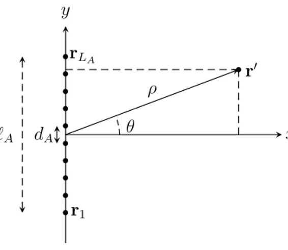
Figure 1.4: Uniform Line Array (ULA).
and its gradient
∇ψ(r, ω) = k (1.39)
An immediate interpretation of the results above is that a plane wave is a solution to the Eikonal equation (1.36) as long as the wavenumber vector k satisfies the dispersion relation (1.10). Moreover, the trajectory of acoustic rays is determined by the gradient of ψ(r, ω) as described by (1.39).
1.3.2
Spatial Filtering: the Beamformer
The methodologies for analysis and synthesis described in the subsequent chapters rely on spatial filtering. This is a signal processing technique that make use of arrays of sensors or transducers for directional signal detection [13]; originally developed in the electro-magnetic applications such as radar, sonar and radio communications, recently it has been transposed also to acoustics.
The key concept of array processing is the redundancy exploited by combining the signals of multiple sensors. In this sense, lots of methods are present in the literature ranging a large set of different applications, such as estimation of the energy distribution [14], source position esti-mation, source extraction and many others.
These vector signals are processed with the so called beamformers, which are spatial filters that applied to the spatial samples of data, en-abling the extraction of directional information about the overall acoustic energy.
In the following we consider only arrays of microphones, which are very well studied in the literature; loudspeaker arrays can be considered as the other side of the problem formulation.
Suppose we have L omnidirectional microphones and denote with
sn(t) the signal emitted by the n-th source at time t and with xl(t) the
as
xl(t) = fl,n(t)∗ sn(t) + el(t) (1.40)
where fl,n(t) denotes a generic transfer function from the source n to the
sensor l, ∗ denotes the convolution and el(t) is an additive noise, which
can be either the electronic noise of the circuits or the background noise of the environment. The Fourier transform of the model above is
Xl(ω) = Fl,n(ω)Sn(ω) + El(ω). (1.41)
By introducing the so called array transfer vector
fn(ω) = [F1,n(ω), . . . , FL,n(ω)]T (1.42)
we can write the output signal vector as
x(ω) = fn(ω)Sn(ω) + e(ω) (1.43) where x(ω) = [X1(ω), . . . , XL(ω)] T and e(ω) = [E1(ω), . . . , EL(ω)] T de-notes the additive noise vector. Finally, assuming to have N sources we can extend the previous formula exploiting the superpositon principle, obtaining
x(ω) = F(ω)s(ω) + e(ω) (1.44)
where F(ω) = [f1(ω), . . . , fL(ω)]T and s(ω) = [S1(ω), . . . , SN(ω)]T.
1.3.2.1 Far Field sources
The expression of the transfer function from the n-th source to the l-th microphone depends on the distance of the sources from the array. If sources are sufficiently far, the wavefronts can be reasonably modelled as plane waves. For linear arrays, to be considered in far field the sources should respect the following
ρ > 2ℓ
λ (1.45)
where ℓ denotes the length of the array.
In this context, the transfer function assumes the form of
Fl,n(ω) = e−j⟨kn,rl⟩ (1.46)
where, limited to a 2D scenario, kn = ωc[cos θn, sin θn]T is the wavenumber
vector of the n-th source and rl = [xl, yl]T is the position of the l-th
microphone, thus θn denotes the DoA of the n-th source.
Although many other geometries are present in the literature, this work of thesis considers only the uniform linear array, i.e. L microphones uniformly spaced at distance d along the y axis and centered in the origin as depicted in figure 1.4.
Under these assumptions, the acoustic transfer function becomes:
Fl,n(ω) = e−j ω
fn(ω) =
[
e−jωcy1sin θn, . . . , e−j ω
cyLsin θn]T (1.48)
and, exploting the so called central sensor as reference without loss of generality fn(ω) = [ ejωcsin(θn)d( L−1 2 ), . . . , 1, . . . , e−j ω csin(θn)d( L−1 2 ) ]T (1.49) Spatial aliasing condition Similarly to the temporal Shannon sam-pling theorem, a spatial aliasing condition is derived by defining a spatial
frequency
ωs= ω d sin θ
c (1.50)
and rewriting the array transfer vector (1.49) as fn(ω) =
[
ejωs(L−12 ), . . . , 1, . . . , e−jωs(L−12 )
]T
. (1.51)
We have to constrain the spatial frequency in order to avoid spatial alias-ing: |ωs| ≤ π → |ω d sin θ c | ≤ π → ω d| sin θ| c ≤ π (1.52)
that in the worst case becomes
ωd
c ≤ π → 2π d
λ ≤ π (1.53)
yielding the final condition:
d≤ λ
2 ∀θ (1.54)
Finally, if the condition (1.45) does not hold and the plane waves assumption is no longer valid, the transfer function Fl,n(ω) can be written
similarly to the Green function in (1.13):
Fl,n(ω) =
e−jωc∥rl−r′n∥
4π∥rl− r′n∥
(1.55)
1.3.2.2 Delay-and-sum beamformer (DAS)
In this section we present a simple but powerful beamformer design pro-cedure known in the literature as delay-and-sum (DAS).
Let us consider a uniform linear microphone array deployed along the y axis and centered in the origin and a source in far-field placed in r′ = ρs[cos θs, sin θs]T that emits a signal s(t). Assuming the model of
equation (1.43), our purpose is to extract the signal by applying a FIR filter to the output of the array signal:
ˆ
where hH(ω) = [h1(ω), . . . , hL(ω)]H is the vector of filter coefficients. Let
us define the variance of the output as:
E{|y(ω)|2}= hH(ω)Φxx(ω)h(ω) (1.57)
where Φxx(ω) = E
{
x(ω)xH(ω)} is the auto-covariance matrix of the
array signal.
Therefore, we can set up a minimization problem as follows: arg min
h(ω)
hH(ω)A(ω)h(ω) subject to hH(ω)B(ω) = c(ω)
where A(ω)∈ CL×L,B(ω) ∈ CL×qand c(ω)∈ C1×qare generic
frequency-dependent complex-valued matrices and q is the number of constraints. Omitting the frequency dependence, the generic solution of this opti-mization problem is given by
ho = A−1B
(
BHA−1B)−1cH. (1.58) In the specific case of the DAS beamformer, assuming the signal x(ω) to be spatially white implies that A(ω) = Φxx(ω) = I. Moreover,
con-straining the beamformer to pass undistorted the source signal is ex-ploited by using one single constraint defined as
hH(ω)f(ω) = 1, (1.59)
where f (ω) collects the acoustic transfer function from the source to each array element.
Finally, the DAS optimization problem takes the form arg min
h(ω)
hH(ω)h(ω) subject to hH(ω)f(ω) = 1, yielding to the solution
ho(ω) =
f(ω)
∥f(ω)∥2. (1.60)
As a simple interpretation, the DAS beamformer applies a delay to each microphone making sure that the desired signal is summed construc-tively. Finally, the DAS beamformer is completely data-independent, thus it requires a small effort from a computational stand point.
1.4
Plenacoustic Imaging
In this section we introduce the reader to the realm of Plenacoustic imag-ing, or soundfield imagimag-ing, as a method for acoustic scene analysis origi-nally presented in [3]. Its main advantages are that the images are gener-ated by a common processing layer and can be processed using methods inherited from pattern analysis literature.
The name is inherited from the concept of plenacoustic function (PAF) , that describes the acoustic radiance in every direction through every point in space [15]. In a 2D geometric domain, it can be written as a five-dimensional function f (x, y, θ, ω, t) of position (x, y), direction θ, frequency ω and time t.
In [2], the soundfield p(r, ω) is expressed as the superposition of plane waves with wave number vector k(θ):
p(r, ω) = 1
2π ∫ 2π
0
ej⟨k(θ),r⟩P (k(θ)) dθ,˜ (1.61)
where ˜P (k(θ)) is known as Herglotz density function and it modulates
in amplitude and phase each plane wave component. The plenacoustic function is defined as the integrand of (1.61)
f (x, y, θ, ω)≜ ej⟨k(θ),r⟩P (k(θ)) ,˜ (1.62) where the time dependencies have been omitted since we are particularly interested in the dependence on the position, direction and frequency.
In [3] the authors captures the PAF by means of microphone arrays that act as Observation Windows (OWs) for the acoustic scene. This approach consists of dividing the microphone array into subarrays, and applying the the plane-wave analysis on individual subarrays. Each di-rectional component is obtained through beamforming techniques that allows to scan the acoustic field for a discrete set of directions. In other words, the emerging image represents an estimate of the acoustic energy carried by directional components measured at several points on the ar-ray.
The subdivision into sub-arrays implies an important consideration: for the far-field assumption to be valid, sources no longer need to be in the far field with respect to the length of the global array, but only with respect to the size of the sub-arrays. On the other hand, performances degrate at low-frequencies and when the distance becomes comparable to the length of the sub-arrays.
1.4.1
The Reduced Euclidean Ray Space
In [2] a novel parametric parametrization of the ray space has been in-troduced as the domain of the plenacoustic function, in which each value associated to a ray is represented as a point in this space.
Under the radiance invariance law assumption, we can establish an equivalence between rays and oriented lines. In the 2D scenario:
l1x + l2y + l3 = 0, (1.63)
or, in vector notation,
Figure 1.5: Ray Space representation of a point source in r′.
From the latter we can state that all the vectors of the form l = k[l1, l2, l3]T,
k ̸= 0 represent the same line and form a class of equivalence. Thus, the
vector l can represent all rays with arbitrary direction.
Hence, we can think of a domain with coordinates l1, l2, l3 where the
vector l, corresponding to a ray, is a point. This domain will be referred as Projective Ray Space P. Moreover, in order to distinguish between two oppositely oriented rays lying on the same line, we can constrain k to either positive or negative values only, defining the oriented projective space.
A particular reduced ray space, called the Euclidean ray space (m, q), is derived from the projective ray space by setting
m =−l1 l2 q =−l3 l2 . (1.65)
In [3] the authors provide a detailed study of how the acoustic prim-itives can be represented in this reduced space. As we can see from equation (1.65), rays parallel to the y axis can not be represented in a limited domain; deploying only one observation window along the y axis overcomes this limitation. Moreover, since we loose the orientation of the rays, we conventionally assume the orientation toward the y axis from the positive half-plane x > 0.
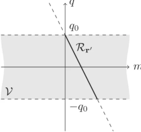
Figure 1.5 shows how a point source looks like in this reduced ray space for an OW deployed along the y axis from −q0 to +q0. The image
of a point source becomes a line in (m, q) whose parameters are the coordinates of the point. The visibility V of the array appears as a stripe between the limits−q0 and +q0 of the OW:
V = {(m, q) ∈ R × R : −q0 ≤ q ≤ q0} . (1.66)
The Euclidean parametrization introduced in [3] has been used in [4] to devise an important tool called Ray Space Transform that performs a
transformation of the signals captured by a microphone array based on a short space-time Fourier transform using discrete Gabor frames. The Ray Space Transform will be analysed in detail in the following chapter.
1.5
Conclusive Remarks
In this chapter we introduce the main issues in modelling the sound field and propagation phenomena.
First we have addressed the so called nonparametric representation, in which the acoustic field is described as a function of space and time and it is decomposed using different basis functions, foremost the planes wave decomposition. Then we have reviewed the principal methodolo-gies for soundfield reproduction, starting from the simplest two-channel stereophony up to the more immersive techniques such as Ambisonics, which is based on a spherical harmonics decomposition of the wave field, and Wave Field Synthesis, which can be described as as a sampling-interpolation process of the continuous driving function that emerges from the Kirchhoff-Helmholtz integral. These techniques are strongly motivated in multimedia applications such as gaming or telepresence; in-deed, the immersivity of a sound experience relies on the capability of rendering realistic sources and propagations. However, in addition to their peculiar limitations, these nonparametric methods result in a lim-ited sweet spot, requiring the listener to be in a specific position, e.g. inside a circular array for Ambisonics.
In the second part we have presented the plenacoustic techniques that are emerging in the last decade. The acoustic field is modelled as the superpositions of acoustic rays, propagating without angular spread. By means of uniform linear arrays of sensors and transducers, the core processing of these techniques is the beamformer, a spatial filter that scans the sound field in a given set of directions. The output is a image that can be processed with algorithms inherited from pattern analysis literature.
2
Theoretical Background
This chapter introduces the readers to the linear operator known as Ray
Space Transform, which is the most important tool this work of thesis
relies on for the analysis of sound scenes, and the concept of radiation
pattern as the angular-frenquency dependence of any acoustic object.
We start describing how a sound scene can be acquired by means of microphone arrays and analysed in a plenacoustic fashion. In plenacous-tic imaging, acousplenacous-tic primitives such as sources, observation windows and reflectors appear as linear patterns in the resulting images, thus enabling the use of pattern analysis techniques to solve acoustic problems. Briefly, the plenacoustic function (1.62) is estimated by subdividing the micro-phone array into smaller overlapped sub-arrays and by estimating each directional component for each sub-array through beamforming. The main limitation of this methodology is that performance degradates at lower frequencies and when the distance of the source becomes compa-rable to the size of the sub-array. In order to overcome this limitation, the authors of [4] propose a new invertible transformation in order to map the extracted directional information onto the reduced Euclidean ray space described in 1.4.1. This new linear operator, which takes the name of Ray Space Transform, shows perfect reconstruction capabilities and therefore is a good candidate for sound scene processing paradigms. The second section describes in detail the radiation pattern as an amplitude function of both the temporal frequency and the angles with respect to a reference direction. Inherited from the literature on anten-nas and electro-magnetic devices, the problem of modelling the radiation pattern has been investigated by many authors. In the audio equipment industry, the polar data are acquired by rotating the loudspeaker or the microphone on a turntable and measuring its output at each turntable
position [16]. The most common representation, because of its physical interpretation, is the Spherical Harmonics Decomposition, and its 2D for-mulation known as Circular Harmonics Decomposition (CHD). In both the electro-magnetic and acoustic fields, the radiation pattern is strongly related to the physical characteristics of the source, such as the dimen-sions and the materials. Thus it includes information not only about the position and orientation of the source, but, in a way, it can give a flavour of the characteristic of a object in the scene.
2.1
Ray Space Transform
In [4] the sound field decomposition relies on a new overcomplete basis of wave functions of local validity. In other words, a local space-time Fourier analysis is performed by computing the similarity between the array data and shifted and modulated copies of a prototype spatial window.
In the time domain, the local Fourier transform of a signal s(t) is defined as the discrete Gabor expansion [17]
[G]i,w = ∫ R s(t)ψi,w∗ (t)dt. (2.1) where ψ∗i,w(t) = ψ(t− iT )e−j2πWw(t−iT ). (2.2)
ψ(t) is the analysis window, i∈ Z is the time frame index, w = 0, . . . , W −
1 is the frequency band index, W is the number of frequency bins and T is the window hop size.
From G is possible to reconstruct the time signal s(t) using the local inverse Fourier transform defined as
s(t) =∑ i W∑−1 w=0 [G]i,wψ˜i,w(t), (2.3) where ˜ψi,w(t) = ˜ψ(t− iT )e−j 2π
Ww(t−iT ) and ˜ψ(t) being the synthesis
win-dow; to achieve perfect reconstruction, the completeness condition ∑
i
ψ(t− iT ) ˜ψ(t− iT ) = 1
W (2.4)
must be satisfied. The analysis and synthesis windows ψ and ˜ψ form a
pair of dual discrete Gabor frames [18].
The above Gabor frame definitions can be extended to the ray space domain. First, let us consider a continuous observation window along the y axis limited from −q0 and q0, as done in section 1.4.1, and exploit
the plane-wave expansion to model the sound field. We recall the reader that, given the wavenumber k = [cos θ, sin θ]T, the pressure field is:
The expression above can be reduced to the observation window along the y axis:
p(r, ω) = e−jωcy sin θ. (2.6)
.
Starting from the classical parametrization of the plenacoustic func-tion f (x, y, θ) (1.62), a new mapping is defined by
x = 0 θ = arctan(m) − π/2 < θ < π/2 q = y. (2.7)
Note that the first condition is derived by placing the OW along the y axis. The phase shift at position y due to a directional contribution from
θ is given by
y sin θ = y sin(arctan m) = √ ym
m2+ 1, (2.8)
where the second equality follows from known interrelations among trigono-metric functions [19].
We adopt an uniform grid for sampling the (m, q) plane and denote by ¯q and ¯m the sampling intervals on the q and m axes, respectively. In
particular, we choose qi = ¯q ( iI− 1 2 ) , i = 0, . . . , I − 1 mw = ¯m ( wW − 1 2 ) , w = 0, . . . , W − 1 (2.9)
I and W being the number of samples on q and m axes, respectively, and
we adopt the Gaussian window
ψ(y) = e−πy2/σ2 (2.10)
where the scalar σ controls the width of the window. Thus, we can write the Ray Space Transform (RST) of the acoustic field P (y, ω) in the continuous setting as follows
[Y]i,w(ω) = ∫ q0 −q0 P (y, ω)e −jω c ymw √ m2w +1ψ∗ i,w(y)dy. (2.11)
The Inverse Ray Space Transform (IRST) is defined in the same way as (2.3) in the time domain, yielding
P(Y)(y, ω) = I−1 ∑ i=0 W∑−1 w=0
[Y]i,w(ω)e
jωc√ymw
m2w +1 ˜
ψi,w∗ (y), (2.12)
-4 -3 -2 -1 0 1 2 3 4 m -1 -0.5 0 0.5 1 q 0.02 0.04 0.06 0.08 0.1 0.12 0.14 0.16
Figure 2.1: (m, q) line (in red) and magnitude of the RST for an isotropic point source, emitting a pure tone at 2 kHz, placed in r′ = [1, 0] m.
In real scenario we do not have a continuous aperture but we sample the spatial signal in a finite number of points in the space. For this purpose, let us consider a uniform linear array of L microphones displaced along the y axis between −q0 and q0 and centered in the origin, thus the
l-th microphone is placed in yl = d ( l− L− 1 2 ) , l = 0, . . . , L− 1 (2.13) where d is the distance between adjacent microphones. After discretizing (2.11) with respect to y we obtain
[Y]i,w(ω) = d L−1 ∑ l=0 P (yl, ω)e −jk√ylmw m2w +1e−π(yl−qi) 2 σ2 . (2.14)
The discrete ray space transform can be conveniently written in matrix form by introducing the matrix Ψ(ω) ∈ CIW×L whose element in row l
and column (i + wI + 1) is [Ψ]l,i+wI+1= e −jk√ylmw m2w +1 e−π(yl−qi) 2 σ2 d. (2.15)
We also introduce the canonical dual matrix ˜Ψ∈ CIW×L corresponding to the pseudo-inverse of Ψ
˜
which, among all the infinite matrices that could play the role of dual matrices of Ψ (due to the overcompleteness condition IW ≥ L), is the one that guarantees the coefficients to have minimum norm.
Finally we introduce also the vector y∈ CIW×1 obtained by rearranging
the elements of Y as
[y]i+wI+1 = [Y]i,w. (2.17)
Therefore, we can write the discrete ray space transform as
y = ΨHp (2.18)
and its inverse
p(Y)= ˜ΨHy. (2.19)
In order to give the reader a graphical interpretation, figure 2.1shows the linear pattern and the magnitude of the discrete ray space coefficients of the acoustic field of a point source in r′ = [1, 0] meters, emitting a tone at 1kHz. For the sake of completeness, the parameters of the RST are
σ = 22.5cm, L = 32 microphones with d = 7.5cm (q0 = 1.1625m),
¯
q = d/2 = 3.75cm and ¯m = 4.47cm.
2.1.1
Remarks
Notice that the array has, inevitably, a limited extension, bounded within
−q0 and q0. Therefore, in addition the the moving spatial window (2.10),
there is a fixed rectangular window of length 2q0.
The interpretation of (2.11) is immediate upon considering a single spatial window, i.e. upon fixing i. The expression is intepreted as the beamforming operation applied to the aperture data that have previously been weighed by a Gaussian spatial windowing function centered at qi.
Thus, [Y]i,:collects the outputs of multiple beamforming operations, each computed from a specifically weighed portion of the aperture data.
2.1.2
Source Localization in the Ray Space
In this section we discuss one example of application, where the analysis and processing of the acoustic signal are done in the ray space presented above. The example is taken from [4], where the author aims at localizing acoustic sources in near field condition.
Localization is based on a wide band extension of the ray space coeffi-cients. Denoting with |Y(ωk)| the magnitude of the ray space coefficients
at frequency ωk, the wideband magnitude estimated is defined as
Y = K/2∏ k=0 E{|Y(ωk)|} 2/K , Y ∈ RI×W, (2.20)
where K/2 is the number of considered frequencies. In the simulations the expectation is approximated by an average over J = 10 time frames:
E{Y(ωk)} = 1 J J−1 ∑ j=0 Y(j)(ωk), (2.21)
where Y(j)(ωk) = ΨH(ωk)u(j)(ωk) are the ray space coefficients
comput-edt at the j-th time frame from the array signal u. As stated in section
1.4.1the image of a point source in the reduced ray space (m, q) is a line whose parameters are the (x, y) coordinates of the point source. There-fore, localization is accomplished by estimating the peaks for each row
Yi,:. The position of the source is estimated through a least-squares
re-gression of the locations of the peaks. In particular, the founded peaks at value ˆmi are collected in the vector ˆm = [ ˆm0, . . . , ˆmI−1]T; then we
introduce a matrix ˆM = [− ˆm, 1] and the vector q = [q0, . . . , qI−1]T that
collects the position of the centres of the spatial windows on the y axis. Finally, since ˆMr′ = q the position r′ is estimated as
ˆ r′ = ( ˆ MTMˆ ) ˆ MTq. (2.22)
2.2
Radiation Pattern
This section introduces the concept of radiation pattern as a angular-frequency dependence of the amplitude of a signal emitted/received by a source/microphone. In general, acoustic sources present emission pat-terns which are far from being omnidirectional, i.e. constant with respect to the directions, in particular at higher frequencies [20]. Considering a loudspeaker, for example, the complexity of its radiation pattern at a given frequency depends on the ratio between the size of the source and the considered wavelength [21]. As a matter of facts, the radiation pat-tern influences the way the acoustic waves propagate within a sound scene [22], [20], with direct implications on the behavior of the most audio processing algorithms.
Many authors in the literature assume the radiation pattern to be constant over both the frequency and the directions of propagation, thus either simplifying the algorithms and the results or introducing an equal-ization stage, e.g. [23]. Later, some authors have assumed arbitrary radiation directivities in their soundfield rendering algorithms (e.g. in Ambisonics [24] and in Wave Field Synthesis [25], [26]).
The rest of this chapter is organized as follows. First we give some formal definitions of radiation pattern, along with the necessary assump-tions for the correcteness with respect to the acoustic propagation laws. Then we present a parametric approach to model the radiation pattern in a efficient way, inherited from the literature on antennas and EM prop-agation. This method decomposes the radiation function as a sum of cosines of multiples of the directions, the so-called circular harmonics.


![Figure 1.3: The Huygens principle (courtesy of [1]).](https://thumb-eu.123doks.com/thumbv2/123dokorg/7500867.104484/22.892.289.599.165.392/figure-the-huygens-principle-courtesy-of.webp)